Effect of climate shocks on rural household welfare dynamics in Ethiopia: evidence from panel data

Abstract

Climate shocks have been shown to reduce agricultural output and cause production fluctuations in developing countries. When livelihoods depend on rain-fed agriculture, like in Ethiopia, climate shocks will translate into consumption shocks. Despite significant improvements in household consumption in Ethiopia, shocks caused by climate and other factors are negatively affecting household consumption dynamics. Therefore, examining household consumption dynamics in the context of climate-induced shocks helps to guide resilience capacity and establish appropriate programs and interventions. The study used a three-round panel dataset based on the Ethiopian socioeconomic survey and spatial rainfall data. The results of the linear dynamic panel model show that lagged consumption values, market shocks, and changes in rainfall positively affect consumption dynamics. In contrast, production, temperature, and rainfall shocks have an inverse relationship. Strategies for mitigating climate shocks and consumption aftershocks help stabilize consumption over time. Support to strengthen household coping strategies may involve restoring existing livelihoods and forms of production or reducing household vulnerability. Therefore, government intervention is required for asset accumulation programs to support household coping strategies and responses to shocks. In addition, the dynamic link between consumption and essential socioeconomic and institutional factors must be considered to minimize the impact of climate shocks on consumption dynamics.

Keywords:

• climate shocks
• consumption dynamics
• linear panel dynamic model
• Ethiopia
• household

REVIEWING EDITOR:

• M. Luisa Escudero-Gilete, Senior Editor, Universidad de Sevilla, Spain

SUBJECTS:

• Social Sciences
• Development Studies
• Development Studies
• Development Policy
• Economics and Development
• Environment & the Developing World
• Sustainable Development
• Economics, Finance, Business & Industry
• Environmental Economics
• Economics

1. Introduction

In sub-Saharan Africa, climate shocks have an adverse impact on household welfare and are more severe than in developed countries (Boyd et al., 2013; Pironon et al., 2019). Ethiopia is subject to high climate variability and extreme hazards that negatively affect the agricultural sector (Conway et al., 2019; Kamali et al., 2018; Sietz et al., 2017) since rainfed agriculture with limited use of modern agricultural management practices makes it more vulnerable (Shukla et al., 2021). Projected changes in climate show increased frequency and severity of droughts, floods, hot days and nights, and erratic rainfall (Liou & Mulualem, 2019; Nikulin et al., 2018). Ethiopia’s agriculture and economy are vulnerable to observed climate changes (Yalew et al., 2018). Therefore, strengthening the capacity of households to cope with climate change and variability is important in Ethiopia, as agriculture contributes to the backbone of most of the Ethiopian economy.

Smallholder farmers¹ are more vulnerable to climate shocks (Shiferaw et al., 2014) for the following reasons: First, the livelihoods of households are highly dependent on agriculture, and the sector is susceptible to the weather (Dube & Sivakumar, 2015) and is constrained by different socioeconomic and biophysical factors (Asfaw et al., 2011; Abebe and Sewnet, 2014). Second, the adaptive capacity and ability to adopt climate-smart agricultural practices, and resilient capacity of households are low (Gebrelibanos & Wondimagegn, 2018; Lohmann & Lechtenfeld, 2015; Narloch & Bangalore, 2018; Shehu & Sidique, 2014). Finally, developing countries like Ethiopia have weak and fragile institutional setups that lack early warning systems for extreme events. As a result, extreme weather events affect household well-being.

Furthermore, previous studies have identified at the country level (Hallegatte et al., 2016, 2018), failing to capture the micro-level impact. Furthermore, the state of academic discourse also continues to produce controversial findings on the effects of climate shocks on household-level consumption dynamics (Akerele & Adewuyi, 2011; Edoumiekumo et al., 2013; Gounder, 2013; Lekobane & Seleka, 2017; Mduduzi & Talent, 2018; Sekhampu, 2013). For example, Nordhaus (2014), Hsiang et al. (2017) and Letta et al. (2018) find that the effects of climate shocks are heterogeneous across locations. Equally important is that household absorptive capacity, capital sources and livelihood strategies heterogeneously determine climate shocks. To the knowledge of the researchers in Ethiopia, Gao and Mills (2018) examine the impact of precipitation on consumption using macro panel data. However, this paper only considers rainfall as an indirect indicator of the shock of climate change and does not indicate the impact at the micro level. In addition, previous empirical studies have been undertaken in Ethiopia by Akerele and Adewuyi (2011), Porter (2012), Gounder (2013), Lindquist and Lindquist (2012), Brück and Kebede (2013), Edoumiekumo et al. (2013), Seff and Jolliffe (2016), Lekobane and Seleka (2017) Hirons et al. (2018), Niles and Salerno (2018), and Araya et al. (2019) focus on location-specific, specific factors, and snapshot data that only partially reflect the cause.

Therefore, the existence of knowledge gaps and the effects of existing climate shocks have always attracted the interest of policymakers. Overall, the shortcomings of previous studies include (i) empirically, few studies investigating the impact of climate-related shocks on household consumption at the national level. and (ii) the methodological and statistical inferences of most studies are cross-sectional based, (iii) most climate-related variables reported by rural households may be biased in reporting. We, therefore, examine the effects of climate-related variables and other factors on household consumption dynamics in Ethiopia to contribute to and enhance the existing knowledge gap.

2. Conceptual framework

Specific and covariate shocks affect household welfare by negatively impacting various household resources. In particular, the effects will be more severe on welfare unless households can ensure appropriate coping strategies and interventions (Dell et al., 2014; Skoufias & Vinha, 2013). The Common Sustainable Livelihoods Framework suggests that human, social, physical, financial, and natural capital are essential for better household well-being under shocks. When households face specific climate-induced shocks, different household assets will mitigate the shock’s negative impact on household welfare.

Climate shocks directly or indirectly affect resource availability and/or availability. For example, climate and change shocks directly affect livestock and crop production so that households can reduce consumption with less resilience. Similarly, productivity will decrease if a household finds it difficult to obtain financial capital to purchase agricultural inputs. The following conceptual framework is developed based on the key concepts and fundamental theories (Figure 1). The basic idea is that the impact of climate-induced shocks may not be directly observable because the number of shocks depends on the resilience of the household aftershocks.

Figure 1. Conceptual framework.

Source: Adopted from Sustainable Livelihood Framework (SLS), Gao and Mills (2018) work based on empirical literature review.

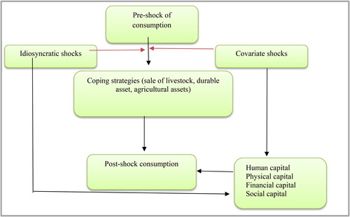
The impact of climate shocks on consumption depends on the resources and resilience of households (Skoufias & Vinha, 2013). Extreme shocks sharply reduce agricultural output, resource allocation among farmers, and optimal consumption pathways. Households cannot protect agricultural production when extreme events and rainfall fall below the minimum threshold (Porter, 2012; Skoufias & Vinha, 2013). Finally, the net impact of climate shocks on consumption depends on the resilience of households (Auffhammer & Schlenker, 2014) and indirectly on the effects of market shocks on consumption through food prices (Fischer et al., 2002).

3. Materials and methods

3.1. Data and variables

The study used Ethiopian Socioeconomic Survey (ESS) data and Climate Hazards Group Infra-Red Precipitation with Station (CHIRPS) rainfall data to examine how rainfall affects households. The ESS was collected three times (2011–2012, 2013–2014, and 2015–2016) and included household demographics and socioeconomic conditions. Additionally, rainfall data from CHIRPS was downscaled to enumeration areas (EAs) to create a historical rainfall dataset at the household level. If there was a shortage of rainfall (defined as a deviation from the historical mean rain), that was coded as a binary variable (Michler et al., 2019; Ward & Shively, 2015).

The ESS study collected information from rural and small-town areas in Ethiopia. The ESS sampled households in nine regions, including Amhara, Oromia, SNNP, Tigray, Afar, Benshangul Gumuz, Gambella, Harari, and Somali regional states of Ethiopia and Dire Dawa city administration. The ESS used two-stage probability sampling techniques to select EAs. The first sampling stage involved selecting EAs and sample households from the Agricultural Sample Survey (AgSS) in the second stage. The AgSS EAs were selected based on a probability proportional to the size of the regional population. For the rural sample, 290 EAs and 43 EAs from small towns and 12 sample households were selected for each EA. The second and third waves added 100 urban EAs, including Addis Ababa. In each urban EA, 15 sample households were selected. Adding urban EAs increased the sample size from 433 to 439 EAs. The final interviewed sample household was 3969 in the first wave, 3776 in the second wave, and 5466 in the third wave. However, maintaining the balanced panel sample for this analysis restricted the final analysis to households not considered in the three rounds, outliers, and missing information. Finally, this study evaluated a balanced sample of 3220 households in each round with the corresponding sample weight for the poststratification adjustments to ensure that all regions were represented.

Consumption expenditure in an adult equivalence unit better captures households’ consumption smoothing behavior and is thus preferred as a better indicator of household welfare in developing countries like Ethiopia (Haughton & Khandker, 2009). All expenditures are expressed in 2016 and reflect real annual consumption expenditures per adult equivalent. According to Porter (2012) and Dercon et al. (2012), food expenditure, education, and nonfood (durable noninvestment, nonfood items, and health) are the main components of aggregate consumption. The spatial deflators provided by Ministry of Finance and Economic Development (MoFED) (2014) and consumer price index deflators provided by the World Bank (2015) were used to adjust price differences over time.

3.2. Econometric model

Fixed and random effects estimation techniques are widely used for continuous outcome variables in panel data. Fixed effects solve the problem of standard selection and yield unbiased coefficient estimates. For example, Solomon and Giuseppe (2018) examined the impact of weather shocks on food expenditure using a fixed-effects model assuming unobserved heterogeneity across units. In addition, Mduduzi and Talent (2018) also used a fixed effects regression model to estimate the variables of welfare dynamics. Fixed effects lead to bias in parameter estimates in short-panel data. According to Roodman (2009), linear dynamic GMM estimators are designed for a "small time, large sample" that can contain fixed effects and separate from idiosyncratic errors correlated within households and cause heteroscedasticity.

In this case, the random effect overcomes this problem and adds the mean values of the time-varying variables to loosen the assumption that there is no correlation between the unobserved characteristics and the variables simultaneously (Mundlak, 1978). In addition to the fixed effect and random effect models, if variance and autocorrelation problems exist in the micropanel data for consumption analysis, a linear dynamic panel model can apply using Arellano-Bond, including the lagged value as an instrumental variable. However, the estimator is inefficient because the instrumental variable does not exploit the condition of all available times. In addition, Blundell and Bond (1998) also claim that the tool used in the first difference GMM becomes less informative because the autoregressive parameters increase in the direction of unity and the variance of the unit-specific effects.

Arellano and Bover (1995) and Roodman (2009) proposed the orthogonal deviation transform to eliminate fixed effects by subtracting the mean of all available future observations and multiplying with the scale factor. Since the lagged consumption observations do not enter the transformation formula, they are still orthogonal to the converted errors and are available as tools. In fact-finding of micro panel data, lagged values are sometimes a poor instrument for the first differenced covariates, leading to an inefficient estimator. Spending on current consumption can depend on consumption in previous periods and lead to an endogenous problem. In addition, there are concerns about a potential causal relationship between coping strategies and consumption. A household may use a coping strategy in the face of a shock because household consumption falls, and the latent endogeneity of coping strategy variables must be controlled during the estimation process. In this case, a dynamic panel data model would be more suitable for estimation. Blundell and Bond (1998) reported that subtracting the past value from the present value leads to information loss. Therefore, the system’s GMM estimator helps to retrieve information with orthogonal deviations. The Arellano-Bond and Blundell-Bond GMM linear estimators have one-step and two-step variants. However, the two steps are asymptotically more efficient, and the standard errors reported tend to be biased downward (Arellano & Bond, 1991; Blundell & Bond, 1998). In addition, Windmeijer (2005) argued for the importance of two-step compensation for reduced bias and that a finite sample correction could be derived. Therefore, the two-step robust estimate is more efficient than the one-step strong estimate in the GMM system.

Accordingly, a linear dynamic panel model was used to examine the impact of climate shocks on household consumption dynamics. The model includes demographic, socioeconomic, and institutional factors, climate shocks, and lagged consumption. Therefore, the model is (1) $${\text{lnC}}_{\text{it}}={\text{β}}_{0\hspace{0.17em}}+{\text{αlnC}}_{\text{it}-1}+{\text{X}}_{\text{it}}{\text{β}}_1+{\text{Cl}}_{\text{t\hspace{0.17em}}}^T{\text{β}}_{2\hspace{0.17em}}+{\text{μ}}_{\text{i\hspace{0.17em}}}+{\in }_{\text{it\hspace{0.17em}}}$$(1) where

• ${\mathrm{\text{lnC}}}_{\mathrm{\text{it}}}$ = consumption of household i in year t.

• α = autoregressive coefficient parameter.

• $\mathit{\text{ln}}{\mathrm{C}}_{\mathrm{\text{it}}-1}$ = consumption expenditure of household i at time t.

• ${\mathrm{X}}_{\mathrm{\text{it}}}=$ a vector of time-variant and invariant household characteristics.

• ${\mathrm{\text{Cl}}}_{\text{t}}^{\mathrm{T}}=$ a vector of climate-induced shocks on households in year t.

• ${\mu }_{\text{i\hspace{0.17em}}}$= fixed effects.

• ${\epsilon }_{\text{it\hspace{0.17em}}}$ = idiosyncratic error term

The estimation considers household errors and within-panel correlation. Coping strategies of households in Eq. (1)(1) $${\text{lnC}}_{\text{it}}={\text{β}}_{0\hspace{0.17em}}+{\text{αlnC}}_{\text{it}-1}+{\text{X}}_{\text{it}}{\text{β}}_1+{\text{Cl}}_{\text{t\hspace{0.17em}}}^T{\text{β}}_{2\hspace{0.17em}}+{\text{μ}}_{\text{i\hspace{0.17em}}}+{\in }_{\text{it\hspace{0.17em}}}$$(1) instrumented lagged consumption of households since α measures the shocks’ net impact on consumption after moderating adverse effects.

4. Results and discussion

Climate-induced shocks and variables are implemented at the household level. The percentages and mean values of trends in climate-related shocks from 2012 to 2016 are summarized in Table A1. The results show that the proportion of households reporting drought, production and market over time is 18%, 22%, and 20%, respectively. Approximately 15% of those in Wave I, 9% in Wave II, and 31% in Wave III of households perceive and report the existence of drought shocks. The proportion of self-reported drought shocks decreased significantly between 2012 and 2014 and increased between 2014 and 2016. Similar patterns for production and market shocks have been observed due to climate change and variability but to quite different degrees. The average daily temperature in 2012 was 19.36 °C. In 2014, it was 19.4 °C; in 2016, it was 19.39 °C. The average daily temperature fluctuates slightly over time, but regions differ significantly. The average monthly rainfall in 2012–2016 was 1083.93 mm, while the average in 2012, 2014, and 2016 was 1082.42 mm, 1084.35 mm, and 1085 mm, respectively. Rainfall variability increased by about 2 mm from 2012 to 2014 and 1 mm from 2014 to 2016. The variation of rainfall in all rounds is close to 4004 mm. The significant variation in annual and seasonal rainfall negatively affects Ethiopia’s agricultural system and production.

Demographics, socioeconomic factors, and institutions influence household consumption. Most households in the sample were male-headed (73.9%). The proportion of female-headed households was lower than the national average. Most sample respondents were married (76%) and single (73%) from 2012 to 2016. From 2012 to 2016, the average household size for adults and overall was 5 and 4, respectively. This aligns with rural Ethiopia’s estimate in 2015/2016, where family size was also 5 and 4 in adult equivalent (Ministry of Finance and Economic Development (MoFED), 2014). The average age of household heads was 45, 46, and 48 in 2012, 2014, and 2016, respectively.

Table A3 shows that education, livestock, cultivated and noncultivated land, additional income, and farm asset index are vital indicators of rural household wealth. Sample households had an average education level of 6 grades from 2012 to 2016. The average livestock holding was 2.3 TLU, slightly increasing over time. Of the average landholding size (1.35 hectares), 76.4% were cultivated, while 23.6% remained noncultivated. Trends in cultivated and noncultivated land varied over time. The landholding is more significant than Ethiopia’s national average of 1.17 ha/household (Ministry of Finance and Economic Development (MoFED), 2014). Income sources such as safety net programs, remittances, and farm/nonfarm activities also impact consumption.

Table A4 shows that credit, extension, and markets affect household consumption through their impact on access to inputs, output markets, information, knowledge, technology transfer, and capacity building. The average distance to the main market was 66.4 walking minutes. Only 32% of household heads had access to extension services, which indicates that Ethiopia’s level of extension service was low. Access to extension services provides necessary information for effective resource utilization and technology availability, leading to improved consumption. Around 11% of sampled households have had credit access from 2012 to 2016, an exceptionally low percentage. By 2016, access had increased to around 16%, with a 7% rise from 2012 to 2014.

Before estimating each econometric model, appropriate tests were conducted for normality, multicollinearity, heteroskedasticity, autocorrelation, and other specification problems. Normality tests indicated that the consumption expenditure per adult equivalent was not normally distributed (P = 0.00), so it was transformed with a natural logarithm. Multicollinearity was checked with the variance inflation factor (VIF), which showed a mean value of 1.7, below the expected threshold of 2 (O’Brien, 2007). Linear correlation among independent variables was rejected. Model specification passed the Ramsey-reset test (P = 0.00, F value = 16.77). However, omitted variables were found. The Breusch-Pagan test indicated heteroskedasticity (P = 0.053). Use the robust option for a corrected variance estimate if heteroskedasticity is the issue. The fixed effects estimator is efficient when errors are not serially correlated. Diagnostic tests show a correlation between residual autocorrelation and residual lag value. Using a fixed or random-effect model to estimate the effect of climate-induced shocks on consumption dynamics did not give unbiased estimates.

Researchers utilized the linear dynamic panel model with Arellano-Bond estimation and lagged annual consumption expenditure to solve specification problems, heteroscedasticity, and autocorrelation issues. The Mata version of the model includes using forward orthogonal deviations instead of first differences. However, using lagged covariates as instruments for first-differenced regressors may be ineffective due to information loss (Blundell & Bond, 1998). The system GMM estimator improves efficiency by using two equations to obtain additional instruments that correct autocorrelation. One-step estimation reports Sargan statistic is not robust to heteroskedasticity or autocorrelation. Hansen J statistic, minimized in the two-step GMM criterion function, is robust and more efficient. J test has a problem, weakening the Sargan statistic in two-step GMM cases. Analysis instrumented with coping strategies and the previous year’s self-report drought.

Both the Sargan test and Hansen test of overidentification restrictions χ² (21) values were 5.48 (P = 0.34) with no problem of overidentification but not weekend and 52.12 (P = 0.00) robust by instruments. The linear dynamic panel model result on climate-induced shocks on household consumption expenditure in Ethiopia is reported in Table 1. Production shocks, market shocks, rainfall, and temperature significantly affect household consumption and expenditure dynamics. In Ethiopia, production shocks, mean rainfall and mean temperature negatively affect consumption expenditure, but market shocks cause a surge in consumption expenditure dynamics.

Table 1. Regression results of the linear panel dynamic model.

Variables	Two-step system GMM		One-step system GMM
	Coefficient	Corrected Std. Err	Coefficient	Robust Std. Err
Lag_consumption (log)	0.0691**	0.0346	0.4446***	0.0304
Production shock	−0.0713**	0.0344	−0.0227	0.0334
Market shock	0.0695***	0.0190	0.0738***	0.0182
Temperature	−0.0068***	0.0024	−0.0050***	0.0019
Rainfall	−0.0003***	0.0000	−0.0002***	0.0000
Monthly rainfall variability	0.0002**	0.0001	0.0001	0.0001
Sex (1 = Male)	−0.0070	0.0193	−0.0191	0.0158
Age of head	−0.0028***	0.0005	−0.0015***	0.0004
Family size	−0.0780***	0.0045	−0.0503***	0.0039
Dependency ratio	−0.0349***	0.0084	−0.0287***	0.0075
Education	0.0070***	0.0008	0.0045***	0.0007
Cultivated land	−0.0001	0.0005	0.0002	0.0004
Noncultivated land	0.0062**	0.0029	0.0048**	0.0021
Livestock holding	0.0160***	0.0028	0.0125***	0.0025
Farm income	0.0683***	0.0059	0.0458***	0.0053
Nonfarm income	0.0685***	0.0147	0.0350***	0.0135
Remittance	0.0000	0.0000	0.0000*	0.0000
PSNP income	−0.0001***	0.0000	−0.0001	0.0000
Distance to market	−0.0017***	0.0002	−0.0011***	0.0002
Extension access	−0.0226	0.0155	−0.0055	0.0138
Credit service	0.2341***	0.0212	0.1628***	0.0201
Constant	7.8131***	0.3179	4.7374***	0.2834

Number of observations 9660.

Symbols: ***, ** and * indicate significance at the 1%, 5% and 10% levels, respectively.

Source: Author’s computation based on ESS (2012, 2014, and 2016) and CHIRPS.

A lagged value of consumption expenditure had a significant and positive effect on current consumption expenditure. A 1% increment in the one-period lagged consumption expenditure would increase the consumption expenditure by 0.069% for a given household. This implies that from the dynamic panel model, different coping strategies (livestock sales, durable asset sales, farm machinery/property sales) and drought self-reports have different effects in the second equation of the two-step system GMM. Notably, during the drought and production shock, households simultaneously faced pressure to sell livestock and other assets, increasing food consumption through the market. Therefore, if climate shocks cause market shocks, the results regarding households’ ability to cope and drought perceptions and predictions will be different. This finding is against the literature, which asserts that each additional lagged consumption value has a negative and statistically significant effect on future consumption. The impact of climate shocks on consumption depends on the adaptive capacity of households, which is also confirmed by Bryan et al. (2014), Khanal et al. (2017), and Castells-Quintana et al. (2018).

Households that have experienced production and market shocks are the causes of the decrease and increase in consumer spending, respectively. Specific and covariate shocks affect agricultural output and indirectly affect agricultural product prices. Therefore, production shocks negatively affect consumption. The available literature also reveals the negative impact of shocks on agricultural production directly and thus on the welfare of people in developing countries (Cabas et al., 2010; Fisher et al., 2012). However, if households can absorb and respond to production shocks, the consumption incentive will weaken over time. In this case, the market shock affects consumption positively because nominal food expenditure will increase due to increased food prices and consumption will decrease as households are affected by floods, heavy rains, and droughts in Ethiopia.

The results of the two-step system of GMM, rainfall, and temperature estimates show a negative and significant association with consumer spending. A unit temperature of °C per day and an increase in rainfall in millimeters per month lead to a decrease in the consumption of a given household by 0.0068% and 0.0003%, respectively. The transition from lower to maximum temperature leads to a significant reduction in overall consumption and food consumption. This finding indicates that climate change will affect food-related consumption through agricultural production and prices. The effect of temperature on household consumption growth on food consumption growth is more significant than overall consumption growth, as most households are subsistence in Ethiopia (Letta et al., 2018). Poor households have a weak ability to cope with future climate-related shocks and that consumption growth may be reduced. Other evidence has reported a negative relationship between consumer spending and temperature (Solomon & Giuseppe, 2018). Heavy rainfall leads to a decrease in household consumption expenditure. This could be due to several reasons. First, better rain helps rural households have more food than no rain; therefore, food-related spending will decrease. Second, based on reasonable and adaptive expectations, heavy rainfall causes households to save more and accumulate various reserves for the future instead of consuming and spending more now. This is also revealed by Félix and Romuald (2014), changes in rainfall trends over time causes a source of uncertainty and volatility in consumption. Contrary to the above results, Kumar and Sharma (2013) find a positive effect of rainfall on agricultural production and farm income.

Annual rainfall variability positively affects consumption expenditure and is significant at a 5% level. The rainfall standard deviation is below historical levels and increases expenditure dynamics. Coromaldi (2020) found that slight rainfall variability benefits income up to a limit. Coping strategies help flatten consumption, despite rainfall variability. During a severe rainfall failure, smoothing mechanisms may not work. Rainfall insurance or drought-triggered safety nets could help. Short-term shocks affect household consumption (Seff & Jolliffe, 2016). Poor face consumption volatility due to adverse weather risk and coping mechanisms are used for ex-post shocks and adaptation strategies for ex ante shocks (Castells-Quintana et al., 2018).

Household age negatively impacted consumption dynamics (P < 0.01) in one-step and two-step system GMM. Older households may prioritize nonfood expenses, such as health over schooling as they follow the life cycle consumption theory. Additionally, larger families had a significant negative impact on consumption expenditure. Large Ethiopian families consume less and save more due to fewer job opportunities and less participation in off-farm activities. Studies by Sekhampu (2013), and Lekobane and Seleka (2017) supported the negative correlation between household size and consumption.

Contrary to the above findings and arguments, family size positively affects consumption by increasing income through the excess supply of labor force, the marketable amount, and the capability to spend for nonfood items. More household members mean higher consumption expenditure due to different food and nonfood items, as found in Ayalneh and Abebaw. The overall effect of family size depends on the two effects within the household. The dependency ratio also has a negative impact on consumption expenditure over time. Households with economically inactive members have a higher dependency ratio and consume less. An increased dependency ratio puts an extra burden on the household and decreases consumption expenditure. Mduduzi and Talent (2018) claimed that having dependent families reduces spending on healthcare and education.

Household education level positively and significantly affects consumption at a 1% significance level using two-step and one-step GMM estimation techniques. This result implies that educated household heads are better positioned for better consumer spending. This finding is realistic because educated households are more likely to participate in nonfarm income sources. Household experience is increased to manage farming activities, have better agricultural productivity, and leverage their knowledge to generate higher incomes than their less educated counterparts. This result is like Lindquist and Lindquist (2012) and Hirons et al. (2018) reporting that education positively affects consumption motivation. In addition, a household head with higher education helps to participate in the formal sector, increase household income and improve food consumption (Mduduzi & Talent, 2018).

Noncultivated land positively affects consumption dynamics at 5% significance. Its size is essential for livestock production in Ethiopia, as it enables grazing and adopting improved technologies, leading to increased income and consumption. Land plays a vital role in crop production and livestock grazing. Larger livestock-holding sizes in TLUs contribute significantly to consumption per adult equivalent at a 1% significance level. Increasing livestock by one TLU raises consumption expenditure by 0.016%. Livestock is a vital source of income for rural households, providing liquid assets for spending on food and nonfood items. As noted in previous studies, oxen are also used for draft power, plowing land, and sharecropping (Abera and Zeller, 2012; Degye, 2013; Dereje & Haymanot, 2018).

Farm and nonfarm incomes significantly and positively impacted consumption expenditure in the two-step system GMM. A percentage increase in both kinds of income led to corresponding consumption expenditure increases of 0.0693 and 0.0685 percent over time. More substantial farm and nonfarm incomes allowed households to consume better and cope with economic shocks and consumption shortfalls by selling agricultural products. This income also boosted confidence in consumption. Studies by Girma and Deginet (2012), Hirons et al. (2018), and Niles et al. (2018) show that a household head’s income from farming and non-farming sources enhances household consumption. However, PSNP income significantly negatively impacts consumption expenditure, leading households to prioritize investing in agriculture and saving over consumption. PSNP income benefits the poorest and most vulnerable households, who are more likely to spend it on food than other expenses. The long-term impact on consumption depends on household saving patterns, but research indicates a different outcome than previously suggested by Berisso (2016), and Hirons et al. (2018).

Household travel distance to the market correlates negatively with consumption expenditure. Poor market access leads to lower consumption growth. Related results were found by Barbier and Hochard (2018). Credit use is statistically significant and positively impacts consumption expenditure, playing a vital role in smoothing basic food and nonfood requirements during cash constraints and reducing consumption fluctuations due to shocks such as drought, flooding, and illness. Furthermore, credit access improves rural households’ input purchases and nonfood spending. Ethiopian households benefit from formal credit through long-term investments and enhanced well-being. Nevertheless, limited access negatively impacts consumption, adaptation, and coping during climate-induced shocks. For ex-ante shocks, households hold low-return liquid or diversified livelihood strategies (Bryan et al., 2014; Castells-Quintana et al., 2018).

5. Conclusions

Despite the substantial improvements in household consumption over time, key factors still adversely affect consumption dynamics at the household level. Access to credit, education, noncultivated land, livestock farms, and nonfarm income might help households build up assets and income; thus, it smooths consumption. In addition to demographics, socioeconomic and institutional factors, climate-induced shocks also adversely affect consumption dynamics in Ethiopia. The linear dynamic panel model results show that the lag value of consumption, market shocks, and rainfall variability positively affect consumption dynamics. In contrast, production shocks, temperature, and amount of rainfall had a negative relationship.

It enhances the purchases of agricultural inputs and productive assets, improves consumption, and protects against climate-induced shocks. Investment in human capital is more effective by giving age-based skill training and creating job opportunities for households with a larger family size and a high dependency ratio; as a result, it helps to improve household consumption dynamics. Reducing family size through family planning training also improves consumption.

Property sales help households cope with climate shocks and support consumption. Building resilience through diversification of assets, sources of income and agricultural investments improves well-being and reduces negative impacts. Support can be linked to improving the livelihoods and mobility of vulnerable households, and governments should provide social protection and climate resilience programs. Improve access to institutional services by removing obstacles to credit for households without social security. Encourage the expansion of formal credit financial institutions for market integration and credit opportunities to facilitate food consumption during climate shocks. Improve resource efficiency and agricultural diversification through land use enhancement, livestock and crop diversification, and off-farm activities.

Researchers also highlight important considerations for policymakers to note in designing policies related to the dynamic relationship between climate-induced shocks and household consumption expenditure. This helps households rapidly respond to the adverse effects of climate-related shocks. The findings seek to assist in the informed decision-making process to increase the resilience capacity of households to adverse effects of climate-induced shocks while considering demographic, socioeconomic, and institutional conditions in Ethiopia.

Acknowledgments

The authors are grateful to Haramaya University, the School of Agricultural Economics and Agribusiness, the German Academic Exchange Service (DAAD), and the African Economic Research Consortium (AERC) for generous funding support. We are also thankful to the invited reviewers for their insightful comments.

Disclosure statement

The authors reported no potential conflict of interest.

Additional information

Notes on contributors

Aemro Tazeze Terefe

Aemro Tazeze Terefe is an assistant professor and researcher in the Department of Agricultural Economics at Bahar Dar University, Ethiopia. His main area of expertise is development economics, including multidimensional poverty, food security, climate change and variability, impact evaluation, agricultural marketing, production efficiency, and technology adoption.

Mengistu Ketema Aredo

Prof. Mengistu Ketema Aredo was formerly a professor of Agricultural and Resource Economics at Haramaya University and is now the CEO of the Ethiopian Economics Association. He has a PhD in Agricultural Economics from Justus-Liebig University and extensive research experience in sustainable development, environmental economics, and policy analysis.

Abule Mehare Workagegnehu

Abule Mehare Workagegnehu was previously an assistant professor at Haramaya University and is now a director of partnerships and communication at the Ethiopian Economic Association. He has a PhD in Agricultural and Resource Economics from Lilongwe University of Agriculture and Natural Resources. Abule has research experience in Agricultural marketing, international trade, environmental and resource economics, and more.

Wondimagegn Mesfin Tesfaye

Wondimagegn Mesfin Tesfaye has a PhD in Economics from Maastricht University and currently works at the World Bank Group’s Ethiopia Country Office. His research interests include development economics, impact evaluation, mathematical programming, social networks, and various economic and development problems.

Notes

1 In the Ethiopian context, smallholder farms are those that are less than 2 hectares in size, have limited resources, and most of the labor sources for farming activities are operated by family members (Rapsomanikis, 2015). Therefore, in the context of this research, the authors use households, farmer households, and smallholder farmers interchangeably.

Appendix

Table A1. Summary statistics of climate-induced shocks related variables in the panel data.

	Climate-induced related shocks and climate variability over survey years of the panel
	2012		2014		2016		Pooled
Variables	Frequency /Mean	Percent /Std. Dev	Frequency /Mean	Percent /Std. Dev	Frequency /Mean	Percent /Std. Dev	Frequency /Mean	Percent /Std. Dev
Drought shock	(483)	(15)	(290)	(9)	(998)	(31)	(1739)	(18)
Production shock	(580)	(18)	(386)	(12)	(1127)	(35)	(2125)	(22)
Market shock	(773)	(24)	(483)	(15)	(676)	(21)	(1932)	(20)
Mean precipitation	1082.42	408.09	1084.35	404.68	1085.00	404.85	1083.92	405.84
Mean temperature	19.36	3.66	19.40	3.55	19.39	3.53	19.38	3.58
Annual rainfall variability	−19.94	149.22	−24.14	152.74	−19.76	151.34	−21.28	151.11

Note: Variables in parentheses are frequency or percent.

Source: Computation based on ESS (2012, 2014, and 2016) and CHIPS.

Table A2. Descriptive statistics of household demographic characteristics over time.

	Survey years of the panel data
	2012		2014		2016		Pooled
Variables	Frequency/Mean	Percent /Std	Frequency/Mean	Percent /Std	Frequency/Mean	Percent /Std	Frequency/Mean	Percent /Std
Sex
Female	(792)	(24.6)	(840)	(26.1)	(879)	(27.3)	(2512)	(26)
Male	(2428)	(75.4)	(2380)	(73.9)	(2341)	(72.7)	(7148)	(74)
Marital Status
Single	(103)	(3.2)	(84)	(2.6)	(58)	(1.8)	(242)	(2.5)
Married	(2486)	(77.2)	(2421)	(75.2)	(2386)	(74.1)	(7293)	(75.5)
Widowed	(232)	(7.2)	(264)	(8.2)	(264)	(8.2)	(763)	(7.9)
Divorced	(399)	(12.4)	(451)	(14)	(512)	(15.9)	(1362)	(14.1)
Adulate eq	4.002	1.909	4.014	1.898	4.105	1.941	4.041	1.917
Family size	4.189	2.089	5.416	2.415	5.167	2.399	4.926	2.366
Dependent ratio	0.778	0.791	1.102	0.924	1.091	0.936	0.990	0.898
Age	44.582	15.576	46.186	15.179	47.825	15.109	46.200	15.344

Note: Variables in parentheses are frequency or percent.

Source: Computation based on ESS (2012, 2014, and 2016).

Table A3. Descriptive statistics of socioeconomic variables over time.

	Survey years of the panel data
	2012		2014		2016		Pooled
Variables	Mean	Std	Mean	Std	Mean	Std	Mean	Std
Education	4.49	7.45	7.52	12.76	4.88	6.99	5.63	9.53
TLU	2.08	3.41	2.38	3.46	2.51	3.43	2.32	3.44
Cultivated land	0.82	5.30	0.99	3.30	1.02	7.69	0.94	5.72
Noncultivated land	0.51	2.66	0.42	2.50	0.29	0.95	0.41	2.18
PSNP income	21	160	20	148	22	193	21	168
Remittance	26	220	27	327	25	301	26	286
Farm income	9914	141165	7832	52192	15632	28200	11126	18500
Non/off-farm income	336	2804	568	3601	885	15291	596	9215
Farm asset index	0.01	1.00	−0.41	0.50	−0.28	0.63	−0.23	0.76

Source: Computation based on ESS (2012, 2014, and 2016).

Table A4. Institutional characteristics over time.

	Survey years of the panel data
	2012		2014		2016		Pooled
Variables	Frequency/Mean	Percent /Std	Frequency/Mean	Percent /Std	Frequency/Mean	Percent /Std	Frequency/Mean	Percent /Std
Distance to market(mm)	66.39	50.64	66.46	50.55	66.33	50.69	66.39	50.62
Extension service(yes)	(837)	(26.0)	(1063)	(33)	(1191)	(37)	(3091)	(32)
financial credit (yes)	(290)	(9.0)	(290)	(9)	(515)	(16)	(1063)	(11)

Note: Variables in parentheses are frequency or percent.

Source: Computation based on ESS (2012, 2014, and 2016).

References

- Abebe, Z. D., & Sewnet, M. A. (2014). Adoption of soil conservation practices in North Achefer district, Northwest Ethiopia. Chinese Journal of Population Resources and Environment, 12(3), 261–268. https://doi.org/10.1080/10042857.2014.934953
- Abera, D., & Zeller, M. (2012). Weather risk and household participation in off-farm activities in rural Ethiopia. Quarterly Journal of International Agriculture, 51(1), 1–20.
- Akerele, D., & Adewuyi, A. (2011). Analysis of poverty profiles and socioeconomic determinants of welfare among urban households of Ekiti State, Nigeria. Current Research Journal of Social Sciences, 3(1), 1–11.
- Araya, T., Temesgen Woldu, G., & Fre, Z. (2019). Status and determinants of poverty and income inequality in pastoral and agro-pastoral communities: Household-based evidence from Afar Regional State, Ethiopia. World Development Perspectives, 15, 100123. https://doi.org/10.1016/j.wdp.2019.100123
- Arellano, M., & Bond, S. (1991). Some tests of specification for panel data: Monte Carlo evidence and an application to employment equations. The Review of Economic Studies, 58(2), 277–297. https://doi.org/10.2307/2297968
- Arellano, M., & Bover, O. (1995). Another look at the instrumental variable estimation of error components models. Journal of Econometrics, 68(1), 29–51. https://doi.org/10.1016/0304-4076(94)01642-D
- Asfaw, A. (2011). Does consumption of processed foods explain disparities in the body weight of individuals? The case of Guatemala. Health Economics, 20(2), 184–195. https://doi.org/10.1002/hec.1579
- Auffhammer, M., & Schlenker, W. (2014). Empirical studies on agricultural impacts and adaptation. Energy Economics, 46, 555–561. https://doi.org/10.1016/j.eneco.2014.09.010
- Barbier, E. B., & Hochard, J. P. (2018). The impacts of climate change on the poor in disadvantaged regions. Review of Environmental Economics and Policy, 12(1), 26–47. https://doi.org/10.1093/reep/rex023
- Berisso, O. (2016). Determinants of Consumption Expenditure and Poverty Dynamics in Urban Ethiopia: Evidence from Panel Data. Poverty and Well-Being in East Africa: A Multi-faceted Economic Approach, 139–164. https://doi.org/10.1007/978-3-319-30981-1
- Blundell, R., & Bond, S. (1998). Initial conditions and moment restrictions in dynamic panel data models. Journal of Econometrics, 87(1), 115–143. https://doi.org/10.1016/S0304-4076(98)00009-8
- Boyd, E., Cornforth, R. J., Lamb, P. J., Tarhule, A., Issa Lélé, M., & Brouder, A. (2013). Building resilience to face a recurring environmental crisis in African Sahel Nat. Clim. Change, 3, 631–637.
- Brück, T., & Kebede, S. (2013). Dynamics and drivers of consumption and multidimensional poverty: Evidence from rural Ethiopia. DIW Berlin Discussion Paper No. 1287.
- Bryan, G., Chowdhury, S., & Mobarak, A. (2014). Underinvestment in a Profitable Technology: The Case of Seasonal Migration in Bangladesh. Econometrica, 82(5), 1671–1748.
- Cabas, J., Weersink, A., & Olale, E. (2010). Crop yield response to economic, site, and climatic variables. Climatic Change, 101(3-4), 599–616. https://doi.org/10.1007/s10584-009-9754-4
- Castañeda, L., & Selwyn, N. (2018). More than tools? Making sense of the ongoing digitizations of higher education. International Journal of Educational Technology in Higher Education, 15, 1–10.
- Castells-Quintana, D., del Pilar Lopez-Uribe, M., & McDermott, T. K. (2018). Adaptation to Climate Change: A review through a Development Economics Lens. World Development, 104, 183–196. https://doi.org/10.1016/j.worlddev.2017.11.016
- Conway, D., Nicholls, R. J., Brown, S., Tebboth, M. G. L., Adger, W. N., Ahmad, B., Biemans, H., Crick, F., Lutz, A. F., De Campos, R. S., Said, M., Singh, C., Zaroug, M. A. H., Ludi, E., New, M., & Wester, P. (2019). The need for bottom-up assessments of climate risks and adaptation in climate-sensitive regions. Nature Climate Change, 9(7), 503–511. https://doi.org/10.1038/s41558-019-0502-0
- Coromaldi, M. (2020). The impact of weather fluctuations and climate shocks on farmers’ welfare: insights from rural Ethiopia. International Journal of Environmental Studies, 77(4), 619–635. https://doi.org/10.1080/00207233.2019.1695433
- Degye, G. (2013). Agriculture for accelerated economic growth linkages: empirical evidence from Ethiopia. Advances in Agriculture. Sciences and Engineering Research, 3(3), 748–756.
- Dell, M., Jones, B. F., & Olken, B. A. (2014). What do we learn from the weather? The new climate–economy literature. Journal of Economic Literature, 52(3), 740–798. https://doi.org/10.1257/jel.52.3.740
- Dercon, S., Hoddinott, J., & Woldehanna, T. (2012). Growth and Chronic Poverty: Evidence from Rural Communities in Ethiopia. Journal of Development Studies, 48(2), 238–253. https://doi.org/10.1080/00220388.2011.625410
- Dereje, H., & Haymanot, A. (2018). Poverty and income inequality in Girar Jarso District of Oromia Regional State, Ethiopia. Journal of Development and Agricultural Economics, 10(1), 1–14. https://doi.org/10.5897/JDAE2016.0763
- Dube, O. P., & Sivakumar, M. (2015). Global environmental change and vulnerability of Least Developed Countries to extreme events: Editorial on the special issue. Weather and Climate Extremes, 7(7), 2–7. https://doi.org/10.1016/j.wace.2015.03.003
- Edoumiekumo, S., Karimo, T., & Tombofa, S. (2013). Determinants of Households’ poverty and Vulnerability in Bayelsa State of Nigeria. International Journal of Humanities and Social Science Invention, 2(12), 14–23.
- Félix, B., & Romuald, K. S. (2014). Climatic variability and food security in developing countries. Serie etudes et documents du cerdi. Clermont ferrand–France
- Fisher, A. C., Hanemann, W. M., Roberts, M. J., & Schlenker, W. (2012). The economic impacts of climate change: evidence from agricultural output and random fluctuations in weather: comment. American Economic Review, 102(7), 3749–3760. https://doi.org/10.1257/aer.102.7.3749
- Fischer, R. A., Santiveri, F., & Vidal, I. R. (2002). Crop rotation, tillage and crop residue management for wheat and maize in the sub-humid tropical highlands: I. Wheat and legume performance. Field Crops Research, 79(2–3), 107–122. https://doi.org/10.1016/S0378-4290(02)00157-0
- Gao, J., & Mills, B. F. (2018). Weather Shocks, Coping Strategies, and Consumption Dynamics in Rural Ethiopia. World Development, 101, 268–283. https://doi.org/10.1016/j.worlddev.2017.09.002
- Gebrelibanos, G., & Wondimagegn, T. (2018). The Heterogeneous Effect of Shocks on Agricultural Innovations Adoption: Microeconometric Evidence from Rural Ethiopia. Food Policy. 74(March 2017):, 154–161. https://doi.org/10.1016/j.foodpol.2017.12.010
- Girma, M., & Deginet, A. (2012). Patterns and determinants of livestock farmers’ choice of marketing channels: micro-level evidence.
- Gounder, N. (2013). Correlates of poverty in Fiji: An analysis of individual, household and community factors related to poverty. International Journal of Social Economics, 40(10), 923–938. https://doi.org/10.1108/IJSE-2012-0067
- Hallegatte, S., Bangalore, M., Bonzanigo, L., Fay, M., Kane, T., Narloch, U., Rozenberg, J., Treguer, D., & Vogt- Schilb, A. (2016). Shock Waves: Managing the Impacts of Climate Change on Poverty. Climate Change and Development Series. World Bank.
- Hallegatte, S., Fay, M., & Barbier, E. B. (2018). Poverty and Climate Change: Introduction. Environment and Development Economics, 23(3), 217–233. https://doi.org/10.1017/S1355770X18000141
- Haughton, J., & Khandker, S. (2009). Handbook of Poverty Analysis. The World Bank.
- Hirons, M., Boyd, E., Mcdermott, C., Asare, R., Morel, A., Mason, J., Malhi, Y., & Norris, K. (2018). Understanding climate resilience in Ghanaian cocoa communities–advancing a biocultural perspective. Journal of Rural Studies, 63, 120–129. https://doi.org/10.1016/j.jrurstud.2018.08.010
- Hsiang, S., Kopp, R., Jina, A., Rising, J., Delgado, M., Mohan, S., Rasmussen, D. J., Muir-Wood, R., Wilson, P., Oppenheimer, M., Larsen, K., & Houser, T. (2017). Estimating economic damage from climate change in the United States. Science (New York, N.Y.), 356(6345), 1362–1369. https://doi.org/10.1126/science.aal4369
- Kamali, B., Abbaspour, K. C., Lehmann, A., Wehrli, B., & Yang, H. (2018). Spatial assessment of maize physical drought vulnerability in sub-Saharan Africa: linking drought exposure with crop failure. Environmental Research Letters, 13(7), 074010. https://doi.org/10.1088/1748-9326/aacb37
- Khanal, S., Fulton, J., & Shearer, S. (2017). An overview of current and potential applications of thermal remote sensing in precision agriculture. Computers and Electronics in Agriculture, 139, 22–32. https://doi.org/10.1016/j.compag.2017.05.001
- Kirsty, L. (2017). Discourses of on-farm wind energy generation in the UK farming press. Journal of Environmental Policy & Planning, 19.
- Kumar, A., & Sharma, P. (2013). Impact of climate variation on agricultural productivity and food security in rural India (No. 2013-43). Economics Discussion Papers.
- Lekobane, R., & Seleka, B. (2017). Determinants of Household Welfare and Poverty in Botswana, 2002/2003 and 2009/2010. Journal of Poverty, 21(1), 42–60. https://doi.org/10.1080/10875549.2016.1141381
- Letta, M., Montalbano, P., & Tol, R. S. J. (2018). Temperature Shocks, Short-Term Growth and Poverty Thresholds: Evidence from Rural Tanzania. World Development, 112, 13–32. https://doi.org/10.1016/j.worlddev.2018.07.013
- Lindquist, M. J., & Lindquist, G. S. (2012). The dynamics of child poverty in Sweden. Journal of Population Economics, 25(4), 1423–1450. https://doi.org/10.1007/s00148-010-0310-3
- Liou, Y.-A., & Mulualem, G. M. (2019). Spatiotemporal assessment of drought in Ethiopia and the impact of recent intense droughts. Remote Sens, 11, 1828.
- Lohmann, S., & Lechtenfeld, T. (2015). The effect of drought on health outcomes and health expenditures in rural Vietnam. World Development, 72, 432–448. https://doi.org/10.1016/j.worlddev.2015.03.003
- Mduduzi, B., & Talent, Z. (2018). An Empirical Analysis of the Determinants of Poverty and Household Welfare in South Africa. The Journal of Developing Areas, 52(1), 115–130. https://doi.org/10.1353/jda.2018.0008
- Michler, J. D., Baylis, K., Arends-Kuenning, M., & Mazvimavi, K. (2019). Conservation Agriculture and Climate Resilience. Journal of Environmental Economics and Management, 93, 148–169. https://doi.org/10.1016/j.jeem.2018.11.008
- Michler, J. D., Tjernström, E., Verkaart, S., & Mausch, K. (2019). Money matters. The role of yields and profits in agricultural technology adoption. American Journal of Agricultural Economics, 101(3), 710–731. https://doi.org/10.1093/ajae/aay050
- Ministry of Finance and Economic Development (MoFED). (2014). Development and Poverty in Ethiopia—1995/96–2010/11. Ministry of Finance and Economic Development.
- Mundlak, Y. (1978). On the pooling of time series and cross-section data. Econometrica, 46(1), 69–85. https://doi.org/10.2307/1913646
- Narloch, U., & Bangalore, M. (2018). The Multifaceted Relationship between Environmental Risks and Poverty: New Insights from Vietnam. Environment and Development Economics, 23(3), 298–327. https://doi.org/10.1017/S1355770X18000128
- Nikulin, G., Lennard, C., Dosio, A., Kjellström, E., Chen, Y., Hänsler, A., Kupiainen, M., Laprise, R., Mariotti, L., Maule, C. F., van Meijgaard, E., Panitz, H.-J., Scinocca, J. F., & Somot, S. (2018). The effects of 1.5 and 2 degrees of global warming on Africa in the CORDEX ensemble. Environmental Research Letters, 13(6), 065003. https://doi.org/10.1088/1748-9326/aab1b1
- Niles, M. T., Ahuja, R., Barker, T., Esquivel, J., Gutterman, S., Heller, M. C., Mango, N., Portner, D., Raimond, R., Tirado, C., & Vermeulen, S. (2018). Climate change mitigation beyond agriculture: A review of food system opportunities and implications. Renewable Agriculture and Food Systems, 33(3), 297–308. https://doi.org/10.1017/S1742170518000029
- Niles, M. T., & Salerno, J. D. (2018). A cross-country analysis of climate shocks and smallholder food insecurity. PloS One, 13(2), e0192928. https://doi.org/10.1371/journal.pone.0192928
- Nordhaus, W. (2014). Estimates of the Social Cost of Carbon: Concepts and Results from the DICE-2013R Model and Alternative Approaches. Journal of the Association of Environmental and Resource Economists, 1(1/2), 273–312. https://doi.org/10.1086/676035
- O’Brien, R. M. (2007). A caution regarding rules of thumb for variance inflation factors. Quality & Quantity, 41, 673–690.
- Pironon, S., Etherington, T. R., Borrell, J. S., Kühn, N., Macias-Fauria, M., Ondo, I., Tovar, C., Wilkin, P., & Willis, K. J. (2019). Potential adaptive strategies for 29 sub-Saharan crops under future climate change Nat. Clim. Change. 9, 758–763.
- Porter, C. (2012). Shocks, consumption and income diversification in rural Ethiopia. Journal of Development Studies, 48(9), 1209–1222. https://doi.org/10.1080/00220388.2011.646990
- Rapsomanikis, G. (2015). The economic lives of smallholder farmers: An analysis based on household data from nine countries. Food and Agriculture Organization of the United Nations.
- Roodman, D. (2009). How to do xtabond2: An introduction to difference and system GMM in Stata. The Stata Journal: Promoting Communications on Statistics and Stata, 9(1), 86–136. https://doi.org/10.1177/1536867X0900900106
- Seff, I., & Jolliffe, D. (2016). Multidimensional poverty dynamics in Ethiopia: how do they differ from consumption-based poverty dynamics? Ethiopian Journal of Economics, 25(2), 1–35.
- Sekhampu, T. J. (2013). Determinants of poverty in a South African township. Journal of Social Sciences, 34(2), 145–153. https://doi.org/10.1080/09718923.2013.11893126
- Shehu, A., & Sidique, S. F. (2014). A propensity score matching analysis of the impact of participation in nonfarm enterprise activities on household wellbeing in rural Nigeria. UMK Procedia, 1, 26–32. https://doi.org/10.1016/j.umkpro.2014.07.004
- Shiferaw, B., Tesfaye, K., Kassie, M., Abate, T., Prasanna, B. M., & Menkir, A. (2014). Managing vulnerability to drought and enhancing livelihood resilience in sub-Saharan Africa: Technological, institutional and policy options. Weather and Climate Extremes, 3, 67–79. https://doi.org/10.1016/j.wace.2014.04.004
- Shukla, R., Gleixner, S., Yalew, A. W., Schauberger, B., Sietz, D., & Gornott, C. (2021). Dynamic vulnerability of smallholder agricultural systems in the face of climate change for Ethiopia. Environmental Research Letters, 16(4), 044007. https://doi.org/10.1088/1748-9326/abdb5c
- Sietz, D., Ordoñez, J. C., Kok, M. T. J., Janssen, P., Hilderink, H. B. M., Tittonell, P., & Van Dijk, H. (2017). Nested archetypes of vulnerability in African drylands: where lies the potential for sustainable agricultural intensification. Environmental Research Letters, 12(9), 095006. https://doi.org/10.1088/1748-9326/aa768b
- Skoufias, E., & Vinha, K. (2013). The impacts of climate variability on household welfare in rural Mexico. Population and Environment, 34(3), 370–399. https://doi.org/10.1007/s11111-012-0167-3
- Solomon, A., & Giuseppe, M. (2018). Gender, weather shocks and welfare: Evidence from Malawi. The Journal of Development Studies, 54(2), 271–291. https://doi.org/10.1080/00220388.2017.1283016
- Ward, P. S., & Shively, G. E. (2015). Migration and Land Rental as Responses to Income Shocks in Rural China. Pacific Economic Review, 20(4), 511–543. https://doi.org/10.1111/1468-0106.12072
- Windmeijer, F. (2005). A finite sample correction for the variance of linear efficient two-step GMM estimators. Journal of Econometrics, 126(1), 25–51. https://doi.org/10.1016/j.jeconom.2004.02.005
- Yalew, A., Hirte, G., Lotze-Campen, H., & Tscharaktschiew, S. (2018). Climate change, agriculture, and economic development in Ethiopia. Sustainability, 10(10), 3464. https://doi.org/10.3390/su10103464