Finite element modeling of radon distribution in natural soils of different geophysical regions

Abstract

Radon migration from deep soil to the earth’s surface is investigated numerically using a developed Finite Element numerical model. The objectives of this study are: to predict the radon profile variation with the soil depth, the radon diffusion coefficients in multi-layer soils, the surface radon concentrations, and the soil–air radon fluxes. The flexibility of the Finite Element Method allows for accommodating varying diffusion coefficients in multi-layer soils and expressing convective-type boundary conditions. The convective-type boundary condition assumes that the surface radon flux is proportional to the difference between the radon concentration in the ambient air and the radon concentration at the soil surface. Radon concentration profiles with depth were collected from several geophysical locations such as Greece, Germany, South Africa, and Jordan. The numerical results show that the multi-layer profile of radon in natural soils is more descriptive than the one-layer one used traditionally, where each layer has its own diffusion coefficient. The effective diffusion coefficient, D, shows variation with the soil depth and its value differs from one geophysical location to another. A constant soil–air interface transfer coefficient is calculated and the soil–air radon flux is accordingly estimated. In addition, the surface radon concentrations at the soil–air interface are calculated from the model and compared against extrapolated field data.

Keywords:

• radon profile in soils
• multi-layered pattern
• radon transport equation
• finite element method
• surface flux
• soil–air transfer coefficient
• radon diffusion coefficients
• geomineral physics

Public Interest Statement

Small radon concentrations emanated from the soil to the surrounding air can cause severe health problems such as the increase risk of developing lung cancer, which depends on the radon concentration and the length of exposure. At least 80% of the radon emitted into the atmosphere comes from the top few meters of the ground. Therefore, it is important to study the radon profile at different geophysical regions and predict its entry indoors by studying its transport through soils. A better understanding of these processes may help to estimate the indoor radon level in homes and to create a potential radon map for soil pollution with radon of different regions. In this study, radon migration from deep soil to the earth’s surface was investigated numerically using finite elements at different geophysical regions. The surface radon concentrations and the soil–air radon fluxes were predicted successfully.

1. Introduction

A fraction of the totally produced radon escapes from the soil. However, small radon concentrations emanated from the soil to the surrounding air can cause severe health problems such as the increased risk of developing lung cancer, which depends on the radon concentration and the length of exposure (World Health Organization [WHO], 2009). At least 80% of the ²²²Rn emitted into the atmosphere comes from the top few meters of the ground. The ²²²Rn flux at the soil surface depends on the ²²⁶Ra content, soil structure, and grain size distribution. It is important to study the radon profile for geophysical purposes and predict its entry indoors by studying its transport through soils. A better understanding of these processes may help to estimate the indoor radon level in homes and to create a potential radon map for soil pollution with radon of different regions (Papp et al., 2008).

Radon transport in soil is described by a general equation of continuity, which includes these processes: radon diffusion, radon advection, radon decay, and radon generation. The radon transport equation depends on the characteristics of the soil density, soil pore structure, type of fluids present in the pores, adsorption properties of the solid matrix, fluid saturations, and temperature. Radon diffusion allows for radon atoms to reach the atmosphere by exhalation process. In previous studies, the diffusion equation was solved generally using the assumption that the diffusion coefficient, D is depth independent (Dörr & Münnich, 1990). It was found that, when the medium is porous, the value of the effective diffusion-coefficient varies between about 10⁻⁴ cm² s⁻¹ and 10⁻² cm² s⁻¹ for different media. The diffusion length, L, was calculated from the diffusion coefficient, D with $L=\sqrt{D/\mathit{\lambda }}$ and λ is the decay constant of ²²²Rn that equals 2.1 × 10⁻⁶ s⁻¹. Therefore, the radon atoms tend to migrate from a few cm to some tenths of a cm distance during their life-time (Dueñas, Fernández, Carretero, & Liger, 1996). Once the equivalent diffusion coefficient is determined from the experimental profile of radon concentration at the soil surface layer (Antonopoulos-Domis, Xanthos, Clouvas, & Alifrangis, 2009), the radon current J(z) can be determined and the radon entrance into dwellings can be estimated.

Soil parameters and variable meteorological effects influence ²²²Rn release from the soil such as soil humidity, soil thermal gradient, atmospheric pressure, and wind speed (Dueñas, Fernández, Carretero, Liger, & Pérez, 1997). It was found that there is an inverse correlation between ²²²Rn release and soil humidity and in the meantime wind speed can increase ²²²Rn release. A negative correlation between ²²²Rn release and atmospheric or barometric pressure was found (Shitrit, Dody, Alfassi, & Berant, 2012). The direct correlation between ²²²Rn release and the soil thermal gradient has been reported where the increase in the soil temperature increases the radon emanation power (Iskandar, Yamazawa, & Iida, 2004). Olise, Akinnagbe, and Olasogba (2016) concluded that the two mica-granite geological structure and the depth of the source is a predominant factor for high radon concentration and definitely contributed to the level observed in the borehole sources.

Although radon can be measured relatively easily in the indoor environment, it is much difficult to measure entry rates of soil-gas radon due to many factors that can affect this entry rate. For this, numerical modeling of radon entry has been a valuable and comparatively inexpensive tool for assessments of the relative importance of the many factors controlling radon entry. Summary of transport equations and boundary conditions necessary for model formulation has been found in many studies (Andersen, 2001; Fournier, Groetz, Jacob, Crolet, & Lettner, 2005; Jiranek & Svoboda, 2009; Ryzhakova, 2012). Using integro-interpolation method, the multi-layered radon concentration at small soil depths of ≤1 m was studied (Yakovleva & Parovik, 2010). Using the finite difference method (Savovic, Djordjevich, & Ristic, 2012; Savović, Djordjevich, Tse, & Krstić, 2011a; Savović, Djordjevich, Tse, Nikezić, & Nikezić, 2011b), the radon diffusion through a slab of soil was investigated. Using the finite element method, the diffusion transport of radon was simulated for different types of concrete (Urošević & Nikezić, 2003). A series of experimental studies as well as numerical modeling have been conducting to measure and calculate radon flux across the soil-atmosphere boundary. One of the widely used methods to measure the soil-atmosphere exchanges of trace gases and radon flux and radon exhalation rate is the chamber-based techniques. One- and two-dimensional diffusion theory of radon soil–air transfer and variety of boundary conditions were found in the literatures using semi-empirical model (Sahoo & Mayya, 2010; Sahoo, Sapra, Gaware, Kanse, & Mayya, 2011) as well as analytical solution (Liu & Si, 2009). Clouvas, Leontaris, Xanthos, and Alifragis (2016) found that the experimental distribution was reproduced by solving the general transport equation (diffusion and advection). As expected, they found that the radon concentration increases with soil depth. The comparison between their radon exhalation rates deduced by the indirect and direct method indicates the validity of the diffusion advection model predictions concerning the radon exhalation rate from soil. These studies considered either zero surface radon concentration or zero flux boundary conditions.

The objectives of this study are: to determine the radon profile with soil depth, estimate the surface radon flux, calculate the soil–air surface radon concentration, and predict the radon diffusion coefficients in a natural soil of multi-layered pattern. The present work is conducted assuming a one-dimensional vertical soil column and consequently one-dimensional radon transport equation solved numerically by the Finite Element Method taking into consideration the multi-layered structure of the natural soil. The flexibility of the Finite Element Method allows for expressing convective-type boundary conditions which has not been considered frequently in previous studies. Numerical models are powerful tools in cases where there are rapid changes in the different soil layers signaling different radon diffusion coefficients for each soil layer. A wide range of field data of soils up to a depth of 2.6 m from different geophysical locations were collected and used to build and test the developed numerical model.

2. Numerical modeling approach

2.1. The radon transport equation

Radon transport through soils can be described by the diffusion-advection-decay or diffusion-advection or diffusion-decay processes (Nazaroff & Nero, 1988). Assuming radon concentration varying in the z-direction (the z-axis is directed downward from the Earth’s surface), with steady-state conditions the diffusion-advection-decay transport equation is given as:(1) $$\frac{d}{dz}\left(D\left(z\right)\frac{dC}{dz}\right)-v\frac{dC}{dZ}-\mathit{\lambda }C+p=0$$(1)

where C is the radon concentration per unit volume of the soil air (Bq m⁻³), D is the diffusion coefficient (m² s⁻¹), v is the radon advection velocity (m/s), λ is radon decay constant (s⁻¹), and P is the radon production rate at the deepest layers (Bq m⁻³ s⁻¹). Following Antonopoulos-Domis et al. (2009), the radon production rate, P, will be assumed as λC_∞, where C_∞ is the radon concentration at the deepest layers (z = ∞), i.e.(2) $$P\cong \mathit{\lambda }{C}_{\infty }$$(2)

2.2. Boundary conditions

The boundary conditions implemented in solving the radon transport equation (Equation (1)) are as follows:(3) $$C\left(z=L\right)=C^{\ast }$$(3)

In which, the measured radon concentration at the deepest layer, C^*, is taken as the deep soil boundary conditions and L is the length of the soil column or the depth of the soil column under consideration.

The second boundary condition applied at the soil–air interface is a flux convective-type boundary condition. This type of boundary conditions was used by Hafez (1995) in simulating the virtual wall boundary conditions when investigating the three-dimensional velocity distributions in ducts and open channels. In the present study, the radon flux is the radon activity transported throughout unit surface in unit time (in Bq m⁻² s⁻¹), which is also proportional to the difference between the radon concentration of the ambient air (C_air (z = 0)) and the radon concentration at soil surface (C_soil (z = 0)) as follows:(4) $$q_0=h(C_{air}\left(z=0\right)-C_{soil}\left(z=0\right))$$(4)

where q_o is the soil–air interface surface flux and the proportionality constant, h, is defined herein as the radon soil–air interface transfer coefficient in m/s.

2.3. Finite element formulation

The radon transport governing equation, Equation (1), which describes radon distribution in soils, is a one-dimensional second-order ordinary differential equation. The numerical solution of Equation (1) with the boundary conditions in Equations (3) and (4) is obtained by means of the finite element method (FEM) using the standard Galerkin approach (Thompson, 2005). This approach belongs to the weighted residuals methods. Necessary details of the finite element methodology is given herein to make the present study complete and to show how the newly used convective-type boundary condition is applied.

The derivation of the finite element equations starts by converting Equation (1) from its strong form with second-order derivative to its weak form with first-order derivative. To put the equation in its weak form, Equation (1) is multiplied by a weighting function which according to the standard Galerkin method is taken as a small variation of the unknown concentration function, δC where the symbol δ indicates infinitesimal variation of the variable.

Multiply Equation (1) by δC and integrating over the length of the domain, L yields:(5) $$\underset{0}{\overset{L}{\int }}\mathit{\delta }C\left[\frac{d}{dz}\left(D(z)\frac{dC}{dz}\right)-v\frac{dC}{dz}-\mathit{\lambda }C+P\right]dz=0$$(5)

This is an integral mathematical expression.

Integration by parts is implemented to reduce the second-derivative term in the first term in Equation (5) one order less thus obtaining the weak form of the governing equation. This allows the use of the finite element piece-wise linear approximating functions. Thus:(6) $$\underset{0}{\overset{L}{\int }}\left[\frac{d}{dz}\left(\mathit{\delta }CD(z)\frac{dC}{dz}\right)-\frac{d\mathit{\delta }C}{dz}D\left(z\right)\frac{dC}{dz}-\mathit{\delta }Cv\frac{dC}{dz}-\mathit{\delta }C\mathit{\lambda }C+\mathit{\delta }CP\right]dz=0$$(6)

The first term on the left side of Equation (6) can be integrated directly yielding (for simplicity D(z) is written as D):(7) $$\mathit{\delta }CD\frac{dC}{dz}\left|{}_0^L\right.+\underset{0}{\overset{L}{\int }}\left[-\frac{d\mathit{\delta }C}{dz}D\frac{dC}{dz}-\mathit{\delta }Cv\frac{dC}{dx}-\mathit{\delta }C\mathit{\lambda }C+\mathit{\delta }CP\right]dz=0$$(7)

Substituting $q_0=-D\frac{dC}{dz}\left|{}_{z=0}\right.,q_L=-D\frac{dC}{dz}\left|{}_{z=L}\right.$ into Equation (7) and rearranging yields.(8) $$\underset{0}{\overset{L}{\int }}\left[-\frac{d\mathit{\delta }C}{dx}D\frac{dC}{dx}-\mathit{\delta }Cv\frac{dC}{dx}-\mathit{\delta }C\mathit{\lambda }C+\mathit{\delta }CP\right]dz+\mathit{\delta }{C}_1{q}_0+\mathit{\delta }{C}_L{q}_L=0$$(8)

where q₀ is the air-soil surface flux resulting from the weak form of the governing equations and q_L is the flux at the deep soil layer. The form for the soil–air flux given in Equation (4) for q₀ will be substituted later for q_o in Equation (8). Equation (8) is the weak form of the radon governing transport equation, Equation (1) with the first derivative as the highest derivative in the equation.

After obtaining the weak form in Equation (8), the one-dimensional domain is divided into two-node elements yielding the finite element piece-wise linear approximating function for: the concentration, the concentration derivative, δC and its derivative. Substituting of these approximating functions for each element into Equation (8) yields four separate integrals in addition to two boundary terms.

The integrations of these element matrices will be done element by element and will lead to three separate element stiffness matrices and a right-hand-side forcing vector. Numerical integration is performed to integrate these element matrices using four Gaussian quadrature-points assuming that the entire integrand can be approximated closely with a 7-th order polynomial (Thompson, 2005). Each of the stiffness matrices contributes to a global stiffness matrix and a global forcing vector. The global stiffness matrix and the global forcing vector make up the Finite Element set of simultaneous algebraic equations. Addition of these matrices gives the total contribution to the integral in Equation (8).

Assembly of these terms into the global stiffness matrix, [SK] and the global forcing vector, {F}, leads to the set of algebraic equations defining the finite element approximation of the solution of Equation (1) as:(9) $$\left[\text{SK}\right]\left\{C\right\}=\left\{F\right\}$$(9)

where {C} is the vector of unknown concentrations at all nodes and the two q values which corresponds to the first and last node simply add to the first and last rows of the forcing vector {F}.

Now a special treatment is given to the q_o term in Equation (9) which is rewritten from Equation (4) as:(10) $$q_0=h{C}_{\text{air}}-h{C}_1$$(10)

where C₁ is the radon concentration at the soil surface C(z = 0). The term h C_air is kept at the first term of the global forcing vector {F} while the term h C₁ will be added to the first diagonal term of the global stiffness matrix [SK] as seen in Equation (11).$$\left[\begin{array}{ccccccccc}{k}_{11}+\mathit{h}& k_{12}& & & & & & & \\ k_{21}& k_{22}& & & & & & & \\ & & & & & & & & \\ & & & & & & & & \\ & & & & & & & & \\ & & & & & & & & \\ & & & & & & & & \\ & & & & & & & & \\ & & & & & & & & k_{nn}\end{array}\right]\left\{\begin{array}{c}{C}_1\\ C_2\\ C_3\\ \\ \\ \\ \\ \\ C_n\end{array}\right\}=\left\{\begin{array}{c}{f}_1+\mathit{h}{\mathit{C}}_{\text{air}}\\ f_2\\ f_3\\ \\ \\ \\ \\ \\ f_n\end{array}\right\}$$

Equation (11) in a more compact form becomes:(12) $$\left[SKa\right]\{C\}=\{Fa\}$$(12)

where [SKa] is the augmented global stiffness matrix after adding h to the first diagonal term and [Fa] is the augmented global forcing vector after adding hC_air to its first term. Solution of Equation (12) by the direct elimination method (forward Gauss elimination and backward substitution) yields the concentrations at every node. The finite element formulation algorithm is written as a computer code in FORTRAN programming language.

2.4. Validation of the model

The check the finite element computer model against various errors (errors in formulations, coding and programming … etc.) a batch test is implemented by comparing a known exact solution of a one dimensional problem with the numerical solution obtained by the developed finite element code. A general second-order linear ordinary differential equation with variable coefficients is used to test the computer model. The equation is written as(13) $$\frac{d}{dx}\left[\mathit{\alpha }\left(x\right)\frac{dY}{dx}\right]+\mathit{\beta }\left(x\right)\frac{dY}{dx}+\mathit{\gamma }\left(x\right)Y+\mathit{\epsilon }(x)=0$$(13)

where Y = Y(x) is the unknown dependent variable, and(14) $$\mathit{\alpha }\left(x\right)=x^3,\mathit{\beta }\left(x\right)=-x^2-x,\mathit{\gamma }\left(x\right)=3x,\mathit{\epsilon }\left(x\right)=-10x^2-x$$(14) (15) $$\text{With boundary conditions:}Y(0)=1,Y(1)=3$$(15)

It is noted that Equation (13) has more general features than the radon transport equation, Equation (1). In fact Equation (13) is more general and reduces to Equation (1) when the variable coefficients functions become constants.

The analytical solution that satisfies Equation (13) and the boundary conditions in Equation (15) is(16) $$Y(x)=2x+1$$(16)

The numerical solution of Equation (13) for various numbers of elements is compared with the exact solution as seen in Table 1. The analysis shows clearly that the results of the numerical solution converge to the exact solution with increasing of the number of elements, therefore the Finite Element computer code is error free in the formulation and coding.

Table 1. Exact and numerical solution for the patch test program

Distance (m)	Y-value
	Exact solution	Numerical value
x	Y	Y1	Y2	Y3
0.0	1.0000000000	1.0000000000	1.0000000000	1.0000000000
0.2	1.4000000000	1.3999999912	1.4000000012	1.4000000000
0.4	1.8000000000	1.7999999862	1.8000000027	1.8000000001
0.6	2.2000000000	2.1999999862	2.2000000023	2.2000000001
0.8	2.6000000000	2.5999999947	2.6000000012	2.6000000000
1.0	3.0000000000	3.0000000000	3.0000000000	3.0000000000
No. of elements	–	5	10	100

3. Radon field data

To test the model reliability, measured field radon concentration profiles at many geophysical locations have been collected and compared to the model prediction results. These field data include the data by: Al-Shereideh, Bataina, and Ershaidat (2006), Antonopoulos-Domis et al. (2009), Künze, Koroleva, and Reuther (2013) and Speelman (2004).

In Antonopoulos-Domis et al. (2009), (their data called afterwards as Greece 1 and Greece 2 data), the radon concentration as a function of the soil depth (0–2.6 m) was measured during two successive periods, i.e. 2002–2003 and 2003–2004, in a location at the Aristotle University campus in northern Greece. The radon concentration variation with depth with 10 cm steps was measured using the active silicon dosimeter namely Barasol monitor, France. The field radon profile at about the same given location in two successive years was reported. The vertical profiles show a continuous increase of ²²²Rn concentration with depth. The main finding of their field data is that the radon concentration profile can be explained by the existence of two soil layers with different diffusion characteristics. Soil sample analysis for this region with different clay and sand structures verified the existence of two or more different soil layers. They tried to explain the non-traditional radon profile by fitting the well-know analytical solution of the radon transport equation to the measured data while considering two-layered soil. However, the assumption of zero soil–air surface radon concentration although they tried to modify it unsuccessfully later puts some doubt on their analytical model results.

In Künze et al. (2013) (their data will be called Germany data), they investigated the ²²²Rn activity in soil gas in northern Germany, Seik area. The vertical ²²²Rn concentration in soil gas samples were taken at a single point in 25 cm distances from −0.25 m down to −1.5 m. After the acquired equilibrium time between ²²²Rn and its short-lived alpha emitting progeny, ²²²Rn in soil gas was measured with the scintillation counter “Sisie.” The ²²²Rn in soil gas survey was carried out at two sites about 300 m apart in April and May 2011.

In Speelman (2004), (his data will be called South Africa data), the study was performed on a gold mine dump on the Witwatersrand in South Africa. Radioactivity was investigated in the area around gold and uranium mine tailings which consists of a multilayer cover of solids like crushed rock or clay. The radon soil-gas was measured using a Durridge RAD7^TM continuous radon monitor and using a probe for depths up to 1.25 m. The radon concentration at depths 25, 50, 75, 100, and 120 cm were measured at two different locations, M 1 and M 2 in the mine area

In Al-Shereideh et al. (2006), (their data will be called Jordan data), soil radon concentration levels in Irbid-Jordan were measured using CR-39 passive track detectors in both summer and winter at several depths over two different geological formations, several kilometers away (Pasalt and AHP regions). Using the plastic cup technique the radon concentration at depth of 10, 25, 50, 75, and 100 cm were obtained. The detectors were left in situ for approximately three weeks, long enough for the ²²²Rn to reach equilibrium with its long-lived parent, radium.

It is noted that in all the data mentioned above, the radon concentration just below or at the soil surface was not measured and reported.

4. The numerical model results

4.1. General

In order to calculate the radon concentration profile with depth, the steady-state transport Equation (1) was solved numerically in which the numerical calculation was produced by FEM algorithm. The deepest radon concentration that was measured is taken as the deep soil boundary conditions, C^* in Equation (3). The soil–air interface surface boundary condition, Equation (4), is adopted and C_air(z = 0), the radon concentration at ambient air is set as zero for lack of reported data. Setting C_air(z = 0) equal to zeros produces maximum radon flux conditions. The advective radon velocity in soil matrix v is taken as 1.0 × 10⁻⁶ m s⁻¹ (Savovic et al., 2012). The radon soil–air interface transfer coefficient, h, is unknown and so are the model diffusion coefficients, which are estimated in the model calibration process. Trial values for h are assumed till the calculated C_soil(z = 0) compares well with the data C_soil(z = 0) obtained by extrapolating the field data to the soil surface, see Figure 1, while assuming the top surface layer as homogeneous. Needless to stress that the soil surface radon concentration, C_soil(z = 0) is an output of the model obtained by solving the equation numerically as one of the unknowns. Similarly, the diffusion coefficients for each layer were given trial values till a satisfactory match occurs between the measured and computed radon profiles.

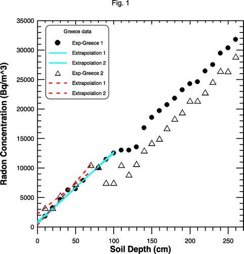
Figure 1. The experimental radon profile with soil depth for Greece 1 and Greece 2 data and radon experimental extrapolation to soil surface.

The radon concentration data for Greece in 2002–2003 was used to calibrate the model unknown coefficients especially the radon transfer coefficient, h, and the measured data in 2003–2004 to test its validity. The surface radon concentration, C (at node 1) and the surface radon flux q₀ are calculated or produced by the model. A value for h = 0.0002 cm/s was found sufficient for all the numerical runs in this study.

4.2. Numerical model results for Greece’s data

In the past it has been assumed that the soil radon concentrations with depth exhibit a one curve pattern. Treating the soil as a one homogeneous layer does not match the radon measured field profiles where sudden breaks appear clearly in the radon profiles as seen in Figure 1, leading to questioning the soil homogeneous assumption. The FEM calculations for the diffusion advection decay equation using the radon soil–air transfer coefficient, h = 0.0002 cm s⁻¹, and the multi-layer pattern is found to be in good agreement with the field data as seen in Figure 2(a) and (b). The numerical and field data for Greece 1 and Greece 2 are shown in Figure 2(a) and (b), respectively. The soil in this area is sand and clay with different composition ratio and this ratio is changing along the soil depth. The calculations using two and three layers assumption is showing better agreement with the field data than the one layer assumption where each layer was assigned a certain diffusion coefficient (D₁, D₂, and D₃) given in Table 2. The layer borders in both Figure 2(a) and (b) may not be exact but different layers trend is clear in both figures. The very good agreement between the simulated and measured values highlights the good calibration of the radon transport model. The multi-layered behavior stated previously (Antonopoulos-Domis et al., 2009; Yakovleva & Parovik, 2010) is confirmed by the present work. It was found in Figure 2(a) and (b) that the diffusion coefficient for the first, top layer (0–50 cm) is always low compared to other layer values, while the D₃ values for the deepest layer is in general greater than the layers above. The variation of different diffusion coefficients with soil depth for Greece data is shown in Table 2 and Figure 6. Soil depth in Figure 6 is taken to be the lower border of a given layer. The correlation value, R², is found to be 0.691 and consequently the linear correlation coefficient r = 0.831 showing strong linear relation between the diffusion coefficient and soil depth. The calculated soil surface radon concentrations and fluxes are given in Table 3. Surface flux values of 1.68 mBq m⁻² s⁻¹ and 3.17 mBq m⁻² s⁻¹ are predicted by the model in Greece 1 and Greece 2, respectively. The calculated surface radon concentrations by the model are in excellent agreement with the measured values obtained by extrapolation (Figure 1). For Greece 1, the model predicts soil–air surface radon concentration of 850 Bq m⁻³ which falls within the range of the extrapolated values (550–950 Bqm⁻³). For Greece 2, the model predicts soil–air surface radon concentration of 1,640 Bq m⁻³ which also falls within the range of the extrapolated values (from 300 to 2,200 Bq m⁻³).

Figure 2. (a) and (b) The experimental radon profile with soil depth for Greece 1 and Greece 2 data, respectively, compared to the model calculations using one, two, and three-layered assumptions.

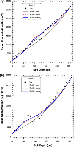
Table 2. The effective diffusion coefficient, D (cm² s⁻¹) of radon in natural soil for the different layers calculated for some countries

Country	Region	Data	1-Layer	2-Layers		3-Layers
			D1	D1	D2	D1	D2	D3
Greece	Greece 1		0.085	0.030	0.080	0.025	0.048	0.085
	Greece 2		0.070	0.035	0.075	0.030	0.090	0.070
Germany-Seik	BT-1			0.005	0.019
	BT-2			0.002	0.027
	FT-1			0.013	0.032
	FT-2			0.012	0.027
South Africa	M 1			0.003	0.016
	M 2			0.003	0.022
Jordan	AHP-Summer			0.0015	0.0120
	AHP-Winter			0.0015	0.0100
	Basalt-Summer			0.0030	0.0250
	Basalt-Winter			0.0030	0.0200

Table 3. The calculated soil surface radon concentration, C_o (Bq m⁻³) and radon surface flux, q_o (mBq m⁻² s⁻¹) for the different countries

Data		Co field data** (Bq m^−3)	Co Model (Bq m^−3)	Radon flux (mBqm^−2 s^−1)
Greece	Greece 1	550–950	850	1.68
	Greece 2	300–2,200	1,640	3.17
Germany-Seik	BT-1	NA^*	350	0.70
	BT-2	NA	103	0.21
	FT-1	1,000	1,025	2.05
	FT-2	NA	940	1.88
South Africa	M 1	NA	710	1.42
	M 2	NA	3,525	7.05
Jordan	AHP-Summer	3,000	3,320	6.64
	AHP-Winter	2,000	2,730	5.46
	Basalt-Summer	4,000	4,115	8.23
	Basalt-Winter	2,500	2,390	4.78

^* Not Available.

^** Extrapolated linearly from the radon concentrations close to the soil surface.

4.3. Numerical model results for Germany’s data

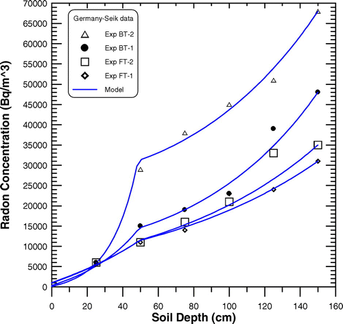
The numerical study shows its success in matching the measured radon profiles in the Germant-Seik area as illustrated in Figure 3. The radon profile measured for depths down to 150 cm shows increasing radon concentration with depth. The soil composition in this area consists of sand, gravels, and clay. As observed for the Greece data before, the two-layered pattern is also observed and the top layer shows less diffusion coefficient compared to the deeper one, Table 2. Field data, in this case allow for extrapolation only for the case of Exp FT-1 with extrapolated radon concentration of about 1,000 Bq m⁻³ while the model predicts a value of 1,025 Bq m⁻³ which indicated success of the model. This causes difficulty in comparing the calculated radon surface concentrations with the measured ones but visual comparisons from Figure 3 confirm that the model surface values approach the visually extrapolated field values. Table 3 shows the calculated soil surface radon fluxes which exhibit low values in accordance with low radon surface values.

Figure 3. The experimental radon profile with soil depth and two-layered model calculation for Germany-Seik data.

4.4. Numerical model results for South Africa’s data

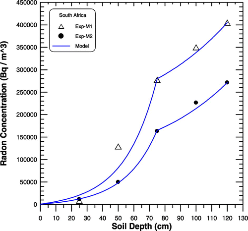
The finite element model predictions and the corresponding data for mine tailings M 1 and M 2 at depths 25, 50, 75, 100, and 120 cm are shown in Figure 4. The soil samples collected at different depths show appreciable differences in radon concentration with depth suggesting that more radon is being transported deeper in the dump. The radon transport and diffusion for this data was studied using a suitable diffusion coefficient in each layer to obtain the best correlation between measured and numerical profiles. As observed for the Greek and German data, the radon profile in the mine waste area shows two-layer behavior. Also, the top surface layer shows less diffusion coefficient compared to the deepest one. Table 2 shows the diffusion coefficients while Table 3 shows the soil surface radon fluxes and concentrations. Extrapolation is not possible for obtaining the radon surface concentration in this case.

Figure. 4. The experimental radon profile with soil depth and two-layered model calculation for South Africa data.

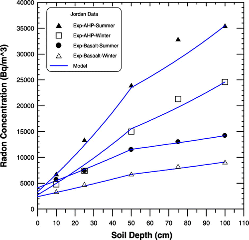
4.5. Numerical model results for Jordan’s data

This data has the property that it gives summer as well as winter radon profiles for a given geophysical location. The radon depth profile for both cases shows the existence of the two-layered pattern as illustrated in Figure 5. In summer, the radon exhalation rate is higher than winter. The first layer gives the least D-value compared to the second layer in agreement with the previous findings. Table 2 shows the diffusion coefficients while Table 3 shows the radon surface concentration and the soil surface radon flux. Relatively higher radon fluxes are observed from Table 3 with a maximum flux of 8.23 mBq m⁻² s⁻¹. Table 3 also shows the excellent agreement between the predicted model and measured soil–air surface radon concentrations in the four cases.

Figure 5. The experimental radon profile with soil depth and two-layered model calculation for Jordan data.

5. Discussion

The present investigation deals with field data in which the soil depths ranges from 100 to 260 cm. It is seen from the data in the different figures that at this relatively small depths, the radon profile is increasing with depth but saturation conditions are not reached yet. The objective of this study is to simulate radon distribution under field conditions and not to make comparisons with analytical solutions of radon in soils with theoretically infinite depth.

The two and three-layered radon profile found in numerical analysis for Greece 1, Figure 2(a), can be explained in terms of soil particle distribution and the possible compaction of the soil. Antonopoulos-Domis et al. (2009) reported different soil layers of different clay and sand compositions. In the first 50 cm layer, sand is more dominant than clay. Different soil matrix at depth of about 60–80 cm was found where sand and clay concentrations remain practically constant. For depths higher than 100 cm, there is an inversion of the curves where clay concentration becomes higher than sand. All these lead to different soil compaction, grain size, and soil porosity along the considered soil column. The multi-layered pattern is also confirmed by observing a similar pattern in the same place when it was studied in the following year, Greece 2 data. This finding can also be supported by the multi-layered behavior of the radon migration profile observed in the German, South African, and Jordanian data. For these regions similar radon patterns were observed, despite the different geophysical locations with different soil formations and different meteorological conditions. The multi-layered pattern was confirmed in all data under investigation with different diffusion coefficients.

The radon transport equation was solved often in the past using the assumption that the diffusion coefficient, D is depth independent (Dörr & Münnich, 1990). The present finding does not support this assumption as illustrated in Table 2 and Figure 6. The diffusion coefficient shows variations with depth where D₂ and D₃ have higher values than the D₁-values. The diffusion coefficients variation with soil depth can be explained in terms of the continuity of the radon flux at soil interfaces where there is a change in the soil type. At a soil interface where there is a change in soil type the slope or the concentration gradient changes and consequently the diffusion coefficient simultaneously changes to keep a constant flux along that soil interface.

Figure 6. The diffusion coefficient as a function of the soil depth for Greece data.

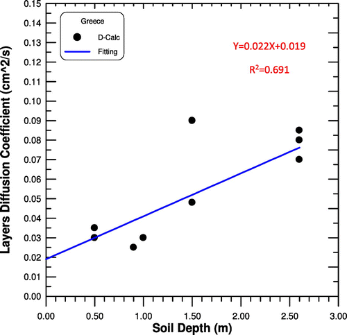
Table 2 shows the different diffusion coefficients D (cm² s⁻¹) for the different countries. The corresponding calculated diffusion length, L is between 27 and 207 cm in agreement with previous findings (L = 24–213 cm) (Hosoda et al., 2009; Prasad et al., 2012). The top surface layer might be affected by the atmospheric pressure, which suppresses the diffusion of radon upward and reduce the migration distance. This might explain the small values of surface radon fluxes. Soil humidity appears as the decisive factor in radon release values. Generally, the presence of water in soil produces a reduction of soil porosity and consequently a diminution in gas diffusion rates, in particular, in the top decimeter of soil. This retards ²²²Rn release and increases the concentration of ²²²Rn in the top layer near the soil-atmosphere surface (Dueñas et al., 1997). The diffusion coefficient D₁ in the first layer is also dependent on the moisture content and soil humidity. It’s well known that water in soil pore will reduce ²²²Rn diffusion coefficient (Andersen, 2001; Rogers & Nielson, 1991).

Radon diffusion and emanation is unsteady as well as seasonally affected. Radon release in summer time is higher than winter as revealed in the Jordanian field data and the numerical results. A positive correlation has been found between soil temperature and radon emanation power (Iskandar et al., 2004). When the temperature of the top surface is high, the soil humidity is low and consequently ²²²Rn release would be greater than when the temperature of the top soil is low. Winter time is a situation associated with negative thermal gradients linked generally to high soil humidity.

One of the objectives of this paper is to determine the soil–air interface flux using the radon transfer coefficient, h, where its value has been determined as 0.0002 cm/s. It is noted that this value is twice the widely reported advective velocity of 0.0001 cm/s. After determining h, the radon flux can be calculated using Equation (4). Table 3 compiles the calculated radon concentration at the surface and the surface radon fluxes. From this table, one can observe that summer radon exhalation rates are higher than winter. On the soil surface, the calculated radon flux, as shown in Table 3, varied from 0.2 to 8.2 mBq m⁻² s⁻¹ compared to the world average values of 7 to 38 mBq m⁻² s⁻¹ (Nazaroff, 1992; Richon et al., 2010; Sahoo et al., 2011). Antonopoulos-Domis et al. (2009) using their two-layers analytically based model found a radon concentration at the soil surface (C_soil (z = 0)) for Greece 1 data equals to 90 Bq m⁻³ while field values obtained through extrapolation were between 550 and 950 Bq m⁻³. The present numerical model predicts a corresponding surface radon concentration of 850 Bq m⁻³ which lies within this range. The numerical model provides values for radon concentration below the soil surface that are difficult to be measured. The fact that all field data reported in this study do not show the radon concentration just below or at the soil surface highlights the contribution of numerical modeling to provide for these extremely important surface radon fluxes and concentrations.

6. Conclusions

Radon transport through natural soils exhibits a multi-layer behavior. Each layer has its own diffusion coefficient depending on its soil structure as well as meteorological parameters. To summarize one can conclude that:

•	Numerical study of field data is fruitful where the field data becomes more readable using numerical techniques.
•	The Finite Element Method shows its flexibility and power for studying the multi-layer phenomena of the radon diffusion and in incorporating flux type convective boundary conditions deviating from the standard assumption of zero soil surface concentration boundary conditions.
•	Radon profile distribution behavior is not monotonic.
•	Diffusion coefficient in natural soil is a geophysical parameter, differs from one location to another.
•	Multi-layer behavior of the radon profile is confirmed in all the considered locations.
•	The first layer shows low diffusion coefficient in almost all the considered profiles, which can be explained in terms of moisture and water content as well as atmospheric pressure.
•	Deeper layers show higher diffusion coefficients and higher diffusion lengths which can be explained by its dryness.
•	The diffusion coefficient is soil depth dependent and it is a local property depending on the soil composition and soil matrix meteorological conditions.
•	Radon soil–air transfer coefficient, h, that is needed for surface flux calculation can be taken as 0.0002 cm/s.

Additional information

Funding

Funding. The authors received no direct funding for this research.

Notes on contributors

Youssef I. Hafez

Youssef Hafez graduated in 1984 from Cairo University at the Civil Engineering Department. Soon after, he joined the Nile Research Institute, Egypt. He got both the Master of Science in 1990 and the PhD in 1995 at Colorado State University, USA, in Civil Engineering. The PhD topic was about turbulence modeling in closed and open channels using the Finite Element numerical method. In 2004 and till now, Hafez has joined the Royal Commission Colleges and Institutes in Yanbu in Saudi Arabia. Hafez’s research interests include applying numerical methods such as the finite elements to model and solve real-life practical problems in fluid mechanics, hydraulics, dynamics, and environmental engineering.

El-Sayed Awad

El-Sayed Awad works now at Physics Department, Faculty of Science, Menoufia University, Shibin El-Koom, Egypt. Awad joined the Royal Commission Colleges and Institutes in Yanbu in Saudi Arabia from 2004 until 2015. Awad’s research interests include radiation physics and radon studies.

References

- Al-Shereideh, S. A., Bataina, B. A., & Ershaidat, N. M. (2006). Seasonal variations and depth dependence of soil radon concentration levels in different geological formations in Deir Abu-Said District, Irbid—Jordan. Radiation Measurements, 41, 703–707.10.1016/j.radmeas.2006.03.004
- Andersen, C. E. (2001). Numerical modelling of radon-222 entry into houses: An outline of techniques and results. Science of The Total Environment, 272, 33–42.10.1016/S0048-9697(01)00662-3
- Antonopoulos-Domis, M., Xanthos, S., Clouvas, A., & Alifrangis, D. (2009). Experimental and theoretical study of radon distribution in soil. Health Physics, 97, 322–331.10.1097/HP.0b013e3181adc157
- Clouvas, A., Leontaris, F., Xanthos, S., & Alifragis, D. (2016, September 24). Radon migration in soil and its relation to terrestrial gamma radiation in different locations of the greek early warning system network. Radiat Prot Dosimetry doi:10.1093/rpd/ncw277
- Dörr, H., & Münnich, K. O. (1990). 222Rn flux and soil air concentration profiles in West_Geramny. Soil 222Rn as tracer for gas transport in the unsaturated soil zone, Tellus B, 42, 20–28.
- Dueñas, C., Fernández, M. C., Carretero, J., & Liger, E. (1996). Measurement of 222Rn in soil concentrations in interstitial air. Applied Radiation and Isotopes, 47, 841–847.
- Dueñas, C., Fernández, M. C., Carretero, J., Liger, E., & Pérez, M. (1997). Release of 222Rn from some soils. Annales Geophysicae, 15, 124–133.
- Fournier, F., Groetz, J. E., Jacob, F., Crolet, J. M., & Lettner, H. (2005). Simulation of radon transport through building materials: influence of the water content on radon exhalation rate. Transport in Porous Media, 59, 197–214.10.1007/s11242-004-1489-0
- Hafez, Y. (1995). A k-ε Turbulence model for predicting the three-dimensional velocity field and boundary shear in open and closed channels ( Ph.D Dissertation). Civil Engineering Department, Colorado State University, Fort Collins, CO.
- Hosoda, M., Tokonami, S., Sorimachi, A., Janik, M., Ishikawa, T., Yatabe, Y., & Yamada, J. (2009). Experimental system to evaluate the effective diffusion coefficient of radon. Review of Scientific Instruments, 80, 013501–013505.10.1063/1.3049379
- Iskandar, D., Yamazawa, H., & Iida, T. (2004). Quantification of the dependency of radon emanation power on soil temperature. Applied Radiation and Isotopes, 60, 971–973.10.1016/j.apradiso.2004.02.003
- Jiranek, M., & Svoboda, Z. (2009). Transient radon diffusion through radon-proof membranes: A new technique for more precise determination of the radon diffusion coefficient. Building and Environment, 44, 1318–1327.10.1016/j.buildenv.2008.09.017
- Künze, N., Koroleva, M., & Reuther, C. D. (2013). Soil gas 222Rn concentration in northern Germany and its relationship with geological subsurface structures. Journal of Environmental Radioactivity, 115, 83–96.10.1016/j.jenvrad.2012.07.009
- Liu, G., & Si, B. C. (2009). Multi-layer diffusion model and error analysis applied to chamber-based gas fluxes measurements. Agricultural and Forest Meteorology, 149, 169–178.10.1016/j.agrformet.2008.07.012
- Nazaroff, W. W. (1992). Radon transport from soil to air. Reviews of Geophysics, 30, 137–160.10.1029/92RG00055
- Nazaroff, W. W., & Nero, A. V. (1988). Radon and Its Decay Products in Indoor Air. New York, NY: McGraw-Hill.
- Olise, F. S., Akinnagbe, D. M., & Olasogba, O. S. (2016). Radionuclides and radon levels in soil and ground water from solid minerals-hosted area, south-western Nigeria. Cogent Environmental Science, 2, 1142344.
- Papp, B., Deák, F., Horváth, Á., Kiss, Á., Rajnai, G., & Szabó, C. (2008). A new method for the determination of geophysical parameters by radon concentration measurements in bore-hole. Journal of Environmental Radioactivity, 99, 1731–1735.
- Prasad, G., Ishikawa, T., Hosoda, M., Sorimachi, A., Janik, M., Sahoo, S. K., … Uchida, S. (2012). Estimation of radon diffusion coefficients in soil using an updated experimental system. Review of Scientific Instruments, 83, 093503–093508.10.1063/1.4752221
- Richon, P., Klinger, Y., Tapponnier, P., Li, C., Van Der Woerd, J. V., & Perrier, F. (2010). Measuring radon flux across active faults: Relevance of excavating and possibility of satellite discharges. Radiation Measurements, 45, 211–218.10.1016/j.radmeas.2010.01.019
- Rogers, V. C., & Nielson, K. K. (1991). Correlations for predicting air permeabilities and 222Rn diffusion coefficients of soils. Health Physics, 61, 225–230.10.1097/00004032-199108000-00006
- Ryzhakova, N. K. (2012). Parameters of modeling radon transfer through soil and methods of their determination. Journal of Applied Geophysics, 80, 151–157.10.1016/j.jappgeo.2012.01.010
- Sahoo, B. K., & Mayya, Y. S. (2010). Two dimensional diffusion theory of trace gas emission into soil chambers for flux measurements. Agricultural and Forest Meteorology, 150, 1211–1224.10.1016/j.agrformet.2010.05.009
- Sahoo, B. K., Sapra, B. K., Gaware, J. J., Kanse, S. D., & Mayya, Y. S. (2011). A model to predict radon exhalation from walls to indoor air based on the exhalation from building material samples. Science of The Total Environment, 409, 2635–2641.10.1016/j.scitotenv.2011.03.031
- Savović, S., Djordjevich, A., Tse, P. W., & Krstić, D. (2011a). Radon diffusion in an anhydrous andesitic melt: a finite difference solution. Journal of Environmental Radioactivity, 102, 103–106.10.1016/j.jenvrad.2010.10.009
- Savović, S., Djordjevich, A., Tse, P. W., Nikezić, D., & Nikezić, D. (2011b). Explicit finite difference solution of the diffusion equation describing the flow of radon through soil. Applied Radiation and Isotopes, 69, 237–240.10.1016/j.apradiso.2010.09.007
- Savovic, S., Djordjevich, A., & Ristic, G. (2012). Numerical solution of the transport equation describing the radon transport from subsurface soil to buildings. Radiation Protection Dosimetry, 150, 213–216.10.1093/rpd/ncr397
- Shitrit, Y., Dody, A., Alfassi, Z. B., & Berant, Z. (2012). Measurement of 222Rn diffusion through sandy soil with solar cells photodiodes as the detector. Journal of Environmental Radioactivity, 105, 1–5.10.1016/j.jenvrad.2011.10.005
- Speelman, W. J. (2004). Modelling and measurement of radon diffusion through soil for application on mine tailings dams ( Msc thesis). Faculty of natural Sciences, University of Western Cape, South Africa.
- Thompson, E. G. (2005). Introduction to the finite element method, theory, programming, and applications (5th ed.). Hoboken, NJ: John Wiley & Sons.
- Urošević, V., & Nikezić, D. (2003). Radon transport through concrete and determination of its diffusion coefficient. Radiation Protection Dosimetry, 104, 65–70.
- World Health Organization. (2009). WHO Handbook on Indoor Radon. Retrieved from http://whqlibdoc.who.int/publications/2009/9789241547673_eng.pdf
- Yakovleva, V. S., & Parovik, R. I. (2010). Solution of diffusion-advection equation of radon transport in many-layered geological media. Nukleonika, 55, 601–606.