Closed form solutions of complex wave equations via the modified simple equation method

Abstract

The Kundu–Eckhaus equation and the derivative nonlinear Schrodinger equation describe various physical processes in nonlinear optics, plasma physics, fluid mechanics, magneto-hydrodynamic equation in the presence of the Hall Effect. Thus, closed form solutions of these equations are very important to realize the obscurity of the phenomena. The modified simple equation (MSE) method is highly effective and competent mathematical tool to examine closed form wave solutions of nonlinear evolution equations (NLEEs) arising in mathematical physics, applied mathematics and engineering. In this article, the MSE method is suggested and executed to construct closed form wave solutions of the above-mentioned equations involving parameters. When the parameters receive special values, impressive solitary wave solutions are derived from the exact solutions.

Keywords:

• modified simple equation (MSE) method
• Kundu–Eckhaus equation
• derivative nonlinear Schrodinger equation
• nonlinear evolution equations (NLEEs)
• closed form wave solutions

Public Interest Statement

Non-linear evolution equations (NLEEs) frequently arise in formulating fundamental laws of nature and in mathematical analysis of a wide variety of problems naturally arising from meteorology, solid-state physics, fluid dynamics, plasma physics, ocean and atmospheric waves, material science, etc. Closed form solutions to NLEEs play a significant role in nonlinear science, especially in nonlinear physical science, since it can provide much physical information and more insight into the physical aspects of the problem. As a result, numerous techniques have been developed by several groups of mathematicians and physicists to examine closed form solutions to NLEEs. In this article, we use the modified simple equation method to extract fresh and further general exact traveling wave solutions to the Kundu–Eckhaus equation and derivative nonlinear Schrodinger equation. Thus, we obtain abundant closed form wave solutions of these two equations among them some are new solutions. We expect that the new exact traveling wave solutions will be helpful to illuminate the connected phenomena.

1. Introduction

Nonlinear evolution equations (NLEEs) and their closed form solutions are widely used to describe the inner mechanism and obscurity of complex phenomena in various fields of science and engineering. NLEEs appear in broad range of scientific research in various fields, such as plasma physics, high energy physics, nuclear physics, optical fibers, fluid dynamics, solid-state physics, fluid mechanics, biomechanics, gas dynamics, elasticity, chemical reactions, geochemistry, biochemistry, meteorology, etc. By the aid of closed form solutions, when exist, the phenomena modeled by NLEEs can be better understood. Hence it is very essential to search for further closed form traveling solutions to NLEEs to access the phenomena thoroughly. Therefore, the study of the traveling wave solutions for NLEEs plays a significant role in the study of nonlinear complex phenomena. But till now there is no unique method to examine all kinds of NLEEs. As a result, different groups of mathematicians, physicist, and engineers have been working tirelessly to develop effective methods for obtaining close form solutions to NLEEs. For this reason, in recent years several methods have been established to search exact solution, such as the homogeneous balance method (Wang, 1995; Zayed, Zedan, & Gepreel, 2004), the tanh-function method (Nassar, Abdel-Razek, & Seddeek, 2011), the Hirota’s bilinear transformation method (Hirota, 1973; Hirota & Satsuma, 1981), the Jacobi-elliptic function expansion method (Chen & Wang, 2005; Liu, Fu, Liu, & Zhao, 2001), the nonlinear transform method (Yang, Liu, & Yang, 2001), the extended tanh-method (Abdou, 2007; Fan, 2000), the Exp-function method (Akbar & Ali, 2011; Bekir & Boz, 2008; Naher, Abdullah, & Akbar, 2011, 2012), the first integration method (Taghizadeh & Mirzazadeh, 2011), the Painleve expansion method (Weiss, Tabor, & Carnevale, 1982), the complex hyperbolic function method (Chow, 1995; Wang & Zhou, 2003), the F-expansion method (Sirendaoreji, 2004), the functional variable method (Çevikel, Bekir, Akar, & San, 2012), the Adomian decomposition method (Adomian, 1994), the modified Exp-function method (He, Li, & Long, 2012), the auxiliary equation method (Sirendaoreji, 2004), the sine-cosine method (Wazwaz, 2004), the generalized Riccati equation method (Yan & Zhang, 2001), the Lie group symmetry method (Guo & Lin, 2010), the exp(−Φ(η))-expansion method (Islam, Alam, Sazzad Hossain, Roshid, & Akbar, 2013; Khan & Akbar, 2013a), the perturbation method (Biswas, Zony, & Zerrad, 2008), the (G^′/G)-expansion method (Akbar, Ali, & Mohyud-Din, 2012; Akbar, Ali, & Zayed, 2012; Alam, Akbar, & Roshid, 2013; Manafianheris, 2012; Neyrame, Roozi, Hosseini, & Shafiof, 2010; Zayed & Shorog, 2013), the asymptotic method (He, 2008), the improve (G′/G)-expansion method (Zhang, Jiang, & Zhao, 2010), the modified simple equation method (Akter & Ali Akbar, 2015; Jawad, Petković, & Biswas, 2010; Khan & Akbar, 2013b; Khan, Akbar, & Ali, 2013; Zayed & Ibrahim, 2012), etc. The recently developed modified simple equation method is getting popularity in use because of its straightforward calculation procedure and there is no need of the symbolic computation software to manipulate the algebraic equations.

The objective of this article is to introduce and implement the modified simple equation method to extract further general and some fresh exact traveling wave solutions to the Kundu–Eckhaus equation and derivative nonlinear Schrodinger equation. The rest of the article is arranged as follows: In Section 2, modified simple equation method is discussed. In Section 3, the MSE method is applied to examine the NLEEs indicated above. In Section 4, results and discussion are adjoined. In Section 5 conclusions are provided.

2. Analysis of the modified simple equation method

To describe the modified simple equation method, let us consider a nonlinear evolution equation in two independent variables x and t in the form:

(2.1) $$F\left(u,u_t,u_x,u_{tt},u_{xx},u_{xt,}\dots \right)=0,$$(2.1)

where u = u(x, t) is an unknown function and F is a polynomial of u(x, t) and its partial derivatives wherein the highest order derivatives and nonlinear terms are involved and the subscripts are used for partial derivatives. The fundamental steps of this method are presented in the following:

Step 1: Initiating a compound variable $\mathit{\xi }$, we combine the real variables x and t in this way:

(2.2) $$u\left(x,t\right)=u\left(\mathit{\xi }\right),\mathit{\xi }=x\pm \mathit{\omega }t,$$(2.2)

where ω is the celerity of the traveling wave.

The traveling wave transformation (2.2) permits us in reducing Equation (2.1) into an ODE for $u=u\left(\mathit{\xi }\right)$ in the form:

(2.3) $$G\left(\text{u,}{u}^{\prime },u^{″},u^{″\prime }\dots \right)=0,$$(2.3)

where G is a polynomial in $u\left(\mathit{\xi }\right)$ and its derivatives, the prime indicates the derivative with respect to ξ.

Step 2: Assume the solution of (2.3) which can be expressed of the form:

(2.4) $$u\left(\mathit{\xi }\right)=\sum _{i=0}^N{a}_i{\left(\frac{{\mathit{\psi }}^{\prime }(\mathit{\xi })}{\mathit{\psi }(\mathit{\xi })}\right)}^i$$(2.4)

where $a_i\left(i=0,1,2,3,\dots N\right)$ are arbitrary constants to be determined such that a_N ≠ 0 and ψ(ξ) is an unknown function to be assessed later, such that ${\mathit{\psi }}^{\prime }\left(\mathit{\xi }\right)\ne 0$. The characteristic and uniqueness of this method is that, ψ(ξ) is not known function or not a solution of any uncomplicated equation, whereas in the Exp-function method, (G′/G)-expansion method, Jacobi elliptic function method, tanh-function method, sine-cosine method, etc. the solution are proposed in terms of known function. Therefore, it might be possible to get some new solution by this method (Khan & Akbar, 2013b).

Step 3: We determine the positive integer N occurs in (2.4) by balancing the order of linear and nonlinear terms appearing in (2.3).

Step 4: Compute the necessary derivatives $u^{\prime },u^{″},\dots$ and insert Equations (2.4) into (2.3) and then we account the function $\mathit{\psi }(\mathit{\xi })$. The above procedure makes a polynomial in (1/ψ(ξ)). Equating the coefficients of same power of this polynomial to zero, yields a system of algebraic and differential equations that can be solved to find $a_i\left(i=0,1,2,3,\dots N\right)$ and $\mathit{\psi }(\mathit{\xi })$. This completes the determination of solutions of Equation (2.1).

3. Applications of the method

In this section, the modified simple equation method (MSE) has been put to use to examine the closed form solutions leading to solitary wave solutions to the Kundu–Eckhaus equation and derivative nonlinear Schrodinger equation.

3.1. Example 1

Let us consider the Kundu–Eckhaus equation in the form (Levko & Volkov, 2006):

(3.1) $$i{u}_t+u_{xx}-2\mathit{\sigma }{\left|u\right|}^{2}u+{\mathit{\delta }}^2{\left|u\right|}^{4}u+2i\mathit{\delta }{({\left|u\right|}^2)}_{x}u=0.$$(3.1)

The Kundu–Eckhaus equation describes various physical processes, as for instance nonlinear optics, plasma physics, fluid mechanics, etc. It is connected to the mixed nonlinear Schrodinger equation by gauge function and alterable to different types of known integrable equations, such as nonlinear Schrodinger equation (NLSE), derivative NLSE, higher derivative NLSE, Chen-Lee-Liu-Gerjikov-Vanov equation, etc. for a variety of choices of the parameters. This equation is linked with conserved quantity, Lax pair, closed form soliton solution, rogue wave, etc.

The complex transformations $u\left(x,t\right)=e^{i\left(\mathit{\alpha }x+\mathit{\beta }t\right)}u\left(\mathit{\xi }\right),\mathit{\xi }=ik\left(x-\mathit{\omega }t\right)$, where k and ω are constants, converts Equation (3.1) into an ODE of the form,

(3.2) $$\left({\mathit{\alpha }}^2+\mathit{\beta }\right)u+k\left(\mathit{\omega }+2\mathit{\alpha }\right)u^{\prime }+k^2{u}^{\prime \prime }+2\mathit{\sigma }{u}^3-{\mathit{\delta }}^2{u}^5+4k\mathit{\delta }{u}^2{u}^{\prime }=0.$$(3.2)

Balancing the order of nonlinear and linear terms u⁵ and u″, respectively, yields(3.3) $$N+2=5N\Rightarrow N=1/2$$(3.3)

To find a polynomial type closed form solution, N should be an integer. This requires the use of the transformation(3.4) $$u\left(\mathit{\xi }\right)=v{\left(\mathit{\xi }\right)}^{\frac{1}{2}}$$(3.4)

This transformation converts Equation (3.2) to the following equation:(3.5) $$4\left({\mathit{\alpha }}^2+\mathit{\beta }\right)v^2+2k\left(\mathit{\omega }+2\mathit{\alpha }\right)v{v}^{\prime }+2k^{2}v{v}^{\prime \prime }-k^2{v}^{\prime 2}+8\mathit{\sigma }{v}^3-4{\mathit{\delta }}^2{v}^4+8k\mathit{\delta }{v}^2{v}^{\prime }=0$$(3.5)

Balancing the order of vv″ and v⁴, yields N = 1.

Therefore, the solution of Equation (3.5) becomes,

(3.6) $$v=a_0+a_1\left(\frac{{\mathit{\psi }}^{\prime }}{\mathit{\psi }}\right),$$(3.6)

where a₀ and a₁ are constants, such that a₁ ≠ 0 and ψ(ξ) is an unknown function to be calculated. Substituting (3.6) and its derivatives into (3.5) and then equating the coefficients of ψ⁰, ψ⁻¹, ψ⁻², ψ⁻³, ψ⁻⁴ to zero we achieve the successive algebraic and differential equations,

(3.7) $$4{\mathit{\alpha }}^2{a}_0^2+4\mathit{\beta }{a}_0^2-4{\mathit{\delta }}^2{a}_0^4+8\mathit{\sigma }{a}_0^3=0$$(3.7) (3.8) $$4k\mathit{\alpha }{a}_0{a}_1{\mathit{\psi }}^{\prime \prime }+8k\mathit{\delta }{a}_0^2{a}_1{\mathit{\psi }}^{\prime \prime }+2k\mathit{\omega }{a}_0{a}_1{\mathit{\psi }}^{\prime \prime }+8{\mathit{\alpha }}^2{a}_0{a}_1{\mathit{\psi }}^{\prime }-16{\mathit{\delta }}^2{a}_0^3{a}_1{\mathit{\psi }}^{\prime }+2k^2{a}_0{a}_1{\mathit{\psi }}^{″\prime }+24\mathit{\sigma }{a}_0^2{a}_1{\mathit{\psi }}^{\prime }+8\mathit{\beta }{a}_0{a}_1{\mathit{\psi }}^{\prime }=0$$(3.8) (3.9) $$\begin{array}{c}2k^2{a}_1^2{\mathit{\psi }}^{\prime }{\mathit{\psi }}^{″\prime }+4\mathit{\beta }{a}_1^2{\mathit{\psi }}^{\prime 2}-8k\mathit{\delta }{a}_0^2{a}_1{\mathit{\psi }}^{\prime 2}+2k\mathit{\omega }{a}_1^2{\mathit{\psi }}^{\prime }{\mathit{\psi }}^{″}+24\mathit{\sigma }{a}_0{a}_1^2{\mathit{\psi }}^{\prime 2}\hfill \\ -2k\mathit{\omega }{a}_0{a}_1{\mathit{\psi }}^{\prime 2}-6k^2{a}_0{a}_1{\mathit{\psi }}^{\prime }{\mathit{\psi }}^{″}-k^2{a}_1^2{\mathit{\psi }}^{″2}-4k\mathit{\alpha }{a}_0{a}_1{\mathit{\psi }}^{\prime 2}+4k\mathit{\alpha }{a}_1^2{\mathit{\psi }}^{\prime }{\mathit{\psi }}^{″}\hfill \\ +16k\mathit{\delta }{a}_0{a}_1^2{\mathit{\psi }}^{\prime }{\mathit{\psi }}^{″}+4{\mathit{\alpha }}^2{a}_1^2{\mathit{\psi }}^{\prime 2}-24{\mathit{\delta }}^2{a}_0^2{a}_1^2{\mathit{\psi }}^{\prime 2}=0\hfill \end{array}$$(3.9) (3.10) $$4k^2{a}_0{a}_1{\mathit{\psi }}^{\prime 3}-16{\mathit{\delta }}^2{a}_0{a}_1^3{\mathit{\psi }}^{\prime 3}+8k\mathit{\delta }{a}_1^3{\mathit{\psi }}^{\prime 2}{\mathit{\psi }}^{″}-4k^2{a}_1^2{\mathit{\psi }}^{\prime 2}{\mathit{\psi }}^{″}-16k\mathit{\delta }{a}_0{a}_1^2{\mathit{\psi }}^{\prime 3}+8\mathit{\sigma }{a}_1^3{\mathit{\psi }}^{\prime 3}-2k\mathit{\omega }{a}_1^2{\mathit{\psi }}^{\prime 3}-4k\mathit{\alpha }{a}_1^2{\mathit{\psi }}^{\prime 3}=0$$(3.10)

(3.11) $$8k\mathit{\delta }{a}_1^3{\mathit{\psi }}^{\prime 4}+3k^2{a}_1^2{\mathit{\psi }}^{\prime 4}-8{\mathit{\delta }}^2{a}_1^4{\mathit{\psi }}^{\prime 4}=0$$(3.11)

From Equation (3.7), we obtain a₀ = 0 and $\frac{\mathit{\sigma }\pm p}{{\mathit{\delta }}^2}$, where $p=\sqrt{{\mathit{\sigma }}^2+({\mathit{\alpha }}^2+\mathit{\beta }){\mathit{\delta }}^2}$.

And from Equation (3.11), we achieve $a_1=\frac{\left(-2\pm \sqrt{7}\right)k}{2\mathit{\delta }},$ since a₁ ≠ 0.

From Equation (3.10), it can be deduced that(3.12) $$\frac{{\mathit{\psi }}^{″}}{{\mathit{\psi }}^{\prime }}=\mathit{\lambda }$$(3.12) (3.13) $$\text{where}\mathit{\lambda }=\frac{(4k^2{a}_0{a}_1-16{\mathit{\delta }}^2{a}_0{a}_1^3-16k\mathit{\delta }{a}_0{a}_1^2+8\mathit{\sigma }{a}_1^3-2k\mathit{\omega }{a}_1^2-4k\mathit{\alpha }{a}_1^2)}{\left(4k^2{a}_1^2-8k\mathit{\delta }{a}_1^3\right)}$$(3.13)

Integrating (3.12) with respect to ξ, yields(3.14) $${\mathit{\psi }}^{\prime }=c_1{\text{e}}^{\mathit{\lambda }\mathit{\xi }}$$(3.14) (3.15) $$\text{and}\mathit{\psi }=\frac{c_1{\text{e}}^{\mathit{\lambda }\mathit{\xi }}}{\mathit{\lambda }}+c_2$$(3.15)

where c₁ and $c_2$ are arbitrary constants.

Case 1: When $a_0=0$ and $a_1=\frac{\left(-2\pm \sqrt{7}\right)k}{2\mathit{\delta }}$, solving Equation (3.9) by using (3.13–3.15), provides ω and $\mathit{\lambda }$. Then by using the values of a₀, a₁, ω, and $\mathit{\lambda }$, yields $v\left(\mathit{\xi }\right)=\frac{1}{{\mathit{\delta }}^2}\left(\frac{c_1\left(\mathit{\sigma }\pm p\right)}{c_1+c_2\mathit{\lambda }{e}^{-\mathit{\lambda }\mathit{\xi }}}\right)$. Therefore, by means of (3.4), it is found,$$u\left(\mathit{\xi }\right)=\frac{1}{\mathit{\delta }}{\left(\frac{c_1\left(\mathit{\sigma }\pm p\right)}{c_1+c_2\mathit{\lambda }{e}^{-\mathit{\lambda }\mathit{\xi }}}\right)}^{1/2}.$$

Thus, in $(x,t)$ variables, the general closed form traveling wave solution of the Kundu–Eckhaus equation is obtained as follows:

(3.16) $$u\left(x,t\right)=\frac{1}{\mathit{\delta }}{\left(\frac{c_1\left(\mathit{\sigma }\pm p\right)}{c_1+c_2\mathit{\lambda }{e}^{-i\mathit{\lambda }k(x-\mathit{\omega }t)}}\right)}^{1/2}{e}^{i(\mathit{\alpha }x+\mathit{\beta }t)}$$(3.16)

where $\mathit{\omega }=-\frac{2}{3\mathit{\delta }}\left(3\left(\mathit{\sigma }+\mathit{\alpha }\mathit{\delta }\right)+\left(\mathit{\sigma }\pm 2p\right)\left(1\pm \sqrt{7}\right)\right),\mathit{\lambda }=-\frac{2\left(\mathit{\sigma }\pm p\right)\left(1\pm \sqrt{7}\right)}{3k\mathit{\delta }\left(3\pm \sqrt{7}\right)}$

Since c₁ and c₂ are integration constants, one may arbitrarily choose their values, Therefore, if we put c₁ = 1 and $c_2=1/\mathit{\lambda }$ in Equation (3.16), we obtain the following closed form solution of the Kundu–Eckhaus equation:

(3.17) $$u\left(x,t\right)=\pm \frac{\sqrt{(\mathit{\sigma }\pm p)}}{\mathit{\delta }}{\left(\frac{1}{2}+\frac{1}{2}\text{itan}\left(\frac{ik\left(x-\mathit{\omega }t\right)\mathit{\lambda }}{2}\right)\right)}^{1/2}{e}^{i(\mathit{\alpha }x+\mathit{\beta }t)}$$(3.17)

The solution (3.17) can also be written as

(3.18) $$u\left(x,t\right)=\pm \frac{\sqrt{(\mathit{\sigma }\pm p)}}{\mathit{\delta }}{\left(\frac{1}{2}-\frac{1}{2}\text{tanh}\left(\frac{k\left(x-\mathit{\omega }t\right)\mathit{\lambda }}{2}\right)\right)}^{1/2}{e}^{i(\mathit{\alpha }x+\mathit{\beta }t)}$$(3.18)

Simplifying, the exponential solution is transformed to the trigonometric function solution of Equation (3.18) as(3.19) $$u\left(x,t\right)=\pm \frac{\sqrt{\left(\mathit{\sigma }\pm p\right)}}{\mathit{\delta }}{\left(\frac{1}{2}-\frac{1}{2}\text{tanh}\left(\frac{k\left(x-\mathit{\omega }t\right)\mathit{\lambda }}{2}\right)\right)}^{1/2}\left(\text{cos}\left(\mathit{\alpha }x+\mathit{\beta }t\right)+i\text{sin}\left(\mathit{\alpha }x+\mathit{\beta }t\right)\right)$$(3.19)

Case 2: When $a_0=\frac{\mathit{\sigma }\pm p}{{\mathit{\delta }}^2}$ and $a_1=\frac{\left(-2\pm \sqrt{7}\right)k}{2\mathit{\delta }}$, then

(3.20) $$u\left(x,t\right)=\frac{1}{\mathit{\delta }}{\left(1-\frac{c_1\left(\mathit{\sigma }\pm p\right)}{c_1+c_2\mathit{\lambda }{e}^{-i\mathit{\lambda }k(x-\mathit{\omega }t)}}\right)}^{1/2}{e}^{i(\mathit{\alpha }x+\mathit{\beta }t)}$$(3.20)

where $\mathit{\omega }=-\frac{2}{3\mathit{\delta }}\left(3\left(\mathit{\sigma }+\mathit{\alpha }\mathit{\delta }\right)+\left(\mathit{\sigma }\pm 2p\right)(1\pm \sqrt{7})\right),\mathit{\lambda }=\frac{2\left(\mathit{\sigma }\pm p\right)}{k\mathit{\delta }(2\pm \sqrt{7})}$

Setting c₁ = 1 and $c_2=1/\mathit{\lambda }$ in Equation (3.20), provides the closed form solution of the Kundu–Eckhaus equation as follows:

(3.21) $$u\left(x,t\right)=\pm \frac{\sqrt{(\mathit{\sigma }\pm p)}}{\mathit{\delta }}{\left(\frac{1}{2}-\frac{1}{2}\text{tanh}\left(\frac{k\left(x-\mathit{\omega }t\right)\mathit{\lambda }}{2}\right)\right)}^{1/2}{e}^{i(\mathit{\alpha }x+\mathit{\beta }t)}$$(3.21)

Converting the exponential function into the trigonometric identity, the close form solution (3.21) turns as(3.22) $$u\left(x,t\right)=\pm \frac{\sqrt{\left(\mathit{\sigma }\pm p\right)}}{\mathit{\delta }}{\left(\frac{1}{2}-\frac{1}{2}\text{tanh}\left(\frac{k\left(x-\mathit{\omega }t\right)\mathit{\lambda }}{2}\right)\right)}^{1/2}\left(\text{cos}\left(\mathit{\alpha }x+\mathit{\beta }t\right)+i\text{sin}\left(\mathit{\alpha }x+\mathit{\beta }t\right)\right)$$(3.22)

Again choosing c₁ = −1 and $c_2=1/\mathit{\lambda }$, from Equation (3.20), we obtain

(3.23) $$u\left(x,t\right)=\pm \frac{\sqrt{(\mathit{\sigma }\pm p)}}{\mathit{\delta }}{\left(\frac{1}{2}+\frac{1}{2}\text{coth}\left(\frac{k\left(x-\mathit{\omega }t\right)\mathit{\lambda }}{2}\right)\right)}^{1/2}{e}^{i(\mathit{\alpha }x+\mathit{\beta }t)}$$(3.23)

Using the exponential and trigonometric identities, the solution (3.23) becomes,(3.24) $$u\left(x,t\right)=\pm \frac{\sqrt{(\mathit{\sigma }\pm p)}}{\mathit{\delta }}{\left(\frac{1}{2}+\frac{1}{2}\text{coth}\left(\frac{k\left(x-\mathit{\omega }t\right)\mathit{\lambda }}{2}\right)\right)}^{1/2}\left(\text{cos}\left(\mathit{\alpha }x+\mathit{\beta }t\right)+i\text{sin}\left(\mathit{\alpha }x+\mathit{\beta }t\right)\right)$$(3.24)

where $\mathit{\omega }=-\frac{2}{3\mathit{\delta }}\left(3\left(\mathit{\sigma }+\mathit{\alpha }\mathit{\delta }\right)+\left(\mathit{\sigma }\pm 2p\right)(1\pm \sqrt{7})\right),\mathit{\lambda }=\frac{2\left(\mathit{\sigma }\pm p\right)}{k\mathit{\delta }(2\pm \sqrt{7})}$

3.2. Example 2

Let us consider the derivative nonlinear Schrodinger equation (Biswas & Porsezian, 2007):

(3.25) $$u_t+i{u}_{xx}+{({\left|u\right|}^{2}u)}_x=0.$$(3.25)

The derivative nonlinear Schrodinger equation (DNLS) is a canonical dispersive equation derived from the magneto-hydrodynamic equations in the presence of the Hall effect. The equation models the dynamics of Alfven waves propagating along an ambient magnetic field in a long wave, weakly nonlinear scaling regime (Champeaux, Laveder, Passot, & Sulem, 1999).

The complex transformations $u\left(x,t\right)=e^{i(\mathit{\alpha }x+\mathit{\beta }t)}u\left(\mathit{\xi }\right),\mathit{\xi }=ik(x-\mathit{\omega }t)$ where k and $\mathit{\omega }$ are constants to be determined, reduce Equation (3.35) to an ordinary differential equation of the form:

(3.26) $$\left(\mathit{\beta }-{\mathit{\alpha }}^2\right)u-k\left(\mathit{\omega }+2\mathit{\alpha }\right)u^{\prime }-k^2{u}^{″}+\mathit{\alpha }{u}^3+3k{u}^2{u}^{\prime }=0.$$(3.26)

Balancing the highest-order derivative term u″ and the nonlinear term $u^2{u}^{\prime }$, gives

(3.27) $$N+2=3N+1\Rightarrow N=1/2$$(3.27)

To obtain a polynomial type closed form solution, N should be an integer. This requires the use of the transformation

(3.28) $$u\left(\mathit{\xi }\right)=v{\left(\mathit{\xi }\right)}^{\frac{1}{2}}$$(3.28)

This transformation switches the equation (3.26) to the following form:

(3.29) $$4\left(\mathit{\beta }-{\mathit{\alpha }}^2\right)v^2-2k\left(\mathit{\omega }+2\mathit{\alpha }\right)v{v}^{\prime }-2k^{2}v{v}^{″}+k^2{v}^{\prime 2}+4\mathit{\alpha }{v}^3+6k{v}^2{v}^{\prime }=0$$(3.29)

Balancing the order of derivative term vv″ and the nonlinear termv²v′ provide N = 1, therefore the solution of Equation (3.26) becomes

(3.30) $$v=a_0+a_1\left(\frac{\mathit{\psi }\prime }{\mathit{\psi }}\right),$$(3.30)

where a₀and a₁ are constants such that a₁ ≠ 0 and ψ(ξ) is an unknown function to be evaluated. Substituting Equation (3.30) and its derivative into Equation (3.29) and then equating the coefficients of ψ⁰, ψ⁻¹, ψ⁻², ψ⁻³, ψ⁻⁴ to zero we attain

(3.31) $$-4{\mathit{\alpha }}^2{a}_0^2+4\mathit{\beta }{a}_0^2+4\mathit{\alpha }{a}_0^3=0$$(3.31) (3.32) $$-8{\mathit{\alpha }}^2{a}_0{a}_1{\mathit{\psi }}^{\prime }-2k^2{a}_0{a}_1{\mathit{\psi }}^{″\prime }-2k\mathit{\omega }{a}_0{a}_1{\mathit{\psi }}^{″}+6k{a}_0^2{a}_1{\mathit{\psi }}^{″}+12\mathit{\alpha }{a}_0^2{a}_1{\mathit{\psi }}^{\prime }+8\mathit{\beta }{a}_0{a}_1{\mathit{\psi }}^{\prime }-4k\mathit{\alpha }{a}_0{a}_1{\mathit{\psi }}^{″}=0$$(3.32) (3.33) $$\begin{array}{c}2k\mathit{\omega }{a}_0{a}_1{\mathit{\psi }}^{\prime 2}-4k\mathit{\alpha }{a}_1^2{\mathit{\psi }}^{\prime }{\mathit{\psi }}^{″}-2k^2{a}_1^2{\mathit{\psi }}^{\prime }{\mathit{\psi }}^{″\prime }+4\mathit{\beta }{a}_1^2{\mathit{\psi }}^{\prime 2}+12\mathit{\alpha }{a}_0{a}_1^2{\mathit{\psi }}^{\prime 2}\hfill \\ -4{\mathit{\alpha }}^2{a}_1^2{\mathit{\psi }}^{\prime 2}-2k\mathit{\omega }{a}_1^2{\mathit{\psi }}^{\prime }{\mathit{\psi }}^{″}+k^2{a}_1^2{\mathit{\psi }}^{″2}+4k\mathit{\alpha }{a}_0{a}_1{\mathit{\psi }}^{\prime 2}+6k^2{a}_0{a}_1{\mathit{\psi }}^{\prime }{\mathit{\psi }}^{″}\hfill \\ +12k{a}_0{a}_1^2{\mathit{\psi }}^{\prime }{\mathit{\psi }}^{″}-6k{a}_0^2{a}_1{\mathit{\psi }}^{\prime 2}=0\hfill \end{array}$$(3.33) (3.34) $$\begin{array}{c}4k^2{a}_1^2{\mathit{\psi }}^{\prime 2}{\mathit{\psi }}^{″}+4\mathit{\alpha }{a}_1^3{\mathit{\psi }}^{\prime 3}+6k{a}_1^3{\mathit{\psi }}^{\prime 2}{\mathit{\psi }}^{″}+2k\mathit{\omega }{a}_1^2{\mathit{\psi }}^{\prime 3}+4k\mathit{\alpha }{a}_1^2{\mathit{\psi }}^{\prime 3}-12k{a}_0{a}_1^2{\mathit{\psi }}^{\prime 3}\hfill \\ -4k^2{a}_0{a}_1{\mathit{\psi }}^{\prime 3}=0\hfill \end{array}$$(3.34) (3.35) $$-3k^2{a}_1^2{\mathit{\psi }}^{\prime 4}-6k{a}_1^3{\mathit{\psi }}^{\prime 4}=0$$(3.35)

From equation (3.31) and (3.35) we achieve $a_0=0,\frac{{\mathit{\alpha }}^2-\mathit{\beta }}{\mathit{\alpha }}$ and $a_1=-\frac{k}{2}$, since a₁ ≠ 0.

From equation (3.34) it can be figured out that(3.36) $$\frac{{\mathit{\psi }}^{″}}{{\mathit{\psi }}^{\prime }}=\mathit{\lambda }$$(3.36)

where $\mathit{\lambda }=\frac{(12k{a}_0{a}_1^2+4k^2{a}_0{a}_1-4\mathit{\alpha }{a}_1^3-2k\mathit{\omega }{a}_1^2-4k\mathit{\alpha }{a}_1^2)}{\left(4k^2{a}_1^2+6k{a}_1^3\right)}$

Integrating Equation (3.36) with respect to, yields(3.37) $${\mathit{\psi }}^{\prime }=c_1{\text{e}}^{\mathit{\lambda }\mathit{\xi }}$$(3.37)

and(3.38) $$\mathit{\psi }=\frac{c_1{\text{e}}^{\mathit{\lambda }\mathit{\xi }}}{\mathit{\lambda }}+c_2$$(3.38)

where c₁and c₂ are arbitrary constants.

Case 1: When a₀ = 0 and $a_1=-\frac{k}{2}$, solving Equation (3.32) and (3.33) with (3.37) and (3.38), we acquire $\mathit{\omega }=-\frac{\mathit{\beta }}{\mathit{\alpha }}$ and $\mathit{\lambda }=\frac{-2({\mathit{\alpha }}^2-\mathit{\beta })}{k\mathit{\alpha }}$ then substitute these values of a₀, a₁, ω, and $\mathit{\lambda }$ provides $v\left(\mathit{\xi }\right)=\frac{({\mathit{\alpha }}^2-\mathit{\beta })}{\mathit{\alpha }}\left(\frac{c_1}{c_1+c_2\mathit{\lambda }{e}^{-\mathit{\lambda }\mathit{\xi }}}\right)$ and by means of (3.28), $u\left(\mathit{\xi }\right)=\sqrt{\frac{({\mathit{\alpha }}^2-\mathit{\beta })}{\mathit{\alpha }}}{\left(\frac{c_1}{c_1+c_2\mathit{\lambda }{e}^{-\mathit{\lambda }\mathit{\xi }}}\right)}^{1/2}$

Thus, in $(x,t)$ variables, the general closed form traveling wave solution of the Schrodinger equation is obtained as follows:

(3.39) $$u\left(x,t\right)=\sqrt{\frac{({\mathit{\alpha }}^2-\mathit{\beta })}{\mathit{\alpha }}}{\left(\frac{c_1}{c_1+c_2\mathit{\lambda }{e}^{-i\mathit{\lambda }k(x-\mathit{\omega }t)}}\right)}^{1/2}{e}^{i(\mathit{\alpha }x+\mathit{\beta }t)}$$(3.39)

Since c₁ and c₂ are integration constants, we may arbitrarily choose their values, Therefore, if we set c₁ = 1 and $c_2=1/\mathit{\lambda }$ in Equation (3.39), we attain the following closed form solution of the Schrodinger equation:

(3.40) $$u\left(x,t\right)=\pm \sqrt{\frac{({\mathit{\alpha }}^2-\mathit{\beta })}{\mathit{\alpha }}}{\left(\frac{1}{2}+\frac{1}{2}\text{itan}\left(\frac{ik\left(x-\mathit{\omega }t\right)\mathit{\lambda }}{2}\right)\right)}^{1/2}{e}^{i(\mathit{\alpha }x+\mathit{\beta }t)}$$(3.40)

Equation (3.40) can also be written as

(3.41) $$u\left(x,t\right)=\pm \sqrt{\frac{({\mathit{\alpha }}^2-\mathit{\beta })}{\mathit{\alpha }}}{\left(\frac{1}{2}-\frac{1}{2}\text{tanh}\left(\frac{k\left(x-\mathit{\omega }t\right)\mathit{\lambda }}{2}\right)\right)}^{1/2}{e}^{i(\mathit{\alpha }x+\mathit{\beta }t)}$$(3.41)

The exponential function solution can be transformed into the trigonometric function solution of the Equation (3.41) as,(3.42) $$u\left(x,t\right)=\pm \sqrt{\frac{({\mathit{\alpha }}^2-\mathit{\beta })}{\mathit{\alpha }}}{\left(\frac{1}{2}-\frac{1}{2}\text{tanh}\left(\frac{k\left(x-\mathit{\omega }t\right)\mathit{\lambda }}{2}\right)\right)}^{1/2}\left(\text{cos}\left(\mathit{\alpha }x+\mathit{\beta }t\right)+i\text{sin}\left(\mathit{\alpha }x+\mathit{\beta }t\right)\right)$$(3.42)

where $\mathit{\omega }=-\frac{\mathit{\beta }}{\mathit{\alpha }},\mathit{\lambda }=\frac{-2({\mathit{\alpha }}^2-\mathit{\beta })}{k\mathit{\alpha }}$.

Case 2: When $a_0=\frac{({\mathit{\alpha }}^2-\mathit{\beta })}{\mathit{\alpha }}$ and $a_1=-\frac{k}{2}$, then

(3.43) $$u\left(x,t\right)=\sqrt{\frac{({\mathit{\alpha }}^2-\mathit{\beta })}{\mathit{\alpha }}}{\left(1-\frac{c_1}{c_1+c_2\mathit{\lambda }{e}^{-i\mathit{\lambda }k(x-\mathit{\omega }t)}}\right)}^{1/2}{e}^{i(\mathit{\alpha }x+\mathit{\beta }t)}$$(3.43)

where $\mathit{\omega }=-\frac{\mathit{\beta }}{\mathit{\alpha }},\mathit{\lambda }=\frac{2({\mathit{\alpha }}^2-\mathit{\beta })}{k\mathit{\alpha }}$.

Setting c₁ = −1 and $c_2=1/\mathit{\lambda }$ in Equation (3.43), the exact solution of the Schrodinger equation is reduced to

(3.44) $$u\left(x,t\right)=\pm \sqrt{\frac{({\mathit{\alpha }}^2-\mathit{\beta })}{\mathit{\alpha }}}{\left(\frac{1}{2}+\frac{1}{2}\text{coth}\left(\frac{k\left(x-\mathit{\omega }t\right)\mathit{\lambda }}{2}\right)\right)}^{1/2}{e}^{i(\mathit{\alpha }x+\mathit{\beta }t)}$$(3.44)

Using the exponential and trigonometric identities, the solution (3.44) becomes,(3.45) $$u\left(x,t\right)=\pm \sqrt{\frac{({\mathit{\alpha }}^2-\mathit{\beta })}{\mathit{\alpha }}}{\left(\frac{1}{2}+\frac{1}{2}coth\left(\frac{k\left(x-\mathit{\omega }t\right)\mathit{\lambda }}{2}\right)\right)}^{1/2}\left(\text{cos}\left(\mathit{\alpha }x+\mathit{\beta }t\right)+i\text{sin}\left(\mathit{\alpha }x+\mathit{\beta }t\right)\right)$$(3.45)

4. Results and discussion

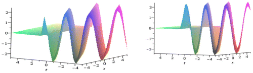
In this section, we have discussed about the obtained solution of the Kundu–Eckhaus equation and the derivative nonlinear Schrodinger equation. Using the MSE method, we get the traveling wave solutions from Equations (3.16) to (3.24) and Equations (3.39) to (3.45), respectively. From the above solution, it has been detected that the solutions represent the periodic solutions. These solutions are general closed form traveling wave solutions which are all periodic bell shape but different in amplitude. The solutions (3.19), (3.22), and (3.24) are in complex form. Therefore, the modulus and arguments of these solutions have been plotted. The graph of modulus and arguments of the solution (3.19) for α = β = 1, δ = 2, σ = 3 within $-10\le x,t\ge -10$ have been shown in Figure 1 and the graph of modulus and arguments of the solution (3.22) for α = δ = 1, β = −2, σ = 3 within $-5\le x,t\ge -5$ have been shown in Figure 2.

Figure 1. Plot of the modulus and arguments of the solutions u(x, t) in (3.19) to the Kundu–Eckhaus equation.

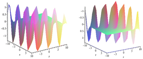
Figure 2. Plot of the modulus and arguments of the solutions u(x, t) in (3.22) to the Kundu–Eckhaus equation.

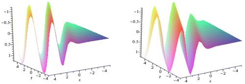
From the solutions of the derivative nonlinear Schrodinger equation, it is observed that α ≠ 1 ≠ β. The solutions (3.39) to (3.45) are traveling wave solutions which are all periodic bell shape in different amplitude. The solutions (3.42) and (3.45) are in complex form. Therefore, the modulus and arguments of these solutions have been plotted. The graph of modulus and arguments of that solution of (3.42) for α = 2, β = 1 within $-5\le x,t\ge -5$ have been shown in Figure 3.

Figure 3. Plot of the modulus and arguments of the solutions u(x, t) in (3.42) to nonlinear Schrodinger equation.

4.1. Remarks

The solutions are verified to check the correctness of the solutions by putting them back into the original equation and found correct.

5. Conclusion

In this article, the modified simple equation method has been successfully used to find the exact traveling wave solutions of Kundu–Eckhaus equation and derivative nonlinear Schrodinger equation. We obtain abundant closed form solutions of the aforesaid wave equations will be useful to analyze wave pattern in nonlinear optics, plasma physics, fluid mechanics, magneto-hydrodynamic wave equations. It is important to point out that the modified simple equation method is direct, concise, elementary, and comparing to other methods, like tanh–coth method, Jacobi elliptic function method, Exp-function method. The coefficients, $a_0,a_1$, etc. are attained without using any symbolic computation software such as Maple, Mathematica, etc. This method is easier, straightforward, and effective to handling. Therefore, the method can be used in further works to obtain exact solutions of other NLEEs in mathematical physics and engineering fields.

Additional information

Funding

Funding. The authors received no direct funding for this research.

Notes on contributors

A.K.M. Kazi Sazzad Hossain

A.K.M. Kazi Sazzad Hossain is an assistant professor at the Department of Mathematics, Begum Rokeya University, Rangpur, Bangladesh. Earlier in 2012, he joined at the same Department as a lecturer. He obtained his BSc (Honors) degree from the Department of Mathematics and MSc degree from the Department of Applied Mathematics, University of Rajshahi, Bangladesh. At present he is undertaking PhD at the Department of Applied Mathematics, University of Rajshahi, Bangladesh. He has published three research article and submitter another four.

M. Ali Akbar

M. Ali Akbar is an associate professor at the Department of Applied Mathematics, University of Rajshahi, Bangladesh. He received his PhD in Mathematics from the Department of Mathematics, University of Rajshahi, Bangladesh. He is actively involved in research in the field of nonlinear differential equations and fractional calculus. He has published more than 150 research articles of which 60 articles are published in ISI (Thomson Reuter) indexed journals and other 15 articles published in Scopus indexed journals.

References

- Abdou, M. A. (2007). The extended tanh-method and its applications for solving nonlinear physical models. Applied Mathematics and Computation, 190, 988–996.10.1016/j.amc.2007.01.070
- Adomian, G. (1994). Solving frontier problems of physics: The decomposition method. Boston, MA: Kluwer Academic.10.1007/978-94-015-8289-6
- Akbar, M. A., & Ali, N. H. M. (2011). Exp-function method for Duffing equation and new solutions of (2+1) dimensional dispersive long wave equations. Progress in Applied Mathematics, 1, 30–42.
- Akbar, M. A., Ali, N. H. M., & Mohyud-Din, S. T. (2012). The alternative (G′/G)-expansion method with generalized Riccati equation: Application to fifth order (1+1)-dimensional Caudrey-Dodd-Gibbon equation. International Journal of Physical Sciences, 7, 743–752.
- Akbar, M. A., Ali, N. H. M., & Zayed, E. M. E. (2012). Abundant exact traveling wave solutions of the generalized Bretherton equation via (G′/G)-expansion method. Communications in Theoretical Physics, 57, 173–178.10.1088/0253-6102/57/2/01
- Akter, J., & Ali Akbar, M. (2015). Exact solutions to the Benney-Luke equation and the Phi-4 equations by using modified simple equation method. Results in Physics, 5, 125–130.10.1016/j.rinp.2015.01.008
- Alam, M. N., Akbar, M. A., & Roshid, H. O. (2013). Study of nonlinear evolution equations to construct traveling wave solutions via the new approach of generalized (G′/G) -expansion method. Math. Stat., 1, 102–112.
- Bekir, A., & Boz, A. (2008). Exact solutions for nonlinear evolution equations using Exp-function method. Physics Letters A, 372, 1619–1625.10.1016/j.physleta.2007.10.018
- Biswas, A., & Porsezian, K. (2007). Soliton perturbation theory for the modified nonlinear Schrödinger’s equation. Communications in Nonlinear Science and Numerical Simulation, 12, 886–903.10.1016/j.cnsns.2005.11.006
- Biswas, A., Zony, C., & Zerrad, E. (2008). Soliton perturbation theory for the quadratic nonlinear Klein-Gordon equation. Applied Mathematics and Computation, 203, 153–156.
- Çevikel, A. C., Bekir, A., Akar, M., & San, S. (2012). A procedure to construct exact solutions of nonlinear evolution equations. Pramana, 79, 337–344.10.1007/s12043-012-0326-1
- Champeaux, S., Laveder, D., Passot, T., & Sulem, P-L. (1999). Remarks on the parallel propagation of small-amplitude dispersive Alfvénic waves. Nonlinear Processes in Geophysics, 6, 169–178.10.5194/npg-6-169-1999
- Chen, Y., & Wang, Q. (2005). Extended Jacobi elliptic function rational expansion method and abundant families of Jacobi elliptic function solutions to (1+1)-dimensional dispersive long wave equation. Chaos, Solitons & Fractals, 24, 745–757.10.1016/j.chaos.2004.09.014
- Chow, K. W. (1995). A class of exact, periodic solutions of nonlinear envelope equations. Journal of Mathematical Physics, 36, 4125–4137.10.1063/1.530951
- Fan, E. G. (2000). Extended tanh-function method and its applications to nonlinear equations. Physics Letters A, 277, 212–218.10.1016/S0375-9601(00)00725-8
- Guo, A. L., & Lin, J. (2010). Exact solutions of (2+1)-dimensional HNLS equation. Communications in Theoretical Physics, 54, 401–406.
- He, J. H. (2008). An elementary introduction to recently developed asymptotic methods and nanomechanics in textile engineering. International Journal of Modern Physics B, 22, 3487–3578.10.1142/S0217979208048668
- He, Y., Li, S., & Long, Y. (2012). Exact solutions of the Klein-Gordon equation by modified Exp-function method. Int. Math. Forum, 7, 175–182.
- Hirota, R. (1973). Exact envelope soliton solutions of a nonlinear wave equation. Journal of Mathematical Physics, 14, 805–809.10.1063/1.1666399
- Hirota, R., & Satsuma, J. (1981). Soliton solutions of a coupled KDV equation. Physics Letters A, 85, 404–408.
- Islam, R., Alam, M. N., Sazzad Hossain, A. K. M. K., Roshid, H. O., & Akbar, M. A. (2013). Traveling wave solutions of nonlinear evolution equations via Exp(−Φ(η))-expansion method. Global Journal of Science Frontier, 13, 63–71.
- Jawad, A. J. M., Petković, M. D., & Biswas, A. (2010). Modified simple equation method for nonlinear evolution equations. Applied Mathematics and Computation, 217, 869–877.10.1016/j.amc.2010.06.030
- Khan, K., & Akbar, M. A. (2013a). Application of exp(−Φ(η))-expansion method to find the exact solutions of modified Benjamin-Bona-Mahony equation. World Applied Sciences Journal, 24, 1373–1377.
- Khan, K., & Akbar, M. A. (2013b). Exact and solitary wave solutions for the Tzitzeica-Dodd-Bullough and the modified KdV-Zakharov-Kuznetsov equations using the modified simple equation method. Ain Shams Engineering Journal, 4, 903–909.10.1016/j.asej.2013.01.010
- Khan, K., Akbar, M. A., & Ali, N. H. M. (2013). The modified simple equation method for exact and solitary wave solutions of nonlinear evolution equation: The GZK-BBM equation and right-handed non-commutative burgers equations. ISRN Mathematical Physics, 5 pp. doi:10.1155/2013/146704
- Levko, D., & Volkov, A. (2006). Modeling of Kundu–Eckhaus equation. ArXiv: nlin.PS/0702050.
- Liu, S., Fu, Z., Liu, S. D., & Zhao, Q. (2001). Jacobi elliptic function expansion method and periodic wave solutions of nonlinear wave equations. Physics Letters A, 289, 69–74.10.1016/S0375-9601(01)00580-1
- Manafianheris, J. (2012). Exact Solutions of the BBM and MBBM Equations by the Generalized (G'/G )-expansion Method Equations. International Journal of Genetic Engineering, 2(3), 28–32.10.5923/j.ijge.20120203.02
- Naher, H., Abdullah, A. F., & Akbar, M. A. (2011). The Exp-function method for new exact solutions of the nonlinear partial differential equations. International Journal of Physical Sciences, 6(29), 6706–6716.
- Naher, H., Abdullah, A. F., & Akbar, M. A. (2012). New traveling wave solutions of the higher dimensional nonlinear partial differential equation by the Exp-function method. Journal of Applied Mathematics, 2012, Article ID: 575387, 14 pp.
- Nassar, H. A., Abdel-Razek, M. A., & Seddeek, A. K. (2011). Expanding the tanh-function method for solving nonlinear equations. Applied Mathematics, 2, 1096–1104.
- Neyrame, A., Roozi, A., Hosseini, S. S., & Shafiof, S. M. (2010). Exact travelling wave solutions for some nonlinear partial differential equations. Journal of King Saud University - Science, 22, 275–278.10.1016/j.jksus.2010.06.015
- Sirendaoreji. (2004). New exact travelling wave solutions for the Kawahara and modified Kawahara equations. Chaos, Solitons & Fractals, 19, 147–150.10.1016/S0960-0779(03)00102-4
- Taghizadeh, N., & Mirzazadeh, M. (2011). The first integral method to some complex nonlinear partial differential equations. Journal of Computational and Applied Mathematics, 235, 4871–4877.10.1016/j.cam.2011.02.021
- Wang, M. (1995). Solitary wave solutions for variant Boussinesq equations. Physics Letters A, 199, 169–172.10.1016/0375-9601(95)00092-H
- Wang, M. L., & Zhou, Y. B. (2003). The periodic wave solutions for the Klein–Gordon–Schrödinger equations. Physics Letters A, 318, 84–92.10.1016/j.physleta.2003.07.026
- Wazwaz, A. M. (2004). A sine-cosine method for handlingnonlinear wave equations. Mathematical and Computer Modelling, 40, 499–508.10.1016/j.mcm.2003.12.010
- Weiss, J., Tabor, M., & Carnevale, G. (1982). The Painlevé property for partial differential equations. Journal of Mathematical Physics, 24, 522–526.
- Yan, Z., & Zhang, H. (2001). New explicit solitary wave solutions and periodic wave solutions for Whitham Broer-Kaup equation in shallow water. Physics Letters A, 285, 355–362.10.1016/S0375-9601(01)00376-0
- Yang, L., Liu, J., & Yang, K. (2001). Exact solutions of nonlinear PDE, nonlinear transformations and reduction of nonlinear PDE to a quadrature. Physics Letters A, 278, 267–270.10.1016/S0375-9601(00)00778-7
- Zayed, E. M. E., & Ibrahim, S. A. H. (2012). Exact solutions of nonlinear evolution equations in mathematical physics using the modified simple equation method. Chinese Physics Letters, 29, 060201.10.1088/0256-307X/29/6/060201
- Zayed, E. M. E., & Shorog, A. J. (2013). Applications of an extended (G′/G)-expansion method to find exact solutions of nonlinear PDEs in Mathematical Physics. Mathematical Problems in Engineering, Article ID: 768573, 19 pp. doi:10.1155/2010/768573
- Zayed, E. M. E., Zedan, H. A., & Gepreel, K. A. (2004). On the solitary wave solutions for nonlinear Hirota–Satsuma coupled KdV of equations. Chaos, Solitons & Fractals, 22, 285–303.10.1016/j.chaos.2003.12.045
- Zhang, J., Jiang, F., & Zhao, X. (2010). An improved (G′/G)-expansion method for solving nonlinear evolution equations. International Journal of Computer Mathematics, 87, 1716–1725.10.1080/00207160802450166