Savings operations over random periods

Abstract

Due to the ageing of the population, public pension plans are increasingly being implemented by private savings schemes. This therefore gives rise to a wide range of innovative schemes to meet the varying needs of savers and financial institutions. Therefore, the aim of this paper is to propose a savings operation which includes the randomness derived from the contingency which supposes the eventual but unpredictable death of the saver. We have developed this type of operation by applying a financial-actuarial methodology and thereby deducing a way of calculating all amounts resulting from the savings operation, and introducing a new quantity derived from this randomness, namely the risk quota. Similarly, we have indicated how to calculate different measures of (gross and net) profitability, in random terms and the part corresponding to this randomness.

Keywords:

• pension plans
• savings operations
• profitability
• savings quota
• risk quota
• probability of survival

JEL Classification:

• G22
• G23
• H55

Public interest statement

The increase in life expectancy and consequent increase in the number of people of pensionable age, accompanied by a reduction in the birth rate, have given rise to a greater ratio of pensioners to workers. This supposes a problem for the maintenance of the system of public pensions in the majority of developed countries. Population must be aware that they have to contract private savings plans in order to complement their incomes when they become retired. Therefore, it is necessary to develop savings products which are attractive to the saver and adapted to their particular family situation and their attitude to risk, by encouraging citizens to have their own private savings plans. Consequently, this manuscript proposes two different savings products which incorporate the risk derived from the investor’s survival to traditional savings operations and shows how to determine the different magnitudes involved in such operations.

1. Justification of the research

The increase in life expectancy and consequent increase in the number of people of pensionable age, accompanied by a reduction in the birth rate, have given rise to a greater proportion of pensioners to workers. This supposes a problem for the maintenance of public pensions in many of the advanced countries (Fong, Piggott, & Sherris, 2015; Komp & Johansson, 2016; Martin, 2011). According to the projections estimated by the European Commission, public expenditure in pensions within the European Union is estimated to reach 12.9% of the GDP in 2060. Spain, together with Belgium, Denmark, Ireland, Greece, Luxembourg, Austria and Portugal, is one of the countries which will reach a higher percentage of its GDP dedicated to pensions, estimated at 13.7% (EU-COMMISSION, 2012).

Consequently, it is necessary to introduce some changes in the current pension models, based on the system of distribution (the contributions of present-day workers serve to pay the pensions of those now in retirement) in order to guarantee its future viability (Balsameda, Melguizo, & Taguas, 2006; Ni & Podqursky, 2016). In effect, in order to reduce the cost of public pension plans, some governments such as the USA (Clark, Hanson, & Mitchell, 2016; Farrell & Shoag, 2016; Lewis & Stoycheva, 2016; Platanakis & Sutcliffe, 2016) and United Kingdom (Danzer, Dolton, & Bondibene, 2016; Disney, 2016) have already begun to take some measures.

There are two ways of implementing the necessary changes. On the one hand, some parametric reforms consisting of certain adjustments may be devised without changing substantially the original model, such reforms imply a reduction of pensions and/or an increase in workers contributions (Boldrin, Dolado, Jimeno, & Peracchi, 1999; Hammond et al., 2016; Yang, 2016). On the other hand, the changes can consist of moving towards the so-called models of individual capitalization, similar to private plans, or towards mixed systems, where a minimal pension will be guaranteed and complemented with voluntary private pensions (Cesaratto, 2002, 2006; Febrero & Cadarso, 2006; Wang, Williamson, & Cansoy, 2016); in the latter case, fiscal incentives are applied to the quotas contributed to private systems.

Private saving for retirement, as demonstrated by several empirical works, is related to social and demographic aspects, such as age (Fernández, Vivel, Motero, & Rodeiro, 2012; Hira, Rock, & Loibl, 2009; Huberman, Iyengar, & Jiang, 2007), educational level (Seong-Lim, Myung-Hee, & Montalto, 2000), area of residence (Fontes, 2011; Harris, Loundes, & Webster, 2002) or belonging to certain groups, such as immigrants (Harrysson, Montesino, & Werner, 2016), among others.

It can be stated that the risk of longevity, that is to say, the probability of exceeding the period covered by retirement savings, is an important economic risk, whereby it is necessary to foresee the income of people in this situation. It must be borne in mind that nowadays, a person can survive for more than 30 years in a retirement situation (Forman, 2016). Consequently, it becomes necessary to introduce some financial products adjusted to the needs of savers because innovation in this field is essential to satisfy these. Our aim is to put at the disposal of savers who make private provision for retirement a financial savings product adjusted to the contingency determined by their own life expectancy.

In traditional savings operations, both the commencement and the end of the savings period are known; that is to say, these instants are well-known a priori. An analogous characteristic is exhibited by the withdrawal of the accumulated amount (Valls Martínez & Cruz Rambaud, 2013). However, some savings operations can be agreed by assuming that the commencement or the end of periodic deposits is random, depending on a contingency; moreover, this randomness could also affect the final withdrawal if the two parts of the operation agree. Here, we consider a savings operation in which deposits have a fixed commencement but the end is unknown (random). In other words, although the deposits commence and terminate at times agreed on formalizing the operation, the actual duration of the period of deposits is linked to the survival of saver in such a way that the deposits finish on premature death. In these circumstances, we can distinguish two possible cases:

1. If the investor dies before the date of the final withdrawal, that is to say, during the expected duration of the savings period, the operation finishes, and consequently both the right to receive the final amount by the saver and his obligation to make the rest of the periodic deposits will disappear. As a consequence, all deposited money up to that moment will stay in favour of the financial institution, because its obligation to return the deposits plus the corresponding interest vanishes.

2. If the investor dies before the date of the final withdrawal, the periodic deposits will cease, but the person designated by him will receive the final agreed amount as if the operation had not suffered any contingency, that is to say, as if the periodic deposits had continued during the entire initially agreed period. In such a case, the final agreed amount will be received by the beneficiary.

This paper is structured as follows. In Section 2, we present the new proposed savings operation from a financial point of view, by specifying the different possibilities which can arise and their respective treatment. In Section 3, we describe in detail the different quantities which define the savings operation when the withdrawal of the amount depends on the survival of the investor, as well as the different measures of profitability which arise when considering randomness. Analogously, Section 4 considers the case in which the withdrawal of the amount is fixed. Finally, Section 5 summarizes and concludes.

It is worth noting to indicate that, for the sake of brevity, the mathematical developments leading to the expressions of the different amounts in Sections 2–4 are not be detailed. Instead, in each case, we indicate only the starting point of the reasoning and the final expression.

2. General financial approach to a savings operation with random terminal date

Let us consider a savings operation consisting of the periodic deposit by the investor of n amounts $a_s$, where $s=1,2,\dots ,n$, with maturity at instant $s-1$, respectively, with the aim to reach a final amount $C_m$ at instant m, being $m\le n$. In traditional savings operations, where randomness is not considered, the equation of financial equivalence at the commencement of the operation, by using the exponential discounting at a variable interest rate i_s for each period, is (Valls Martínez & Cruz Rambaud, 2014)

(1) $C_m\cdot \prod _{h=1}^m(1+i_h{)}^{-1}=\sum _{s=1}^n{a}_s\cdot \prod _{h=1}^{s-1}(1+i_h{)}^{-1},$(1)

However, if the periodic deposits and the withdrawal of the final amount are subject to a certain contingency, the equation of random, financial equivalence will be

(2) $C_m\cdot \prod _{h=1}^m(1+i_h{)}^{-1}\cdot (1+r_h{)}^{-1}=\sum _{s=1}^n{a}_s\cdot \prod _{h=1}^{s-1}(1+i_h{)}^{-1}\cdot (1+r_h{)}^{-1},$(2)

where $r_h$ denotes the variable interest rate corresponding to period h.

Where the contingency is the death of the saver, the risk measured by $r_h$ is the probability that the saver dies and, consequently, the probability that both his right to receive the final amount and his obligation to make periodic deposits disappear. Therefore, by considering the saver’s survival, one has

(3) $1+r_h=\frac{1}{{ }_1{p}_{h-1}},$(3)

where ${\hspace{0.17em}}_1^{\hspace{0.17em}}{p}_{h-1}$ is the probability that a person aged $h-1$ reaches the age h, being

(4) ${\hspace{0.17em}}_1^{\hspace{0.17em}}{p}_{h-1}=\frac{l_h}{l_{h-1}}$(4)

and $l_h$ is the number of persons reaching age h.

Equations (2) and (3) lead to

(5) $C_m\cdot \prod _{h=1}^m(1+i_h{)}^{-1}\cdot {\hspace{0.17em}}_1^{\hspace{0.17em}}{p}_{h-1}=\sum _{s=1}^n{a}_s\cdot \prod _{h=1}^{s-1}(1+i_h{)}^{-1}\cdot {\hspace{0.17em}}_1^{\hspace{0.17em}}{p}_{h-1},$(5)

where $\frac{l_s}{l_0}=p_s$ is the probability of survival at instant s. Thus,

(6) $C_m\cdot p_m\cdot \prod _{h=1}^m(1+i_h{)}^{-1}=\sum _{s=1}^n{a}_s\cdot p_{s-1}\cdot \prod _{h=1}^{s-1}(1+i_h{)}^{-1}$(6)

Equation (6) coincides with $C_n\cdot {\hspace{0.17em}}_n^{\hspace{0.17em}}{E}_x=\sum _{s=1}^n{a}_s\cdot {\hspace{0.17em}}_{s-1}^{\hspace{0.17em}}{E}_x$ (Valls Martínez & Cruz Rambaud, 2016), where ${\hspace{0.17em}}_s^{\hspace{0.17em}}{E}_x={\hspace{0.17em}}_s^{\hspace{0.17em}}{p}_x\cdot \prod _{h=1}^s(1+i_h{)}^{-1}$ is the factor of actuarial discounting.

Observe that, in expression (6), the subscript s refers to the instant at which the corresponding scheme matures. Therefore, $l_0$ is the number of living persons belonging to the saver’s generation at the commencement of the savings operation. Thus, for example, if the investor is 50 at the commencement of the operation, $l_0$ is the number of persons of this generation who remain alive at this age. Analogously, $l_{10}$ is the number of persons of this generation who have reached the age of 60 years, in such a way that $p_{10}$ is the probability of a person aged 50 to reach 60. According to the notation by Valls Martínez and Cruz Rambaud (2016), this is the same as ${ }_{10}^{\hspace{0.17em}}{p}_{50}$.

If we denote:

(7) $a{}_s^{\prime }:=\frac{a_s}{p_m},$(7)

from Equation (6), we can deduce that

(8) $C_m\cdot \prod _{h=1}^m(1+i_h{)}^{-1}=\sum _{s=1}^{n}a{}_s^{\prime }\cdot p_{s-1}\cdot \prod _{h=1}^{s-1}(1+i_h{)}^{-1},$(8)

which indicates that, with the deposit of amounts $a{}_s^{\prime }$, the saver (in the case of survival) or his beneficiaries (in the case of the investor’s death) will receive the amount $C_m$ at instant m. Observe that $a{}_s^{\prime }>a_s$, which is logical since, with the deposit of $a{}_s^{\prime }$, the withdrawal of the final amount will be sure, whilst with the deposit of $a_s$, this amount is not guaranteed.

On the other hand, by considering

(9) $a{}_s^{\prime \prime }:=a{}_s^{\prime }\cdot p_{s-1}=a_s\cdot \frac{p_{s-1}}{p_m},$(9)

one has

(10) $C_m\cdot \prod _{h=1}^m(1+i_h{)}^{-1}=\sum _{s=1}^{n}a{}_s^{\prime \prime }\cdot \prod _{h=1}^{s-1}(1+i_h{)}^{-1},$(10)

the equation which indicates the financial equivalence between the fixed deposits and the total withdrawal. It is obvious that

(11) $a_s<a{}_s^{\prime \prime }<a{}_s^{\prime },$(11)

because $a{}_s^{\prime }$ and $a{}_s^{\prime \prime }$ must guarantee the sure withdrawal of the final amount $C_m$ and, moreover, $a{}_s^{\prime }$ has to compensate the randomness of the periodic deposits.

Therefore, the periodic deposits to save $C_m$ at instant m are

• $a_s$, in the case of the probable survival of the saver, which guarantees neither the future periodic deposits nor the final withdrawal.

• $a{}_s^{\prime }:=\frac{a_s}{p_m}$, in the case of the withdrawal of $C_m$ being guaranteed, but not the periodic deposits, which depend on the investor’s survival.

• $a{}_s^{\prime \prime }:=a_s\cdot \frac{p_{s-1}}{p_m},$ in the case of both the withdrawal of $C_m$ and the periodic deposits being guaranteed.

Thus, we can state that in the case of deposit $a{}_s^{\prime }$, for every s, the final saved amount should be

• $C_m$, in the case of withdrawal only if the investor survives at instant m,

• $C{}_m^{\prime }$, in the case of the withdrawal of an agreed amount by the investor (if he survives) or by his beneficiaries (if he dies), and the relationship between these amounts is

  $C{}_m^{\prime }=C_m\cdot p_m,$

where logically, $C{}_m^{\prime }<C_m$.

Table 1 presents a summary of the possible situations to reach the final amount $C_m$.

Table 1. Randomness and discount factor

Periodic deposits	$a_s$	$a{}_s^{\prime }$	$a{}_s^{\prime \prime }$
Randomness of deposits	Yes	Yes	No
Randomness of the final amount	Yes	No	No
Discounting of deposits	Actuarial	Actuarial	Exponential
Discounting of the final amount	Actuarial	Exponential	Exponential

Hereinafter, we will assume that $m=n$, that is to say, once the saver has received the final total amount, the periodic deposits finish since logically from this moment, the savings period has expired and there is no reason to continue with the deposits.

3. The withdrawal of the final amount depends on the investor’s survival

In this case, as previously indicated, the financial equivalence at time 0 is given by the following equation:

(12) $C_n\cdot p_n\cdot \prod _{h=1}^n(1+i_h{)}^{-1}=\sum _{s=1}^n{a}_s\cdot p_{s-1}\cdot \prod _{h=1}^{s-1}(1+i_h{)}^{-1}$(12)

The balance at an intermediate instant k, when both the deposits and the withdrawal of the final amount are random, by the retrospective method (according to the amounts between the commencement and instant k) is

(13) $C{}_k^{-}=\sum _{s=1}^k{a}_s\cdot \prod _{h=s}^k(1+i_h)\cdot (1+r_h)$(13)

which leads to

(14) $C_k^{-}=\frac{1}{p_k}\cdot \sum _{s=1}^k{a}_s\cdot p_{s-1}\cdot \prod _{h=s}^k(1+i_h)$(14)

Observe that, due to their randomness, both the deposits and the final amount are multiplied by an actuarial discount factor, as described in Table 1.

Likewise, the balance can be calculated by using the so-called prospective method (according to the amounts deposited between instant k and the end of the operation). To do this, we start from Equation (13) where simple algebra and some suitable simplifications result in

(15) $C{}_k^{-}=\frac{1}{p_k}\cdot \left[C_n\cdot p_n\cdot \prod _{h=k+1}^n{(1+i_h)}^{-1}-\left(\sum _{s=k+2}^n{a}_s\cdot p_{s-1}\cdot \prod _{h=k+1}^{s-1}{(1+i_h)}^{-1}\right)\right]-a_{k+1}$(15)

Finally, we can also obtain the balance by the recurrent method, according to the balance obtained in the former period. In this way, starting from Equation (15) and following an adequate process, one has

(16) $C{}_{k+1}^{-}=(C{}_k^{-}+a_{k+1})\cdot (1+i_{k+1})\cdot \frac{p_k}{p_{k+1}}$(16)

The partial balance in a given period k, denoted by ${\mathrm{\Delta }}_k^{-}$, is the difference between the balance at the end, $C{}_k^{-}$, and at the beginning, $C{}_{k-1}^{-}$, of said period:

${\mathrm{\Delta }}_k^{-}:=C{}_k^{-}-C{}_{k-1}^{-},$

which, by considering Equation (16) and simple algebra, leads to

(17) ${\mathrm{\Delta }}_k^{-}=(C{}_{k-1}^{-}+a_k)\cdot \frac{p_{k-1}}{p_k}\cdot i_k+C{}_{k-1}^{-}\cdot \left(\frac{p_{k-1}}{p_k}-1\right)+a_k\cdot \frac{p_{k-1}}{p_k},$(17)

where the interest quota corresponding to period k, denoted by $I_k$, is

(18) $I_k:=(C{}_{k-1}^{-}+a_k)\cdot \frac{p_{k-1}}{p_k}\cdot i_k$(18)

and the savings quota, denoted by $q_k$, is

(19) $q_k:=C{}_{k-1}^{-}\cdot \left(\frac{p_{k-1}}{p_k}-1\right)+a_k\cdot \frac{p_{k-1}}{p_k}$(19)

Observe that $q_k$ is the amount which, together with the interests, increases the balance accrued at the end of a former period to obtain the current balance.

In general, in the savings operations with an element of risk, the deposits made by the saver (say $a_s$) do not coincide with the amounts which generates the saving (viz $q_s$). The difference between them is called the risk quota, denoted by $g_s$. Thus, for a given period k

(20) $g_k:=a_k-q_k$(20)

In this case, there is a risk associated with the periodic deposits because they finish if the saver dies. But the final amount is also affected by this risk, because if the investor dies, he loses the entire saved amount. In order to compensate this risk, the saver will receive a bigger final amount in the event of survival at the end of the agreed period. This makes the risk quota negative, by indicating the “surplus” obtained by the investor for assuming this risk.

Definitively, by considering Equations (19) and (20) and applying simple algebra, this gives

(21) $g_k=(a_k+C{}_{k-1}^{-})\cdot \left(1-\frac{p_{k-1}}{p_k}\right)$(21)

Observe that, as $p_{k-1}>p_k$, one has $g_k<0$. Observe also that, as ${\mathrm{\Delta }}_k^{-}=I_k+q_k$, one has $q_k={\mathrm{\Delta }}_k^{-}-I_k$ and then

$g_k=a_k+I_k-{\mathrm{\Delta }}_k^{-},$

which, obviously, is less than 0.

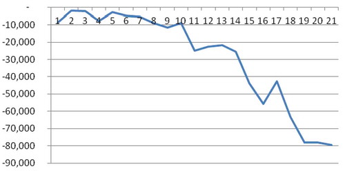
Example 1. Assume that, in 2013, a person aged 50 wishes to save an amount of 10,000 Euros during a period of 21 years, that is to say, to be withdrawn at age 71, if he survives. If he does not, the deposits will remain in the possession of the account’s promoter. If the agreed effective yearly interest rate is 3%, the deposits should be of 314.25 Euros. The different quantities corresponding to this random savings operation appear in Table 2.

Table 2. Savings operation when the withdrawal of the final amount depends on the investor's survival

Year	I	As	Ps	gs	qs	Is	${\mathbf{\Delta }}_{\mathit{s}}^{\mathbf{-}}$	$\mathit{C}{}_s^{-}$	${\mathit{M}}_s^{-}$
0	−	−	1	−	−	−	−	−	10,000.00
1	0.03	314.25	0.973	–8.72	322.97	9.69	332.66	332.66	9,667.34
2	0.03	314.25	0.970	–1.85	316.10	19.46	335.56	668.22	9,331.78
3	0.03	314.25	0.968	–2.21	316.46	29.54	346.00	1,014.22	8,985.78
4	0.03	314.25	0.962	–7.73	321.98	40.09	362.06	1,376.28	8,623.72
5	0.03	314.25	0.961	–2.94	317.19	50.80	368.00	1,744.28	8,255.72
6	0.03	314.25	0.958	–5.04	319.29	61.91	381.20	2,125.47	7,874.53
7	0.03	314.25	0.956	–5.46	319.71	73.36	393.07	2,518.54	7,481.46
8	0.03	314.25	0.953	–9.10	323.35	85.26	408.60	2,927.14	7,072.86
9	0.03	314.25	0.950	–11.47	325.72	97.59	423.31	3,350.45	6,649.55
10	0.03	314.25	0.948	–9.04	323.29	110.21	433.50	3,783.95	6,216.05
11	0.03	314.25	0.942	–25.02	339.26	123.70	462.96	4,246.92	5,753.08
12	0.03	314.25	0.937	–22.74	336.99	137.52	474.51	4,721.43	5,278.57
13	0.03	314.25	0.933	–21.69	335.94	151.72	487.66	5,209.09	4,790.91
14	0.03	314.25	0.929	–25.52	339.77	166.47	506.24	5,715.32	4,284.68
15	0.03	314.25	0.922	–43.66	357.91	182.20	540.11	6,255.43	3,744.57
16	0.03	314.25	0.914	–55.59	369.84	198.76	568.60	6,824.02	3,175.98
17	0.03	314.25	0.909	–42.70	356.95	215.43	572.38	7,396.41	2,603.59
18	0.03	314.25	0.902	–63.28	377.53	233.22	610.75	8,007.15	1,992.85
19	0.03	314.25	0.893	–77.93	392.18	251.98	644.16	8,651.31	1,348.69
20	0.03	314.25	0.885	–78.13	392.38	271.31	663.69	9,315.00	685.00
21	0.03	314.25	0.878	–79.49	393.74	291.26	685.00	10,000.00	−
Total		6,599.24	−	–599.31	7,198.54	2,801.46	10,000.00	−	−

The last column in Table 2, $M_s^{-}$ represents the pending amount to be saved, which is the difference between the final amount and the balance, that is to say, $C{}_n-C{}_s^{-}$.

Figure 1 shows that, in effect, the risk quota is negative. Moreover, despite the fact that it varies throughout the operation, it exhibits a pronounced decreasing tendency as the investor’s age increases. As indicated, this quota compensates the increasing risk of losing the saved amount due to the possible death of the investor.

Figure 1. Risk quota when the withdrawal of the final amount depends on the investor's survival

If the details of the operation are fixed, that is to say, if regular deposits of 314.25 Euros are made to save a fixed amount during the period of 21 years, then the final amount will be 9,281.92 Euros. In this case, it will be necessary to make 23 deposits to save 10,000 Euros. In effect, the number of necessary deposits is given by the following equation:

$10,000=314.25\cdot 1.03\cdot \frac{{1.03}^n-1}{0.03},$

from where n = 22.19 years.

Obviously, these savings operations can also be designed by using a variable interest rate. In such a case, it is necessary to calculate the average interest rate, denoted by $i_m$, derived from the total contract period. This rate, applied to all periods of the operation, establishes the financial equivalence between the deposits and the final amount. Thus, given the values of $C{}_n$, $a_s$ and $p_s$, the average interest rate can be calculated by using the following equation:

(22) $C_n\cdot p_n\cdot (1+i_m{)}^{-n}=\sum _{s=1}^n{a}_s\cdot p_{s-1}\cdot (1+i_m{)}^{-(s-1)}$(22)

It is necessary to point out that, if the operation finishes at an instant $k<n$ due to the investor’s death, it does not make sense to talk about the profitability for the investor or the cost for the administrator. One must refer to the loss or benefit, respectively, equal to the deposits accumulated up to the time of death.

When initially agreed, the duration of this type of operation (and its termination) is not known. Nevertheless, its distribution of probability is well known, which allows us to calculate the average estimated duration, denoted by $\bar{k}$, and will be the expected conclusion of the operation.

The probability of each duration k, denoted by ${\hspace{0.17em}}_1^{\hspace{0.17em}}{f}_k$, for $k=1,2,\dots ,n-1$, is given by the probability of death between the ages $k-1$ and $k$:

${\hspace{0.17em}}_1^{\hspace{0.17em}}{f}_{k-1}=p_{k-1}-p_k.$

For $k=n$, the probability of this duration is $p_{n-1}$, which is the probability that the investor dies at a later date. Therefore,

(23) $\bar{k}=E\left[k\right]=\sum _{k=1}^{n-1}k\cdot {\hspace{0.17em}}_1^{\hspace{0.17em}}{f}_{k-1}+n\cdot p_{n-1}$(23)

Finally, the financial completion of the random operation is the same as that of the fixed operation whose final amount coincides with that of the random operation, that is to say, the value $\tilde{k}$ satisfying the following equation:

(24) $C_n\cdot p_n\cdot \prod _{h=1}^n{(1+i_h)}^{-1}=\sum _{s=1}^n{a}_s\cdot p_{s-1}\cdot \prod _{h=1}^{s-1}{(1+i_h)}^{-1}=\sum _{s=1}^{\tilde{k}}{a}_s\cdot \prod _{h=1}^{s-1}{(1+i_h)}^{-1}$(24)

Equation (24) is very difficult to satisfy, that is to say, $\tilde{k}$ will not be an integer number, but instead, in most cases:

$\tilde{k}\in \left[\alpha ,\alpha +1\right[$, where $\alpha \in \mathrm{N}$,

being

$\sum _{s=1}^{\alpha }{a}_s\cdot \prod _{h=1}^{s-1}(1+i_h{)}^{-1}<C_n\cdot p_n\cdot \prod _{h=1}^n(1+i_h{)}^{-1}<\sum _{s=1}^{\alpha +1}{a}_s\cdot \prod _{h=1}^{s-1}(1+i_h{)}^{-1}.$

Example 2. Let us consider the data of Example 1 but assuming that the effective yearly interest rate will be 3% for the first 5 years and that after each 5-year period, the interest rate increases by 1%; thus, from year 6 to 10, the interest rate will be 4%, from year 11 to 15, 5%, from year 16 to 20, 6% and from year 21, 7%. In this case, the equation

$10,000\cdot 0.8782199\cdot (1+i_m{)}^{-21}=\sum _{s=1}^{21}242.27\cdot p_{s-1}\cdot (1+i_m{)}^{-(s-1)},$

gives 5.146601% as the average rate of the savings operation.

In this example, the estimated average duration at the beginning of the operation is 19.766 years, whereby the operation will finish when the saver is 69 (see Table 3).

Table 3. Average duration of the savings operation when the withdrawal of  the final amount depends on the investor's survival

Age	Year (k)	${ }_1{f}_{k-1}$	$k{\cdot }_1{f}_{k-1}$
50	1	0.02699721	0.026997205
51	2	0.00277555	0.005551108
52	3	0.00217587	0.006527624
53	4	0.00559711	0.022388456
54	5	0.00167278	0.008363881
55	6	0.00234749	0.014084937
56	7	0.00214105	0.014987385
57	8	0.00306079	0.024486286
58	9	0.00336134	0.030252092
59	10	0.00233786	0.023378563
60	11	0.00574866	0.063235249
61	12	0.00467283	0.056073972
62	13	0.00401907	0.052247874
63	14	0.00429169	0.060083655
64	15	0.00667691	0.100153673
65	16	0.00773699	0.123791811
66	17	0.00543752	0.092437842
67	18	0.00739907	0.133183186
68	19	0.00836459	0.158927173
69	20	0.00771624	0.154324867
70	21*	0.88546938	18.59485702
Average			19.7663339

*For $k=21$, the value of column ${\hspace{0.17em}}_1^{\hspace{0.17em}}{f}_{k-1}$ corresponds to $p=20$.

Finally, the financial conclusion of the operation lies in the interval [19,20[ since

$\sum _{s=1}^{19}{a}_s\cdot \prod _{h=1}^{s-1}(1+i_h{)}^{-1}=3,385.53<3,407.15<3,492.14=\sum _{s=1}^{20}{a}_s\cdot \prod _{h=1}^{s-1}(1+i_h{)}^{-1},$

being

$3,407.15=10,000.00\cdot 0.878219924140343\cdot {1.03}^{-5}\cdot {1.05}^{-5}\cdot {1.06}^{-5}\cdot {1.07}^{-1}.$

4. The withdrawal of the saved amount is at an agreed date

When the withdrawal of the saved amount is sure, either by the investor, in case of survival, or by his heirs, in the event of the investor’s death, the financial equivalence at the beginning of the savings operation is

(25) $C_n\cdot \prod _{h=1}^n(1+i_h{)}^{-1}=\sum _{s=1}^{n}a{}_s^{\prime }\cdot p_{s-1}\cdot \prod _{h=1}^{s-1}(1+i_h{)}^{-1}$(25)

Taking into account that the deposits are random and that the saved amount is fixed, the partial saved amount at a given intermediate instant k is not going to be conditioned by the survival probability at said instant. Thus, starting from Equation (14), the calculation by using the retrospective method results in

(26) $C{}_k^{-}=\sum _{s=1}^{k}a{}_s^{\prime }\cdot p_{s-1}\cdot \prod _{h=s}^k(1+i_h),$(26)

in accordance with Valls Martínez and Cruz Rambaud (2014):

$\prod _{h=1}^{\tau }(1+i_h{)}^{-1}\cdot V{\prime }_{\tau }^{-}=\sum _{s=1}^{\tau }{\mathrm{a}}_{\mathrm{s}}^{\prime }\cdot {}_{s-1}{E}_x$

Observe that, in this case, only the random deposits are multiplied by the actuarial discounting, whilst the saved amount, due to its lack of randomness, is multiplied by the exponential discounting, as indicated in Table 1.

Likewise, the balance can be calculated by using the so-called prospective method. To do this, we start from Equation (26) where simple algebra results in

(27) $C{}_k^{-}=C_n\cdot \prod _{h=k+1}^n(1+i_h{)}^{-1}-\left(\sum _{s=k+2}^n{a^{\prime }}_s\cdot p_{s-1}\cdot \prod _{h=k+1}^{s-1}{(1+i_h)}^{-1}+a{}_{k+1}^{\prime }\cdot p_k\right),$(27)

in accordance with Equation (15) since now the partial saved amount is not conditioned by the investor’s survival at said instant.

Finally, we can also obtain the balance by the recurrent method. In this way, starting from Equation (26) and doing some suitable simplifications, one has

(28) $C{}_{k+1}^{-}=(C{}_k^{-}+a{}_{k+1}^{\prime }\cdot p_k)\cdot (1+i_{k+1}).$(28)

The partial balance in a given period k, denoted by ${\mathrm{\Delta }}_k^{-}$, is the difference between the balance at the end, $C{}_k^{-}$, and at the beginning, $C{}_{k-1}^{-}$, of said period:

${\mathrm{\Delta }}_k^{-}:=C{}_k^{-}-C{}_{k-1}^{-},$

which, by considering Equation (28), leads to

(29) ${\mathrm{\Delta }}_k^{-}=(C{}_{k-1}^{-}+a{}_k^{\prime }\cdot p_{k-1})\cdot (1+i_k)-C{}_{k-1}^{-},$(29)

where by

${\mathrm{\Delta }}_k^{-}=(C{}_{k-1}^{-}+a{}_k^{\prime }\cdot p_{k-1})\cdot i_k+a{}_k^{\prime }\cdot p_{k-1},$

where the interest quota corresponding to period k, denoted by $I_k$, is

(30) $I_k:=(C{}_{k-1}^{-}+a{}_k^{\prime }\cdot p_{k-1})\cdot i_k,$(30)

and the savings quota, denoted by $q_k$ (the amount which, together with the interest, increases the balance accrued at the end of a former period to obtain the current balance), is

(31) $q_k:=a{}_k^{\prime }\cdot p_{k-1}$(31)

Observe that, in this case, the savings quota coincides with the deposit corresponding to the fixed savings operation, i.e.:

(32) $q_k=a{}_k^{\prime \prime }$(32)

The risk quota is known to be the difference between the periodic deposit and the savings quota which, in this case, is positive (except for the first period in which it is 0 because there is no risk for the first deposit), to compensate the financial entity for the possibility (risk) that the investor dies before finishing the periodic deposits. Thus,

(33) $g_k:=a{}_k^{\prime }-q_k$(33)

By considering Equation (36),

(34) $g_k=a{}_k^{\prime }\cdot (1-p_{k-1}),$(34)

which, in effect, is not negative, that is, $g_k\ge 0$. Consequently, in this type of operation, if the investor lives beyond a given instant, he would save more than in a riskless operation, which moreover implies a profit for the financial entity which is greater than that obtained if deposits are made in the context of a savings operation of fixed duration (and vice versa).

In this case, the risk quota (see Equations (32) and (33)) is the difference between the deposit when the conclusion of the savings operation is random and the saved amount is fixed, and the deposit corresponding to a savings operation where both the deposits and the saved amount are fixed. That is to say:

(35) $g_k=a{}_k^{\prime }-a{}_k^{\prime \prime }$(35)

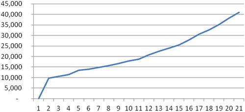
Example 3. Assume that, in 2013, a person aged 50 wishes to save an amount of 10,000 Euros over a period of 21 years, that is to say, to be withdrawn by him at age 71 if he survives, or by his heirs, in the event of the investor’s early death. If the agreed effective yearly interest rate is 3%, the periodic deposits should be of 314.25 Euros. The different quantities corresponding to this random savings operation appear in Table 4.

Table 4. Savings operation when the withdrawal of the saved amount is at an agreed date

Year	I	As	Ps	${\mathit{g}}_s$	$q_s$	Is	${\mathrm{\Delta }}_s^{-}$	$\mathit{C}{}_s^{-}$	${\mathit{M}}_s^{-}$
0	−	−	1	−	−	−	−	−	10,000,00
1	0.03	357.83	0.973	−	357.83	10.73	368.56	368.56	9,631,44
2	0.03	357.83	0.970	9.66	348.17	21.50	369.67	738.23	9,261,77
3	0.03	357.83	0.968	10.65	347.17	32.56	379.73	1,117.96	8,882,04
4	0.03	357.83	0.962	11.43	346.39	43.93	390.32	1,508.29	8,491,71
5	0.03	357.83	0.961	13.43	344.39	55.58	399.97	1,908.26	8,091,74
6	0.03	357.83	0.958	14.03	343.79	67.56	411.35	2,319.61	7,680,39
7	0.03	357.83	0.956	14.87	342.95	79.88	422.83	2,742.44	7,257,56
8	0.03	357.83	0.953	15.64	342.19	92.54	434.72	3,177.16	6,822,84
9	0.03	357.83	0.950	16.73	341.09	105.55	446.64	3,623.80	6,376,20
10	0.03	357.83	0.948	17.94	339.89	118.91	458.80	4,082.60	5,917,40
11	0.03	357.83	0.942	18.77	339.05	132.65	471.70	4,554.30	5,445,70
12	0.03	357.83	0.937	20.83	336.99	146.74	483.73	5,038.03	4,961,97
13	0.03	357.83	0.933	22.50	335.32	161.20	496.52	5,534.56	4,465,44
14	0.03	357.83	0.929	23.94	333.88	176.05	509.94	6,044.49	3,955,51
15	0.03	357.83	0.922	25.48	332.35	191.31	523.65	6,568.15	3,431,85
16	0.03	357.83	0.914	27.87	329.96	206.94	536.90	7,105.05	2,894,95
17	0.03	357.83	0.909	30.63	327.19	222.97	550.16	7,655.21	2,344,79
18	0.03	357.83	0.902	32.58	325.25	239.41	564.66	8,219.87	1,780,13
19	0.03	357.83	0.893	35.23	322.60	256.27	578.87	8,798.74	1,201,26
20	0.03	357.83	0.885	38.22	319.60	273.55	593.15	9,391.89	608,11
21	0.03	357.83	0.878	40.98	316.84	291.26	608.11	10,000.00	−
Total		7.514.33	−	441.44	7,072.90	2,927.10	10,000.00	−	−

Figure 2 shows that, in effect, the risk quota is positive. Moreover, it varies continuously throughout the operation and exhibits a tendency to increase with the investor’s age. As indicated, this quota compensates the increasing risk that the periodic deposits cease if the investor dies prematurely.

Figure 2. Risk quota when the withdrawal of the saved amount is at an agreed date

If the terms of the operation are fixed at the outset, with periodic payments of 314.25 Euros which are allocated in their entirety (without the inclusion of a risk quota) to yield the desired amount at the end of the 21-year period, then this final amount will be 10,569.01 Euros. In this case, it will be necessary to make 23 periodic deposits to accumulate the total of 10,000 Euros. In general, the number n of necessary deposits to save the final amount is given by the following equation:

$10,000=357.83\cdot 1.03\cdot \frac{{1.03}^n-1}{0.03},$

which shows that n = 20.15 years. Observe that it is necessary to make 21 deposits to accumulate the desired amount at the end of the fixed period, whether the savings operation has been proposed in a context of fixed terms or of randomness. At this point, it is necessary to clarify that, in general, the resulting duration does not necessarily coincide with the initial agreed duration.

Obviously, these savings operations can also be designed by using a variable interest rate either by periods or by groups of periods. Most current operations are agreed with a variable interest rate. In such a case, it is necessary to calculate the average interest rate, denoted by $i_m$, which can be applied to the entire period, and establishes the financial equivalence between the deposits and the final amount. Thus, given the values of $C_n$, $a{}_s^{\prime }$ and $p_s$, the average interest rate can be calculated by using the following equation:

(36) $C_n\cdot (1+i_m{)}^{-n}=\sum _{s=1}^{n}a{}_s^{\prime }\cdot p_{s-1}\cdot (1+i_m{)}^{-(s-1)}$(36)

Once the number of deposits, k, is known, the real net average interest can be calculated. It is denoted by $i_{n,k}$, implicit in the savings operation, which will satisfy the following equation:

(37) $\sum _{s=1}^{k}a{}_s^{\prime }\cdot \prod _{h=1}^{s-1}(1+i_h{)}^{-1}=\sum _{s=1}^{k}a{}_s^{\prime }\cdot (1+i_{n,k}{)}^{-(s-1)}$(37)

In order to interpret the financial meaning of “net”, one must take into account that, by using the initial interest rate required by the savings operation, the profit or loss, valued in monetary units at instant 0, by considering k deposits, denoted by $R_{0,k}$, is given by the following difference:

(38) $R_{0,k}=C_n\cdot \prod _{h=1}^n(1+i_h{)}^{-1}-\sum _{s=1}^{k}a{}_s^{\prime }\cdot \prod _{h=1}^{s-1}(1+i_h{)}^{-1}$(38)

Equations (37) and (38) lead to

(39) $C_n\cdot \prod _{h=1}^n(1+i_h{)}^{-1}-R_{0,k}=\sum _{s=1}^{k}a{}_s^{\prime }\cdot (1+i_{n,k}{)}^{-(s-1)},$(39)

from which $i_{n,k}$ can be labelled as “net”.

This rate will vary according to the actual date of completion of the operation but, at its commencement, we can only obtain the average value, taking into account that the probability of each duration k, for $k=1,2,\dots ,n-1$, and consequently of each rate, is

${ }_1^{\hspace{0.17em}}{f}_{k-1}=p_{k-1}-p_k,$

and the probability that the duration n is equal to $p_{n-1}$. Thus, the real net average rate is

(40) $i_n=E\left[i_{n,k}\right]=\sum _{k=1}^{n-1}{i}_{n,k}{\cdot }_1{f}_{k-1}\cdot i_{n,n}\cdot p_{n-1}$(40)

Once all the deposits have been made, the real gross average rate, denoted by $i_{b,k}$, is the parameter which establishes the financial equivalence between the accumulated deposits and the actual amount received:

(41) $C_n\cdot (1+i_{b,k}{)}^{-n}=\sum _{s=1}^{k}a{}_s^{\prime }\cdot (1+i_{b,k}{)}^{-(s-1)},$(41)

where k is the number of actual deposits during the operation. Consequently, this rate is variable according to k and a priori; that is to say, at the beginning of the operation, we can only estimate its mathematical expectation, taking into account that the probability of $i_{b,k}$ is ${ }_1{f}_{k-1}$ for $k=1,2,\dots ,n-1$ and $p_{n-1}$ for $k=n$, whereby

(42) $i_b=E\left[i_{b,k}\right]=\sum _{k=1}^{n-1}{i}_{b,k}{\cdot }_1{f}_{k-1}+i_{n,n}\cdot p_{n-1}$(42)

Observe that, logically, the greater the value of $i_{b,k}$, the shorter the duration of the operation, because the final amount is guaranteed independently of whether the deposits continue throughout the period n or whether the operation finishes before n.

A relationship between the net and the gross real average rate can be established through the so-called average rate due to randomness, $i_{a,k}$, which is defined as

(43) $1+i_{b,k}:=(1+i_{n,k})\cdot (1+i_{a,k}),$(43)

in such a way that

(44) $i_{a,k}=\frac{i_{b,k}-i_{n,k}}{1+i_{n,k}}$(44)

Analogously to the former cases, this rate will vary according to the duration of the operation, but a priori its average value can be calculated:

(45) $i_a=E\left[i_{a,k}\right]=\sum _{k=1}^{n-1}{i}_{a,k}{\cdot }_1{f}_{k-1}+i_{a,n}\cdot p_{n-1}$(45)

Example 4. Consider the data of Example 3 when the effective annual interest rate will be 3% for the 5 first years and that it will be increased by 1% after each 5-year period. Hence, it will be 4% from year 6 to 10, 5% from year 11 to 16, 6% from year 16 to 20 and 7% for year 21. In such a case, by considering the equation:

$10.000\cdot (1+i_m{)}^{-21}=\sum _{s=1}^{21}275,86\cdot p_{s-1}\cdot (1+i_m{)}^{-(s-1)},$

The average rate for the entire operation will be 5.146601%. On the other hand, the real net average rate for each possible termination of the operation appears in Table 5, its average value being 3.665351%.

Table 5. Real net average rate when the withdrawal of the saved amount is at an agreed date

Year	As	Ps	$\sum _{s=1}^{k}a{}_s^{\prime }\cdot \prod _{h=1}^{s-1}(1+i_h{)}^{-1}$	$i_{n,k}$	${ }_1{f}_{k-1}$	$i_{n,k}{\cdot }_1{f}_{k-1}$
1	275.86	0.973	275.86	0.00000000	0.02699721	0.02699721
2	275.86	0.970	543.69	0.02999030	0.00277555	0.00277555
3	275.86	0.968	803.71	0.03000400	0.00217587	0.00217587
4	275.86	0.962	1,056.17	0.02999672	0.00559711	0.00559711
5	275.86	0.961	1,301.26	0.03000168	0.00167278	0.00167278
6	275.86	0.958	1,539.22	0.03000120	0.00234749	0.00234749
7	275.86	0.956	1,768.03	0.03044931	0.00214105	0.00214105
8	275.86	0.953	1,988.04	0.03100857	0.00306079	0.00306079
9	275.86	0.950	2,199.59	0.03156631	0.00336134	0.00336134
10	275.86	0.948	2,403.00	0.03208634	0.00233786	0.00233786
11	275.86	0.942	2,598.58	0.03255879	0.00574866	0.00574866
12	275.86	0.937	2,784.85	0.03311278	0.00467283	0.00467283
13	275.86	0.933	2,962.26	0.03369059	0.00401907	0.00401907
14	275.86	0.929	3,131.21	0.03426394	0.00429169	0.00429169
15	275.86	0.922	3,292.12	0.03481650	0.00667691	0.00667691
16	275.86	0.914	3,445.37	0.03534126	0.00773699	0.00773699
17	275.86	0.909	3,589.94	0.03589115	0.00543752	0.00543752
18	275.86	0.902	3,726.33	0.03644572	0.00739907	0.00739907
19	275.86	0.893	3,855.00	0.03699277	0.00836459	0.00836459
20	275.86	0.885	3,976.38	0.03752506	0.00771624	0.00771624
21*	275.86	0.878	4,090.90	0.03803767	0.88546938	0.88546938
Average						0.03665351

*For $k=21$, the value of the column ${\hspace{0.17em}}_1^{\hspace{0.17em}}{f}_{k-1}$ corresponds to $p=20$.

On the other hand, the possible values of the real gross average rate corresponding to each duration appear in Table 6. The expected annual profitability of the operation is 5.329730%, where the minimum is 4.71922% if the deposits are made over the entire 21-year period and the maximum is 18.64593% in the case of a single deposit (the first).

Table 6. Real gross average rate when the withdrawal of the saved amount is at an agreed date

Year	As	Ps	$i_{b,k}$	${ }_1{f}_{k-1}$	$i_{b,k}{\cdot }_1{f}_{k-1}$
1	275.86	0.973	0.186459266	0.02699721	0.005033879
2	275.86	0.970	0.151666479	0.00277555	0.000420959
3	275.86	0.968	0.132394260	0.00217587	0.000288073
4	275.86	0.962	0.119214850	0.00559711	0.000667259
5	275.86	0.961	0.109266245	0.00167278	0.000182778
6	275.86	0.958	0.101303231	0.00234749	0.000237808
7	275.86	0.956	0.094674264	0.00214105	0.000202703
8	275.86	0.953	0.088996770	0.00306079	0.000272400
9	275.86	0.950	0.084027444	0.00336134	0.000282445
10	275.86	0.948	0.079602106	0.00233786	0.000186098
11	275.86	0.942	0.075604803	0.00574866	0.000434626
12	275.86	0.937	0.071950518	0.00467283	0.000336213
13	275.86	0.933	0.068574957	0.00401907	0.000275607
14	275.86	0.929	0.065428173	0.00429169	0.000280797
15	275.86	0.922	0.062470410	0.00667691	0.000417109
16	275.86	0.914	0.059669308	0.00773699	0.000461661
17	275.86	0.909	0.056997948	0.00543752	0.000309927
18	275.86	0.902	0.054433442	0.00739907	0.000402757
19	275.86	0.893	0.051955889	0.00836459	0.00043459
20	275.86	0.885	0.049547559	0.00771624	0.000382321
21*	275.86	0.878	0.047192245	0.88546938	0.041787288
Average					0.05329730

^*For $k=21$, the value of the column ${\hspace{0.17em}}_1^{\hspace{0.17em}}{f}_{k-1}$ corresponds to $p=20$.

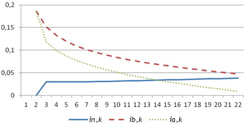
Finally, Table 7 shows the values of the different rates corresponding to the former example. Observe that the rate due to randomness decreases with the number of deposits, 1.6237163% being its average value. The graphic representation of the evolution of the real gross and net average rates, and the average rate due to randomness, can be seen in Figure 3.

Table 7. Average rate due to randomness when the withdrawal of the saved amount is at an agreed date

Age	Year	$i_{b,k}$	$i_{n,k}$	$i_{a,k}$	${ }_1{f}_{k-1}$	$i_{a,k}{\cdot }_1{f}_{k-1}$
50	1	0.18645927	0.00000000	0.18645927	0.02699721	0.005033879
51	2	0.15166648	0.029990308	0.11813332	0.00277555	0.000327885
52	3	0.13239426	0.03000400	0.09940763	0.00217587	0.000216299
53	4	0.11921485	0.029996719	0.08661982	0.00559711	0.000484821
54	5	0.10926625	0.030001682	0.07695576	0.00167278	0.000128730
55	6	0.10130323	0.03000120	0.06922519	0.00234749	0.000162505
56	7	0.09467426	0.03044931	0.06232714	0.00214105	0.000133446
57	8	0.08899677	0.03100857	0.05624415	0.00306079	0.000172151
58	9	0.08402744	0.03156631	0.0508558	0.00336134	0.000170944
59	10	0.07960211	0.03208634	0.04603856	0.00233786	0.000107632
60	11	0.0756048	0.03255879	0.04168868	0.00574866	0.000239654
61	12	0.07195052	0.03311278	0.03759293	0.00467283	0.000175665
62	13	0.06857496	0.03369059	0.03374739	0.00401907	0.000135633
63	14	0.06542817	0.03426394	0.0301318	0.00429169	0.000129316
64	15	0.06247041	0.03481650	0.02672349	0.00667691	0.000178430
65	16	0.05966931	0.03534126	0.02349761	0.00773699	0.000181801
66	17	0.05699795	0.03589115	0.0203755	0.00543752	0.000110792
67	18	0.05443344	0.03644572	0.0173552	0.00739907	0.000128412
68	19	0.05195589	0.03699277	0.01442933	0.00836459	0.000120695
69	20	0.04954756	0.03752506	0.01158767	0.00771624	0.000089413
70	21*	0.04719224	0.03803767	0.00881912	0.88546938	0.007809059
Average						0.016237163

^*For $k=21$, the value of the column ${\hspace{0.17em}}_1^{\hspace{0.17em}}{f}_{k-1}$ corresponds to $p=20$.

Figure 3. Real net average rate, real gross average rate and average rate due to randomness

The expected final deposit, denoted by $\bar{k}$, coincides with the expected termination of the operation analysed in Section 3 since, in this case, the operation finishes with the final deposit. But, in this section, the operation will finish at the date agreed for the withdrawal of the total amount, but the deposits can finish at any time. Thus,

(46) $\bar{k}=E\left[k\right]=\sum _{k=1}^{n-1}k\cdot {\hspace{0.17em}}_1^{\hspace{0.17em}}{f}_{k-1}+n\cdot p_{n-1}$(46)

Analogously, the random date of the final deposit, denoted by $\tilde{k}$, coincides with the financial end of the random operation described in Section 3:

(47) $C_n\cdot p_n\cdot \prod _{h=1}^n{(1+i_h)}^{-1}=\sum _{s=1}^n{a^{\prime }}_s\cdot p_{s-1}\cdot \prod _{h=1}^{s-1}{(1+i_h)}^{-1}=\sum _{s=1}^{\tilde{k}}{a^{\prime }}_s\cdot \prod _{h=1}^{s-1}{(1+i_h)}^{-1}$(47)

5. Conclusion

An important number of developed countries are showing serious maintenance problems of their public pension plans. This leads economic analysts, and even some political leaders, to recommend the population to contract private pension plans which complement the payments received from the public system when they retire. On the other hand, the current financial situation with very low (even negative) rates of interest has forced banks to offer some hybrid products which combine a pure savings operation and an insurance product, usually related with the life of the saver. Therefore, innovation in private savings products is not only convenient but also necessary, to encourage their trading.

In this way, this manuscript proposes two alternatives to traditional savings, based on the probability of survival/death of the saver. In the first one, if the saver dies before the expected end of the operation, the financial institution would benefit from the capital delivered up to that moment and the operation would terminate. Thus, in order to compensate the saver for the assumed risk of loss, the financial institution should make some contributions to the final amount so that, if the saver survived until the agreed end of the operation, he/she would receive an amount greater than the corresponding to a traditional savings operation. Consequently, this operation is attractive for those savers who have no immediate family, since their obtained profitability, in case of survival, is greater whilst the loss, in case of death, is indifferent for him/her.

In the second proposed alternative, the final amount is previously agreed and delivered by the financial institution either to the saver (in case of survival) or to their heirs (in case of saver’s death). However, if the saver dies, the payments to save the final amount would cease. Thus, in this case, the risk is assumed by the financial institution and so the saver would have to pay period amounts greater than the corresponding to traditional savings operations. Therefore, this type of operations is attractive for the saver who has an immediate family to protect economically since his family would receive the same final amount as if he/she does not die without continuing the rest of payments.

The question is whether financial institutions would be interested in offering these operations linked to the investor’s survival. In our opinion, the underlying risk is the same as insurance operations. So, the losses incurred by some operations could be compensated by the benefits generated by others. The question is to estimate the number of operations that the financial institutions should contract so that this loss–profit compensation is effective. It would be necessary to promote an individualized study inside each financial institution, considering the specific risk profile of its clients. To do this, a statistical simulation, based on data about clients and tables of mortality, could be useful to estimate the aggregate profit for banks by considering the two hybrid products presented in this paper. Take into account that the information contained in examples 1 and 3 refers to the payments corresponding to each individual savings product. Moreover, a challenge for banking institution is the bank marketing which is necessary to make attractive these products for consumers. So, banking policy must be oriented to implement the necessary strategies to introduce this novel offer among consumers. Indeed, this would be a future research line.

Summarizing, we believe that a greater offer of savings products would undoubtedly incentivize private savings. Therefore, developing such products is interesting for the future welfare and well-being of the elderly population.

Acknowledgements

We are very grateful for the valuable comments and suggestions offered by an anonymous referee and the journal editor.

Additional information

Funding

This paper has been partially financed by the Project: “La sostenibilidad del sistema nacional de salud: reformas, estrategias y propuestas” [DER2016-76053-R], Programa Estatal de I+D+I Orientada a los Retos de la Sociedad. Ministerio de Economía y Competitividad (Spain).

Notes on contributors

María del Carmen Valls Martínez

María del Carmen Valls Martínez, PhD in Economics and Business, is an associated professor at the University of Almería, Spain. Her research focuses on ethical banking, genre studies, health economics, mathematical analysis of financial operations and anomalies in intertemporal choice. She has published numerous articles in reputable international journals, especially about financial mathematics.

Salvador Cruz Rambaud

Salvador Cruz Rambaud, PhD in Economics and Business, is full professor at the University of Almería, Spain. His current research interests include anomalies in intertemporal choice, mathematical analysis of financial operations and elicitation of new statistical distributions in Finance. He has acted as reviewer of many important journals: International Journal of Uncertainty and Knowledge-Based Systems, Physica A, European Journal of Operational Research, among others.

Emilio Abad Segura

Emilio Abad Segura received his PhD degree from the University of Almería, where currently he is a lecturer.

References

- Balsameda, M., Melguizo, A., & Taguas, D. (2006). Las reformas necesarias en el sistema de pensiones contributivas en España. Moneda y Crédito, 222, 313–340.
- Boldrin, M., Dolado, J. J., Jimeno, J. F., & Peracchi, F. (1999). The future of pension systems in Europe. Economic Policy, 29, 286–323.
- Cesaratto, S. (2002). The economics of pensions: A non-conventional approach. Review of Political Economy, 14(2), 149–177. doi:10.1080/09538250220126492
- Cesaratto, S. (2006). Transition to fully funded pension schemes: A nonorthodox criticism. Cambridge Journal of Economics, 30(1), 33–48. doi:10.1093/cje/bei046
- Clark, R. L., Hanson, E., & Mitchell, O. S. (2016). Lessons for public pensions from Utah’s move to pension choice. Journal of Pension Economics & Finance, 15(3), 285–310. doi:10.1017/S1474747215000426
- Cruz Rambaud, S., & Valls Martínez, M. C. (2014). Introducción a las Matemáticas Financieras. Madrid: Pirámide.
- Danzer, A. M., Dolton, P., & Bondibene, C. R. (2016). Who wins? Evaluating the impact of UK Public sector pension scheme reforms. National Institute Economic Review, 237(1), R38–R46. doi:10.1177/002795011623700115
- Disney, R. (2016). Pension reform in the United Kingdom: An economic perspective. National Institute Economic Review, 237(1), R6–R12. doi:10.1177/002795011623700111
- EU-COMMISSION. (2012). The 2012 Ageing Report-Economic and Budgetary Projections for the 27 EU Member States (2010-2060), 8(1), 73–94.
- Farrell, J., & Shoag, D. (2016). Asset management in public DB and non-DB Pension Plans. Journal of Pension Economics & Finance, 15(4), 379–406. doi:10.1017/S1474747214000407
- Febrero, E., & Cadarso, M. A. (2006). Pay-As-You-Go versus funded systems. Some critical considerations. Review of Political Economy, 18(3), 335–357. doi:10.1080/09538250600797792
- Fernández, S., Vivel, M., Motero, L., & Rodeiro, D. (2012). El ahorro para la jubilación en la UE: Un análisis de sus determinantes. Revista de Economía Mundial, 31, 111–135.
- Fong, J. H., Piggott, J., & Sherris, M. (2015). Longevity selection and liabilities in public sector pension funds. Journal of Risk and Insurance, 82(1), 33–64. doi:10.1111/j.1539-6975.2013.12005.x
- Fontes, A. (2011). Differences in the likelihood of ownership of retirement saving assets by the foreign and native-born. Journal of Family and Economic Issues, 32, 612–624. doi:10.1007/s10834-011-9262-3
- Forman, J. B. (2016). Removing the legal impediments to offering lifetime annuities in pension plans. Connecticut Insurance Law Journal, 23(1), 31–141.
- Hammond, R., et al. (2016). Considerations on state pension age in the United Kingdom. British Actuarial Journal, 21(1), 165–203. doi:10.1017/S1357321715000069
- Harris, M. N., Loundes, J., & Webster, E. (2002). Determinants of household saving in Australia. Economic Record, 78, 207–233. doi:10.1111/1475-4932.00024
- Harrysson, L., Montesino, N., & Werner, E. (2016). Preparations for retirement in Sweden: Migrant perspectives. Critical Social Policy, 4(36), 531–550. doi:10.1177/0261018316638081
- Hira, T. K., Rock, W. L., & Loibl, C. (2009). Determinants of retirement planning behavior and differences by age. International Journal of Consumer Studies, 33, 293–301. doi:10.1111/j.1470-6431.2009.00742.x
- Huberman, G., Iyengar, S., & Jiang, W. (2007). Defined contribution pension plans: Determinants of participation and contribution rates. Journal of Financial Services Research, 31, 1–32. doi:10.1007/s10693-007-0003-6
- Komp, K., & Johansson, S. (2016). Population ageing in a lifecourse perspective: Developing a conceptual framework. Ageing & Society, 36(9), 1937–1960. doi:10.1017/S0144686X15000756
- Lewis, G. B., & Stoycheva, R. L. (2016). Does pension plan structure affect turnover patterns? Journal of Public Administration Research and Theory, 26(4), 787–799. doi:10.1093/jopart/muw035
- Martin, L. G. (2011). Demography and aging (7th ed., pp. 33–45). Handbook of Aging and Social Sciences. London: Academic Press.
- Ni, S., & Podqursky, M. (2016). How teachers respond to pension system incentives: New estimates and policy applications. Journal of Labor Economics, 34(4), 1075–1104. doi:10.1086/686263
- Platanakis, E., & Sutcliffe, C. (2016). Pension scheme redesign a nd wealth redistribution between the members and sponsor: The USS rule change in October 2011. Insurance: Mathematics & Economics, 69, 14–28.
- Seong-Lim, L., Myung-Hee, P., & Montalto, P. (2000). The effect of family life cycle and financial management practices on household saving patterns. International Journal of Human Ecology, 1, 79–93.
- Valls Martínez, M. C., & Cruz Rambaud, S. (2013). Operaciones Financieras Avanzadas. Madrid: Pirámide.
- Valls Martínez, M. C., & Cruz Rambaud, S. (2014). Operaciones realizadas con dos leyes financieras de valoración (pp. 1353–1370). Málaga: XXVIII Congreso Internacional de Economía Aplicada ASEPELT 2014.
- Valls Martínez, M. C., & Cruz Rambaud, S. (2016). Use of two valuation functions in financial and actuarial transactions. Control & Cybernetics, 45(1), 1–14.
- Wang, X. M., Williamson, J. B., & Cansoy, A. (2016). Developing countries and systemic pension reforms: Reflections on some emerging problems. International Social Security Review, 69(2), 85–106. doi:10.1111/issr.12102
- Yang, Z. G. (2016). Population aging and public pension: The case of Beijing analyzed by an OLG model. Singapore Economic Review, 61(4), 1–14. doi:10.1142/S0217590815500459