Metaheuristic algorithm for ship routing and scheduling problems with time window

Abstract

This paper describes a Tabu Search (TS) heuristic for a Ship Routing and Scheduling Problem (SRSP). The method was developed to address the problem of loading cargos for many customers using heterogeneous ships. Constraints include delivery time windows imposed by customers, the time horizon by which all deliveries must be made, and ship capacities. The proposed algorithm aims to minimize the overall cost of shipping operation without any violations. The TS algorithm is compared with a similar method that uses the Set Partitioning Problem (SPP) in terms of solution quality and computational time. The results of a computational investigation are presented. Solution quality and execution time are explored with respect to problem size and parameters controlling the TS such neighborhood size. It is found that while the SPP method solves small-scale problems efficiently, treating large-scale problems with this method becomes complicated due to computational problems; however, the TS method can overcome this challenge. Furthermore, TS consistently returns near-optimal solution within a reasonable time.

Keywords:

• Maritime transportation
• scheduling
• routing
• tabu search
• integer programming

PUBLIC INTEREST STATEMENT

This paper talks about the problem of scheduling the movement of vessels overseas to deliver goods of specific types (such as crude oil or coal) to customers, in the time required by the customer. On the other hand, to reduce the expenses of the movement of the fleet to the lowest possible. These expenses include fuel costs (bunker consumption), operation costs, and port dues. A mathematical algorithm tool called Tabu Search (TS) was presented to create a schedule for a fleet of vessels that could deliver goods to customers in a timely and cost-effective manner.

1. Introduction

The steady growth in international trade over many years has resulted in an increased need for freight transportation. Maritime transportation is the major conduit of international trade, where it plays a key role in international trade as it represents low-cost transportation for high volume and long-distance shipments. The statistics provided by the United Nations Conference on Trade and Development UNCTAD (U. Nation, 2016) show that the world economy heavily depends on seaborne trade. Seaborne trade supports production, trade, and consumption activities by guaranteeing the efficient movement and timely availability of raw materials and finished goods. According to the statistics provided in (U. Nation, 2016) (see Table 1), the total international maritime transportation has increased greatly in terms of weight since 1970. This increase in maritime trade has resulted in parallel growth in the world maritime fleet.

Table 1. World seaborne trade

Year	Total (all shipments)
	Millions of tons loaded
1970	2566
1980	3704
1990	4008
2000	5984
2006	7700
2007	8034
2008	8229
2009	7858
2010	8408
2011	8784
2012	9197
2013	9548
2014	9843
2015	10 047

Ships operate under different conditions than other transportation modes. Christiansen et al. (Christiansen, Fagerholt, & Ronen, 2004) presented these differences: (1) ships pay port dues, (2) ships can be diverted at sea, and (3) a ship’s journey takes days or weeks. Conversely, ships and aircraft share a higher uncertainty in their operations because of their dependence on weather conditions and technology. Therefore, the operational environment of ships differs from the other transportation modes, and ships have different routing and scheduling problems. Christiansen et al. (Christiansen et al., 2004) presented a summary of these differences among other freight shipping modes. Christiansen et al. (Christiansen, Fagerholt, Nygreen, & Ronen, 2013) also presented the most recent review of ship routing and scheduling, where research on ship routing and scheduling problems during the new millennium is reviewed. Certain highlights are that the number of papers doubles every decade, and research on marine inventory routing, liner shipping, and optimal speed is leading the research efforts.

The Ship Routing and Scheduling Problem (SRSP) addressed in this paper involves routing a fleet of controlled and chartered ships, with limited heterogeneous capacities, from an origin to various port customers around the world with known demands and predefined time window constraints. The types of ship investigated in this research are bulk ships which transport raw materials such as iron ore and coal, or tanker ships which transport crude oil, chemicals, and petroleum products. The route cost of a ship consists of fuel costs (bunker consumption), operation costs, and port dues. The objective is to minimize the total cost of serving all cargos while violating no constraint. Routing and scheduling of ships requires a significant level of fleet management planning. Any significant improvement of routing and scheduling will result in substantial cost savings. Cho and Perakis (Cho & Perakis, 2001) presented a mixed integer programming model for the ship scheduling problem with a single loading port. Si-Hwa Kim and Kyung-keun Lee (Kim & Lee, 1997) considered the ship owner’s scheduling problem in bulk trade and solved it using a set-packing model. The model sought to maximize the net profit. Gatica and Miranda (Gatica & Miranda, 2011) developed a network-based model for the routing and scheduling of a heterogeneous fleet. The objective is to minimize the total operating cost of serving a set of trip cargo contracts considering time window constraints at both the origin and destination of cargos. Brønmo et al. (Brønmo, Christiansen, & Nygreen, 2007b) used integer programming to solve the problem. All feasible routes are generated priori, where the optimal cargo quantities are found by solving a linear programming problem. The solution for the SRSP is solved using a SPP. Brønmo et al. (Brønmo, Nygreen, & Lysgaard, 2010) used branch-and-price to generate columns during the solution process. Andersson et al. (Andersson, Duesund, & Aderholt, 2011) present a mathematical formulation for a tramp ship routing problem. The researchers proposed three alternative solution methods based on path flow formulations and a priori column generation, where the objective is to maximize the profit.

All the above approaches are capable of producing feasible solutions for SRSP. However, the simplest problem in routing and scheduling has high computational complexity, as evidenced by solution times of exact algorithms. Therefore, due to the exponential size of the solution space, it is unlikely that these optimization procedures can be used for large-scale problems. Heuristic methods, such as Simulated Annealing (SA) (Kirkpatrick, Gelatt, & Vecchi, 1983), Genetic Algorithm (GA) (Holland, 1975), or Tabu Search (TS) (Glover, 1986), which produce optimal or near-optimal solutions with acceptable computational time, are attractive alternatives. To our knowledge, there is minimal research work on SRSP using heuristic methods; most published works focus on Vehicle Routing and Scheduling (VRS). Moon et al. (MoonCorrespondence, Qiu, & Wang, 2014) used the GA to address a tramp ship routing model of fleet deployment in a hub-and-spoke network. Many random generated problem instances were solved using a mathematical programme and the GA with local search. A comparison of the results showed the efficiency of the GA with local search. Alhamad et al. (Al-Hamad, Al-Ibrahim, & Al-Enezy, 2012) also addressed SRSP using GA. The representation of each chromosome is an integer string of the number of shipments in the problem, while each gene is the integer number of a specific ship assigned to that original shipment. The objective is to minimize the overall operation cost. Sherali et al. (Sherali, Al-Yakoop, & Hassan, 1999) presented an industrial SRSP, where the cargo owner controls the fleet of ships and no optional spot cargos, which makes it different from the paper presented here. The objective is to minimize the overall cost.

Korsvik and Fagerholt (Korsvik & Fagerholt, 2010) used TS to solve ship the routing and scheduling encountered by many tramp shipping companies transporting bulk products, where the objective is to maximize the profit instead of minimizing the overall costs as in this paper. The researchers used TS to help the planner to determine the optimal cargo quantities in each route. The computational results showed that optimal or near-optimal solutions for real-life cases were produced within a reasonable time.

The shipping operations planner needs to frequently reschedule within a very short time frame, since ocean shipping is a very dynamic business. The main contribution of this research is to develop an efficient TS algorithm for the SRSP with flexible cargo quantities and to serve all customers with no violation of the constraint and with minimum overall cost.

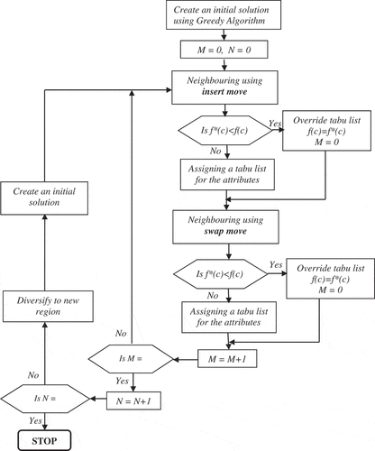
Tabu search (TS), proposed and developed by Glover (Glover, 1986), is a memory-based search strategy that guides the local search to continue its search beyond the optimum local solution. This procedure occurs by storing the most recently visited solutions in a tabu list (forbidden list) for a number of iterations to prevent any repletion or cycling. The lifetime moves that remain in the tabu list is called tabu tenure, and it could be a variable or fixed size. The control rule to refresh the tabu list is first-in first-out for the moves that are entered into the tabu list. However, a specific move or solution can be overridden in the tabu list when the move leads to a solution better than any currently available solutions. This condition is called aspiration criteria. TS begins by generating an initial solution, and the investigation uses an insert and swap move to search an optimal or near optimal solution. Moreover, to improve the solution, intensification and diversification mechanisms are used. Intensification more carefully explores the region that has previously been visited, while diversification forces the steering search to unexplored areas of the search space. To measure the quality of this TS heuristic method, an exact method is used by adapting the Set Partitioning Problem (SPP) for small-scale problems.

This paper is arranged as follows: section 2 presents a mathematical formulation of SRSP. Section 3 provides information regarding using TS with insert and swap moves where intensification and diversification techniques are used. Section 4 provides the methodology of the exact approach SPP. Overall computational results and analysis are presented and described in section 5. Finally, conclusions are provided in section 6.

2. Mathematical formulation

The SRSP addressed here is defined as each of a given number of ships with different capacities that will serve one or more cargos on each trip, where each ship can make more than one trip within the time horizon, and where the route for a specific ship is the total of all trips the ship has made. The requirements of all cargos must be satisfied. Each cargo has an imposed delivery time window according to the agreed contract with the company. Unloading must occur within the delivery time window. If the ship arrives before the time window, it must wait until the start of the delivery time window before unloading. The objective function, which seeks to minimize the overall cost, considers all the transportation expenses, fuel consumption, crew wages, maintenance, fixed cost of chartered ship, and other expenses.

This problem is defined formally as follows: NC is a set of vertices (cargos), $i=\left\{0,1,...,NC\right\}$, where 0 is the origin, and NC is the total number of cargos to be served. There is a set of ships, NS, where $N{S}_{v1}$ is the total number of controlled ships belonging to the company with different capacities and the same speed. $N{S}_{v2}$is a fleet of chartered ships, where the company can resort to the market to charter if there are insufficient ships to deliver all cargos. It is assumed that all chartered ships will be available at the beginning of the schedule. The total number of all ships used is $NS=N{S}_{v1}+N{S}_{v2}$.

Let schedule $S=\left\{(i,k):i\in NC,k\in NS\right\}$, which means that cargo i is served by ship k, where all constraints are satisfied. Consider, for example, 5 cargos are served using 2 ships, A and B, as shown in Figure 1.

Figure 1. Example of schedule of 2 ships serving 5 cargos.

The route of ship A states that the ship loaded from the origin (zero) to serve cargo 3 then returns to the origin to load cargo 4 then returns to the origin. The route of ship B proceeds in the same manner as the route of ship A to serve cargos 1, 2, and 5.

Cargo i can be served only once by ship k from either controlled or chartered ships. Ship capacities are different, and cargo i has demand. This statement assumes that there is sufficient capacity available to satisfy all cargo demands. Each cargo has predefined time window. Time window constraints are presented by an earliest arrival time and a latest arrival time.

3. Tabu search

The SRSP is solved using the TS method, proposed and developed by Glover (Sherali et al., 1999). The most important characteristic of TS is the use of memory for the solution to solve difficult problems. There are many techniques used in TS such as attributes, tabu list, tabu list size (tenure), intensification, diversification, neighborhood, and neighborhood size, move and evaluation of the move, all which are adapted in our approach. Parameters defining the neighborhood size N.size and the tabu list size are considered critical in terms of solution quality and computation time. The most important point in a TS is the need for experimentation to choose the best parameters and their values for each specific type of problem.

The methodology of solving this problem begins by arranging all cargos in sequence according to their departure time from the origin to serve them. Therefore, the cargo with the earliest departure time will be considered cargo number one and so on for other cargos. Thereafter, an initial solution will be generated to begin seeking the solution.

3.1. Initial solution

The initial solution $s_o$is constructed using a greedy algorithm, which is a practical and straightforward algorithm. A greedy algorithm is implemented by first selecting the lowest overall cost ship among all fleets of ships according to the operation cost. Second, a route is created for this ship starting from cargo number one. At the same time, all constraints are satisfied, such as capacity and delivery time window. Once the first selected ship has finished, the same procedure for the second cheapest cost overall ship will be implemented, until no cargo remains. Any remaining cargo will be assigned to spot the ship, which is costly.

Greedy Algorithm.

1. Until number of $n_c$= 0

2. set $n_c$= $NC$

3. set count = 0

4. choose k, where $k\in NS$, $k$ is the cheapest and $k\notin$hold

5. Select cargo $i$, where $i\notin served$,

6. If $k$ satisfies all constraints, then

cargo $i$ served by ship $k$, $i\in served$

count = count + 1

$n_c$= $n_c$– 1

If count $\le n_c$, then

go to (5)

Else, $k\in$hold

go to (3)

(7) End Until

The result is illustrated in Table 2:

Table 2. Schedule for all cargos with their ships

cargo	1	2	…………..	n
Ship	D	A	…………	k

where cargo 1 is served by ship D; cargo 2 is served by ship A, and so on, until the last cargo n is served by ship k.

The following section explains the methodologies of solving this type of problem using the TS method and separately describes the characteristic of each component of the method.

3.2. The neighbourhood structures

The idea behind generating neighboring solutions is to improve the initial solution to the optimal or near optimal solution, where an initial solution $s_o$is constructed using a greedy algorithm. Then, each solution $s_o\in S$ is associated with an attribute set $A(s)=\left\{(i,k):i=1,...,NS;\right.$ $\left.k=1,...,NC\right\}$, where (i,k) means that cargo i is served using ship k. The construction of the neighborhood for initial solution $s_o$ is implemented using two operator moves, insert and swap moves. The methodology of insert move operates by deleting attribute (i,k) from set A(s) and attempts to replace it with another attribute (i,k’). This methodology means that cargo i is removed from ship k and assigned to another ship k’ where $k\ne k^{\prime }$. Inserting cargo i in the route of ship k’ is executed to minimize the overall cost f(c). There are several approaches for insert move, where the process can delete one, two, or three cargos from the ship’s route and attempt to insert them into another ship’s routes, which, in this paper, are named 1-insert, 2-insert, and 3-insert move mechanisms.

The insert process begins from the first cargo in ship k’ route, where the insert trail assigns cargo i into position $i{\prime }^{-}$. If constraints are not satisfied, the insert trail will carry on to position $i{\prime }^{+}$(minus and plus signs are the position order before or after cargo $i^{\prime }$). If the attempt fails, the process continues to the second cargo $i^{\prime \prime }$using the same procedure, and so on, until the last cargo in the route. If ship k’ cannot hold cargo i, the insert trail will transfer to ship k’’ until the last ship; otherwise, cargo i will be assigned to spot ship. The 1-insert, 2-insert, and 3-insert move mechanisms adopted in this paper produce a suitable solution, while they take more computational time in the delete-insert procedure. Figure 2 illustrates several types of insert moves.

Figure 2. The insert move procedure with three types of move mechanisms: 1-insert, 2-insert, and 3-insert.

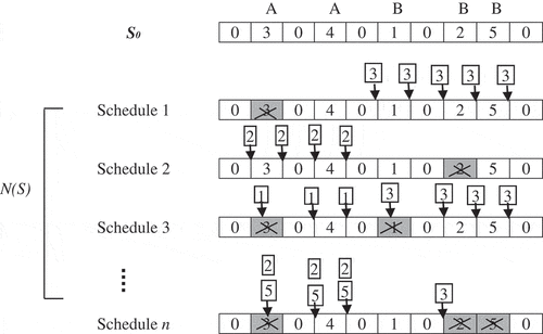
Comment: If two or more cargos are deleted from the route of ship k (as Schedule n, where cargos 2 and 5 are deleted), the first cargo will be selected randomly, and the next will be inserted into the route of ship k’. The same procedure applies for the second cargo and so on. For example, in Figure 2, the first cargo selected to be inserted into ship route A is 5; the next is cargo 2.

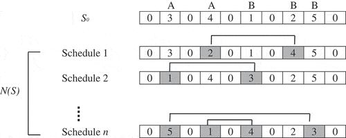
The swap operator exchanges the position of two or more cargos. This swap removes two attributes (i,k) and (j,k’), where $i\ne j$ and $k\ne k^{\prime }$, from A(s) and interchanges them with two new attributes, (i,k’) and (j,k).

If three cargos are selected, (i,k), (i’,k’), and (i’’,k’’), where$i\ne i^{\prime }\ne i^{\prime \prime }$, and $k\ne k^{\prime }\ne k^{\prime \prime }$, the swap operation will be operated as (i’’,k), (i,k’), and (i’,k’’). All constraints must be satisfied, such as loading and unloading time windows or the capacity of the ship. Any infeasible schedule will be rejected. Furthermore, the schedule with the lowest overall cost f(c) will be chosen. Figure 3 illustrates the swap operator procedure.

Figure 3. The swap move procedure.

When the insert operation is completed in that ship route, the attribute (i,k) will be forbidden for a number of iterations (or (i,k) and (j,k’) for the swap operator). That statement means that attribute (i,k) will be assigned as a tabu status (tabu list). A tabu list usually consists of a list of moves the search has recently encountered. The moves on the tabu list cannot be revisited for a particular number of iterations called tabu tenure (tn of iterations). The tabu list helps the search to move from a previously visited section of the search space and to execute more extensive exploration. In this model, there are two tabu lists, one for the insert move and the other for the swap move. Moreover, the value of tabu tenure could be fixed or set as a variable, in this paper, the tabu tenure was set as a variable. However, move that remain in the tabu list for long periods of time may restrict the search process from proceeding and may cause to end sooner. Therefore, tabu tenure tn is fixed at 7–11 iterations. Conversely, this restriction can be revoked (canceled) by an aspiration criterion, for either insert or swap, if that move allowed the search to reach a solution with an overall cost f*(c) smaller than the best solution ever obtained.

Number of neighborhood is considered a critical point in the moves operation. If the number of neighborhood is excessively small, it will restrict the search; a suitable solution is less likely to be found. Conversely, if the number of neighborhood is excessively large, it loses its purpose of diminishing the neighborhood size. A suitable trade-off can be obtained by experimentation.

To use the TS heuristic method, there are three types of decision variables to solve SRSP (Figure 4). The first decision variable is$r_{ik}$, where $i\in NS$ and $k\in NC$, is 1 if cargo i is served by ship k, and 0 otherwise. $w_{ik}$, the second decision variable, denotes the actual arrival time for ship k serving cargo i. The last decision variable is $f(c)$, which denotes the overall cost serving all cargos.

Figure 4. Flowchart of the TS process.

Decision variables:

$r_{ik}\in 1,0$	=	1 if cargo i is on the route of ship k, and 0 otherwise.
$w_{ik}$	=	actual arrival time for ship k serving cargo i.
$f(c)$	=	total cost serving all cargos.

Parameters:

$NS$	=	total number of ships, where ship $k\in \left\{1,2,...,NS\right\}$,
$NC$	=	total number of cargos, where cargo $i\in \left\{1,2,...,NC\right\}$,
$T_i$	=	travel time (days) from origin to cargo i,
$T_{ij}$	=	travel time (days) from port of cargo i to port of cargo j,
$e_i$	=	earliest start time of the delivery of the cargo i,
$l_i$	=	latest finish time of the delivery of the cargo i,
$l{d}_i$	=	time (days) to load cargo i,
$u{d}_i$	=	time (days) to unload cargo i,
$q_k$	=	capacity of ship k,
$A{v}_k$	=	availability of ship k at origin,
$d_i$	=	quantity of cargo i,
$p{d}_i$	=	port due at customer of cargo i,
$c{v}_k$	=	operating cost per day for ship k in journey,
$a{v}_k$	=	available time for ship k at origin,
$C_{ik}$	=	the cost of serving cargo i using ship k,
$InTer$	=	denotes the number of iterations needed to search in the current region, where $\theta \in InTer$
$DivIter$	=	denotes the number of times the search diversifies into a new region,

The variable of actual arriving time $w_{ik}$ to deliver cargo i using ship k can be computed using one of the following two equations:

(1) $w_{ik}=a{v}_k+l{d}_i+T_i$(1)

(2) $w_{ik}=e_i,\mathrm{I}\mathrm{f}a{v}_k+l{d}_i+T_i<e_i$(2)

Equation (1)(1) $w_{ik}=a{v}_k+l{d}_i+T_i$(1) means that ship k arrived within the delivery time window of port i, $w_{ik}\in [e_i,l_i]$. Conversely, equation (2)(2) $w_{ik}=e_i,\mathrm{I}\mathrm{f}a{v}_k+l{d}_i+T_i<e_i$(2) means that ship k arrived at port i before the earliest start time; then ship k can be delayed and yet comply with the delivery time window at port i.

The cost $C_{ik}$ for cargo i using ship k can be computed by:

$C_{ik}=p{d}_i+c{v}_k{T}_i$

This equation includes the port due of cargo i plus the overall cost for the number of days ship k has consumed to deliver cargo i.

Finally, the total cost $f(c)$ for this problem can be counted by:

$f(c)=\sum _k^{NS}\sum _i^{NC}{C}_{ik}{r}_{ik}$

This equation computes the overall operation cost to deliver all cargos using a number of ships.

3.3. The candidate list of elite solutions

During the process, the long-term memory of TS stores elite solutions the system has determined, where these solutions are stored in Candidate list. Storing this solution is according to the best value of the overall cost $f(c)$, where the best one will be in the front of the configuration of the candidate list. Since the size of the candidate list is a variable, certain solutions leave candidate list once better solutions enter the list. The purpose of storing elite solutions in the candidate list is to use them in the diversification phase.

3.4. The intensification and diversification

In designing a meta-heuristic, two criteria need to be considered: intensification and diversification. In intensification, the promising regions are explored more thoroughly, hopefully to find better solutions. Conversely, in diversification, non-explored regions must be visited to be certain that all regions of the search space are consistently explored and that the search is not restricted to only a reduced number of regions. The insert and swap moves’ operation generates many solutions by searching the current region, to explore more in the current region. The intensification technique is applied as follows; if the search yields the best solution thus far, the search in this region will start over, where the current iteration $\theta =0$, and the search proceeds to search more thoroughly. This statement means that this area appears to be attractive. Once this region has been searched for a number of iterations equal to $InTer$with no improvement of the solution quality, it is time to diversify the search to discover other regions. This diversification provides the opportunity to investigate another region and to avoid trapping the search in a small space. This mechanism drives the search process towards less explored regions of the solution space whenever a local optimum is attained.

TS in this paper begins with an initial solution obtained from the Greedy algorithm, as noted previously. Once this region has attained the optimum of its neighborhood, then it is time to search in another region. To encourage this method to explore previously unvisited regions of the search space and minimize the risk of surrounding in local optima, a diversification technique is adopted.

This technique used in this algorithm is a transition-based long-term memory that is utilized to store the frequency of movements after each move: insert or swap. To divert the search to an unexplored region, any attribute (i,k) is frequently entered into the tabu list during the search; this will be penalized by the following function:

$P_{ik}=\gamma .n{t}_{ik}/\eta$

where $n{t}_{ik}$indicates the number of times attribute (i,k) is entered into the tabu list during the search process, and $\eta$ represents the current diversification number. The parameter $\gamma$ is used to manage the intensity of the diversification. These penalties will control the diversification of the search process towards less explored regions of the solution space. The procedure is conducted by displaying all or a subset of the elite solutions stored in the candidate list. The swap move will be applied between each of the two strings of elite solutions randomly. Any attribute (i,k) with $P_{ik}\ge over$will be forbidden from entry into the configuration of the new solution. Once the new solution $s$is constructed, then the neighborhood N(s) of the new solution $s$will be constructed using the same two neighborhood operators: insert and swap. The searching process in this region will be conducted using the same procedure as the previous region for a number of iterations $InTer$. The diversifying will continue to other unexplored regions for a number of times equal to $DivIter$. This periodic diversification has proven to be very effective for this type of problem, which is tightly constrained. Furthermore, if the number of $DivIter$is large, a suitable solution could be obtained, while the computation time is increased tremendously. The best trade-off for the number of $DivIter$ according to experiments is equal to 200; the best solutions rarely occur beyond this number. The algorithm terminates once the diversification has attained the number of $DivIter$with no improvement in the solution quality.

4. Exact approach

To solve this type of problem by using an exact algorithm, the first step is to generate all feasible schedules for each ship, where all constraints are satisfied. Then, we apply the (SPP) optimization method. To demonstrate the method of generating all the proposed schedules for each ship, see Table 2.

The schedule consists of a route that consists of a sequence of pickup and delivery nodes. The pickup node refers to the origin, while the delivery node refers to cargo-port. Table 3 illustrates a number of candidate schedules generated for ship k to serve 3 cargos. Each schedule must satisfy a number of conditions to be accepted as a feasible candidate schedule; otherwise, it will be deleted. Therefore, all feasible schedules will be considered a set of feasible schedules $S_k$for ship k. The following conditions must be tested in case there is only one cargo in this schedule:

(3) $d_i\le q_k$(3)

(4) $A{v}_k+l{d}_i+T_i\le l_i$(4)

Table 3. Number of candidate schedules for ship k to serve 3 cargos

s	Route	s	Route	s	Route
1	0–1–0	14	0–2–0	27	0–3–0
2	0–1–2–0	15	0–2–1–0	28	0–3–1–0
3	0–1–0–2–0	16	0–2–0–1–0	29	0–3–0–1–0
4	0–1–3–0	17	0–2–3–0	30	0–3–2–0
5	0–1–0–3–0	18	0–2–0–3–0	31	0–3–0–2–0
6	0–1—2—3–0	19	0–2—1—3—0	32	0–3—1—2–0
7	0–1—2—0–3—0	20	0–2—1–0–3—0	33	0–3—1—0–2—0
8	0–1—0–2—3—0	21	0–2—0–1—3—0	34	0–3—0–1—2—0
9	0–1—0–2—0–3—0	22	0–2—0–1—0–3—0	35	0–3—0–1—0–2—0
10	0–1—3—2—0	23	0–2—3—1—0	36	0–3—2—1—0
11	0–1—3—0–2—0	24	0–2—3—0–1—0	37	0–3—2—0–1—0
12	0–1—0–3—2—0	25	0–2—0–3—1—0	38	0–3—0–2—1—0
13	0–1—0–3—0–2—0	26	0—2—0—3—0—1—0	39	0—3—0—2—0—1—0

where condition (3) assures that the capacity of ship k is more than or equal to the quantity of cargo i. In condition (4), the arrival time at the delivery node of cargo i is not to exceed the latest completion time of delivery. After confirming these two conditions, the cost of this schedule will be calculated as the first schedule of this specific ship.

In case there are 2 cargos to be served, the following conditions must be satisfied:

(5) $d_i+d_j\le q_k$(5)

(6) $A{v}_k+l{d}_i+l{d}_j+T_i\le l_i$(6)

(7) $A{v}_k+l{d}_i+l{d}_j+u{d}_i+T_i+T_{ij}\le l_j$(7)

Condition (5) confirms that ship k can hold cargo i and j simultaneously in the same route for ship k, without violating ship capacity; for an example, see s = 2 in Table 3. This finding means two sequence delivery nodes are generated for ship k. Furthermore, conditions (6) and (7) guarantee the delivery for both cargos will not violate the delivery time window for each cargo.

Conversely, if one of the previous conditions is not satisfied, which means the sequence delivery nodes are not permitted, the following conditions will be tested:

(8) $d_i\le q_k\mathrm{a}\mathrm{n}\mathrm{d}{d}_j\le q_k$(8)

(9) $A{v}_k+l{d}_i+T_i\le l_i$(9)

(10) $A{v}_k+l{d}_i+T_i+u{d}_i+T_i+l{d}_j+T_j\le l_j$(10)

where condition (8) assures that the capacity of ship k is more than or equal to the quantity of cargo i and cargo j individually. This finding means that cargo i will be delivered first, then ship k will return to the origin to load cargo j. Conditions (9) and (10) test the capability of ship k to load and unload cargo i then return to pickup node -origin- to load cargo j, without violating the delivery time window for both cargos.

The same procedure will be conducted for the remaining cargos using the same conditions until no cargo remains. Furthermore, if any schedule does not satisfy one of these conditions, that schedule will be deleted. Also, two or more schedules for a specific ship k have the same cargos in their route but in different configurations; for an example, see s = 11, 25, and 33 in Table 3. If overall cost f(c) is the same, one schedule will be considered, while the remainder will be deleted. Conversely, if the overall costs are not the same, the lowest overall cost f(c) will be considered. This procedure will minimize the number of feasible schedules $S_k$for ship k, which reduce the computation time.

There is one set of decision variables $x_{ks}$ to solve SPSP, where it is 1 if schedule s is selected for ship k, and 0 otherwise. The objective is to minimize the overall cost $c_{ks}$. Furthermore, all cargos are served by using the available fleet of ships where all constraints are satisfied. The following formula will be applied to solve this problem:

(Exact formulation by SPP)

Decision variables:

$x_{ks}\in \left\{1,0\right\}$, 1 if schedule s is selected for ship k, and 0 otherwise.

Parameters:

$NC$	=	total number of cargos, where cargo $i\in \left\{1,2,...,NC\right\}$,
$S_k$	=	set of feasible schedules for ship k,
$a_{ksi}$	=	if cargo i in schedule s is served by ship k, where $s\in S_k$,
$c_{ks}$	=	overall cost for schedule s using ship k, where $s\in S_k$,

Minimize

(11) $\sum _k\sum _{s\in S_k}{c}_{ks}{x}_{ks}$(11)

Subject to

(12) $\sum _{s\in S_k}{x}_{ks}\le 1\mathrm{\forall }k\in NS$(12)

(13) $\sum _k\hspace{0.17em}\sum _{s\in S_k}{a}_{ksi}\ast x_{ks}=1\mathrm{\forall }i\in NC$(13)

$x_{ks}\in 0,1$

Expression (11) is the objective function of the problem minimizing the overall operation cost. Constraint (12) limits each ship to sailing at most one route within the time horizon. Constraint (13) ensures that every cargo will be loaded.

This optimization procedure can be used for two purposes. First, the exact approach will be used as a comparison with the TS heuristic method in terms of the solution quality and the computational time, while the second purpose is use for small-scale problems.

5. Experiments and analysis

The TS heuristic method and the column generation model were coded and implemented using Visual Basic 6, while the exact algorithm SPP is implemented using CPLEX-10. The PC used is Fujitsu LifeBook A557 Core i5-7200U 4GB 500GB 15.6 Inch.

Efforts have been made to obtain information on this subject from Kuwait Oil Tanker Company (KOTC); however, the management apologized for the confidentiality of information. Therefore, ship time availability, ship capacity, cargo duration, cargo quantity, and cargo delivery time window are all generated from a uniform distribution shown in Table 4 for the fleet of ships and Table 5 for cargos.

Table 4. Uniform distribution for a fleet of ships

Controlled Ships		Chartered Ships
Ship capacity (tons)	Time availability (days)	Ship capacity (tons)	Time availability (days)
(100,460)	(1,60)	(100,460)	Exact 1

Comment: Time availability for chartered ships is in the first day, which presumed that the company should be chartered previously before the start constitutes the schedule.

Table 5. Uniform distribution of cargos

Cargo
Duration (days)	Volume (tons)	Earliest arrival time [$e_i$] (days)	Latest arrival time [$l_i$](days)
(4,60)	(100,600)	30 + U[1,T]	$e_i$+ U[3, 20]

Setting the parameters of the TS is essential in achieving a suitable performance. After experimentations, the parameters for the TS are set as follows: the quantity of tenure tn is in the range (Andersson et al., 2011; Brønmo et al., 2007b, 2010; Holland, 1975; Kirkpatrick et al., 1983). The quantity of iterations IterAll is equal to 10,000 iterations, while the best trade-off for the quantity of $DivIter$ according to experiments is equal to 200.

The major parameter for TS that will be analyzed is the neighborhood size, N.size. Then, to measure the quality of the TS solution, a comparison will be implemented using the SPP approach solutions in term of quality of the solution and computation time.

5.1. Neighbourhood size (n.size)

To measure the best Neighbourhood size, N.size, a problem with 100 cargos and 55 ships (42 controlled and 13 chartered) and a time horizon of 150 days was generated randomly. Each problem was examined by three different neighborhood sizes, N.size= 30, 40, 50, with 100 replicates generated for each.

The computational results are summarized in Table 6 for different problem sizes. This table indicates that the best value of N.size is equal to 50, which is clear in Table 6. When N.size = 50, we frequently achieved the best solution 23 times.

Table 6. Neighbourhood size for problem 2

N.Size	12	16	20	24	32	36	40	50	60
Frequency	1	8	9	8	13	12	14	23	12

The main idea behind heuristic methods is to solve large-scale problems, since the exact approach SPP cannot solve them, where SPP used in this paper is capable of solving small size problems. Ten different problem sizes were applied to measure the capability of the TS of solving large problems; 25 replicates were generated for each. The size of N.size, which was proved previously, was adopted. Table 7 presents an indication that, if the size of the problem increases, the time to obtain the solution increases as well. Thus, solving the problems of 300 cargos took an average of 10,316 s (approximately 3 h), which notifies the reader that problems such as 500 cargos may take a long time to be solved. This slow solution issue can be avoided by reducing N.size, with the solution not being as extensive as when using the same values of the TS parameters examined previously.

Table 7. Comparison between number of cargos and time consumption to obtain solution

Number of cargo	50	75	100	125	150	175	200	225	250	300
Mean (time-sec)	18.67	64.67	171.8	386	764.8	1552	2847	3849	5592	10,316
StDev. (time-sec)	1.359	2.38	9.234	12.39	39.98	75.46	180.8	134.6	138.6	518.3

Furthermore, Intensification played a significant rule in this method, where the search was re-started several times in the search neighborhood. This result shows that a lower overall cost than the best solution thus far has been found. Conversely, diversification enhanced the quality of the solution, where halting the mechanism of diversification yields a non-attractive solution. Furthermore, for the diversification mechanism, the best value for the parameter$\gamma$is in the range (Andersson et al., 2011; Brønmo et al., 2007b, 2010; Gatica & Miranda, 2011), which has proven to be very effective for this type of problem.

5.2. Comparison of computational results

In this section, the comparison of the two approaches proposed for solving this problem is presented. Both models, TS and SPP, used the same objective function for comparison. The objective of the experiments is to evaluate the performance of TS in terms of the quality of the solution and the computation time.

Applying five different size problems (20, 24, 28, 32, and 36 cargos), as presented in Table 8, showed that the percentage of the solution quality by using TS and SPP is not that large; however, in a problem with 20 cargos the percentage gap between the objective function of TS and SPP is 2.2%. For the last one, the gap is also not that large, 4.4% for a problem size of 36 cargos. This finding provides an indication that the results are near optimal, and at the same time, the user can resort to the TS model to solve a large problem. Conversely, in Figure 5, the time increased rapidly when using SPP, while the time consumption when using TS is small. At the same time, since the personal computers are constrained by memory space, and the number of variables (candidate schedules) are increasing rapidly (more than 500 thousand variables for a problem with 36 cargos), this currently makes it very difficult to solve this type of problem with this number of variables. This indication provides the user in a shipping company with the flexibility to determine when they can use the exact approach or the heuristic method.

Table 8. Computational results for problem sizes 20–36

Problem size	TS	SPP		Differences
	Average Time for solution (second)	Average No. of Variables	Average Time for solution (second)
20	0.6	9752.9	2.52	2.2%
24	1.28	23,541.4	6.51	3.015%
28	3.1	65,907.7	27.912	3.55%
32	4.4	137,471.3	52.45	3.71%
36	5.2	528,274.8	435.8	4.4%

Figure 5. Computational times between SPP and TS (CPU [s]).

6. Conclusion

In this research, a TS algorithm was presented to address the ship routing and scheduling problem, faced by a fleet of controlled and chartered ships of type bulk or tankers, with limited heterogeneous capacities, from an origin to various port customers around the world with known demands and predefined time window constraints. The route cost of a ship consists of fuel costs (bunker consumption), operation costs, and port dues. The objective is to minimize the total cost of serving all cargos while violating no constraint. TS algorithm is capable of finding a near-optimal solution for SRSP in a very short computing time compared with the exact algorithm SPP (column generation approach); both were presented. The computational study shows that the TS heuristic quantity optimization returns a high-quality solution. The computational time is significantly less for the TS than for the exact algorithm. It was determined that TS N.size plays an important role in this heuristic model. Conversely, this paper presented that a company dealing with less than 36 cargos can use the SPP model to obtain an optimal solution, while for companies with more than 36 cargos, it is recommended that a company use TS, which is very fast and offers a reasonably suitable solution. On the other hand, shipping companies often minimize the overall cost, which in turn maximizes the profit. This technique and not the traditional manner (ad hoc) will achieve this goal in a reasonable time and using a scientific method.

Additional information

Funding

This work was supported by the Khaled Moh Alhamad.

Notes on contributors

Khaled Alhamad

Khaled Alhamad is currently an associate professor, PhD and Head of Laboratory Technology Department, College of Technological Studies, Kuwait. His research interests include optimization, integer programming, heuristic method, scheduling, transportation.

References

- Al-Hamad, K., Al-Ibrahim, M., & Al-Enezy, E. (2012). A genetic algorithm for ship routing and scheduling problem with time window. American Journal of Operations Research, 2(3), 417–16. doi:10.4236/ajor.2012.23050
- Andersson, H., Duesund, J., & Aderholt, K. (2011). Ship routing and scheduling with cargo coupling and synchronization constraints. Computers & Industrial Engineering, 61, 1107–1116. doi:10.1016/j.cie.2011.07.001
- Brønmo, G., Christiansen, M., & Nygreen, B. (2007b). Ship routing and scheduling with flexible cargo size. Operational Research Society, 58(9), 1167–1177. doi:10.1057/palgrave.jors.2602263
- Brønmo, G., Nygreen, B., & Lysgaard, J. (2010). Column generation approaches to ship scheduling with flexible cargo sizes”. European Journal of Operational Research, 200, 139–150. doi:10.1016/j.ejor.2008.12.028
- Cho, S.-C., & Perakis, N. (2001). An improved formulation for bulk cargo ship scheduling with a singlr loading port”. Maritime Policy and Management, 28, 339–345. doi:10.1080/03088830010002755
- Christiansen, M., Fagerholt, K., Nygreen, B., & Ronen, D. (2013). Ship routing and scheduling in the new millennium. European Journal of Operational Research, 228, 467–483. doi:10.1016/j.ejor.2012.12.002
- Christiansen, M., Fagerholt, K., & Ronen, D. (2004). Ship routing and scheduling: Status and perspectives. Transportation Science, 38(1), 1–18. doi:10.1287/trsc.1030.0036
- Gatica, R. A., & Miranda, P. A. (2011). Special issue on Latin-American research: A time based discretization approach for ship routing and scheduling with variable speed. Networks and Spatial Economics, 11(3), 465–485. doi:10.1007/s11067-010-9132-9
- Glover, F. (1986). Future paths for integer programming and links to artificial intelligence. Computers and Operations Research, 13, 533–549. doi:10.1016/0305-0548(86)90048-1
- Holland, J. H. (1975). Adaption in natural and artificial systems. Ann Arbor, MI: University of Michigan Press.
- Kim, S.-H., & Lee, -K.-K. (1997). An optimization-based decision support system for ship scheduling. Computer and Industrial Engineering, 33, 689–692. doi:10.1016/S0360-8352(97)00223-4
- Kirkpatrick, S., Gelatt, J., & Vecchi, M. P. (1983). Optimization by simulated annealing. Science, 220, 671–680. doi:10.1126/science.220.4598.671
- Korsvik, J., & Fagerholt, K. (2010). A tabu search for ship routing and scheduling with flexible cargo quantities. Journal of Heuristics, 16, 117–137. doi:10.1007/s10732-008-9092-0
- MoonCorrespondence, I. K., Qiu, Z. B., & Wang, J. H. (2014). A combined tramp ship routing, fleet deployment, and network design problem. Maritime Policy & Management, 42, 68–91.
- Sherali, H. D., Al-Yakoop, S. M., & Hassan, M. M. (1999). Fleet management models and algorithms for oil-tanker routing and scheduling problem. IIE Transactions, 31, 395–406. doi:10.1080/07408179908969843
- U. Nation. (2016). Review of maritime transportation. United Nations Conference on Trade and Development (UNC-TAD). Retrieved from https://unctad.org/en/PublicationsLibrary/rmt2016_en.pdf