A test of Wagner’s hypothesis for the Ghanaian economy

Abstract

The economy of Ghana profiles a trajectory of increasing government expenditure at the backdrop of an inconsistent growth in real GDP. Thus, this study explores the causal relationship between real economic growth and real government expenditure in Ghana between the period 1960 to 2017. The Johansen (1991, 1995) cointegration method, the Autoregressive Distributed Lag bounds test approach and the Toda-Yamamoto non-Granger causality test are employed in this study. The findings are that the variables are cointegrated, and there is no Granger causality from real economic growth to real government expenditure. In effect, the causality shows that the Wagner’s hypothesis does not hold in the case of the Ghanaian economy and that the Keynesian theoretical standpoint that public expenditure is an exogenous factor is not deflated in this case.

Keywords:

• Wagner’s hypothesis
• economic growth
• cointegration
• Granger causality
• autoregressive distributed lag model
• Ghana

PUBLIC INTEREST STATEMENT

This study explores the causal nexus between real public expenditure and real economic growth. The implication is that the study helps policymakers to ensure government derives value for money spent by directing government expenditures to the most productive sectors of the Ghanaian economy. It is therefore suggested that the government puts measures in place to ensure effective government expenditure governance.

1. Introduction

Since the introduction of Wagner’s law in 1890, the causal relationship between economic growth and government spending has been a point of contention for economists around the globe. Wagner’s law posits that during the period of industrial revolution, the share of public expenditure in total expenditure increases as real income per capita of the nation increases. Thus, “it is economic progress or development that elicits the expansion in the relative size of the public sector” (Wagner & Weber, 1977). Therefore, according to Paparas, Richter, and Kostakis (2019) this theory centrally states that “causality runs from economic growth to government spending”. Wagner’s hypothesis has been tested empirically for various countries on the globe using both time series data and cross-sectional data set. Empirical tests of this law have yielded results that differ considerably from country to country, even with the same country from model to model. There are mainly two schools of thought that try to clarify the correlation between national income and government spending.

The first school of thought is the classical view which supports Wagner’s law. It states that in the longrun economic growth causes government expenditure. This school of thought views public expenditures as an endogenous factor or as an outcome but not a cause of growth in national income. This means that as real income surges up there is a long-propensity for the share of public expenditure to rise relative to national income. In short, Wagner’s law states that public expenditure rises faster than national output. This implies that as national income increases, the size of government expenditure also increases to meet the increased social, administrative and protective function of the state. This point of view theoretically suggests that larger government expenditure is likely to be detrimental to economic growth. This is due to the fact that government operations are sometimes performed inefficiently.

The second school of thought is the Keynesian whose view is the direct opposite of the Wagner’s law. The Keynesian economists see causal relationship running from government expenditure to economic growth. Thus, the Keynesians see public expenditure as an exogenous factor, which could be used as a policy instrument to influence growth. According to this theory, government has a major role to play in the process of accelerating economic development and for these, an increased government size is likely to have an impact on long-run economic growth. They argue that government has a crucial role to play in harmonizing the conflict between private and social interest and providing a socially optimum direction for growth and development. Again, in highly monopolized countries where there are lack of fully established markets of capital, insurance and information, public sector expenditure can make factor and product markets work more proficiently and create significant spill over effects for the private sector.

Owing to the strong implications of government expenditures on economic growth, many empirical researches have been conducted on this topic albeit with mixed conclusions. Even though most literature on developed countries like Al-faris (2002), Narayan et al. (2008), Kumar et al. (2012) among others lent strong support for Wagner’s law whiles others like Ghali (1999) and Ravn et al. (2012) and others showed a negative evidence for Wagner’s law. Their findings, however, supported the Keynesians hypothesis that government expenditure Granger causes national income. Also, an extensive research on Wagner’s law for developing countries yielded mixed results. Ansari et al. (1997), Attari and Javed (2013), and Hamdi and Sbia (2013) showed a strong relationship between economic growth and government spending, however, Huang (2006), Nakibullah and Islam (2007) and Babatunde (2011) had reverse conclusions. One of the key reasons for these contradictory findings is methodological variations, including but not limited to model specifications and estimating procedures.

Empirical results continue to support opposing opinions on this hotly debated issue across time. Ghana’s economic growth parallels growing public expenditure which oftentimes spark a lot of discussions as to the implications on the nation’s economic growth. As of 1960, Ghana’s GDP growth stood at (3.3%) in 1990 and rose marginally to 3.7% in 2000, 7.9% as of 2010 in real terms. However, the public expenditure is mainly financed by debt financing, largely from borrowing especially on the international market. The general final government expenditure as a percentage of GDP reveals a continuous increase profiling a trajectory of 11.16% in 1980, 9.3% as of 1990, 10.17% as of 2000, 10.36% as of 2010 and 19.16% as of 2015 (World Bank, 2019). Moreover, since much of the public expenditure is financed through borrowing, there has been an astronomical growth in Ghana’s external debt to GNI ratio skyrocketing from 31.59% as of 1960 to 56.29% as of 2015¹ (World Bank, 2019).

In 2017, the new Government raised a bond of US $2.5bn in less than 4 months in office. “Ghana raised its target for the sale of Eurobonds to as much as $2.5 billion, of which the country wants to use more than half to pay existing debt, said Finance Minister Ken Ofori-Atta” (myjoyonline.com, 2017, pp 1).

This development again has generated a lot of passionate debate on the implications for economic growth. However, it is more important that the debate on this topic be premised on scientific evidence regarding the implications of government spending on the Ghanaian economy.

Therefore, this paper explores empirically the causal relationship between government expenditure and economic growth in Ghana. Given the scarce literature on Ghana concerning this topic, this study partly fills the research vacuum by employing a more recent, though longer, data set and a more robust model.

The structure of the remaining paper is organised such that section two explores the literature review; and section three essentially focuses on data and methodological techniques used in the study. Section four discusses the empirical findings, and section five presents the conclusion with policy recommendations.

2. Literature review

Economists around the world have dissenting views on Wagner’s hypothesis that an increase in economic growth influences government expenditure (Keynesians). Since the early 1990s, economists have devoted a lot of research work to testing Wagner’s law (an increase in economic growth will lead to an increase in government expenditure) for various countries around the globe making it impossible to review all of them. With data from 1986–2008, Narayan, Rath and Narayan (2012) applied panel unit-root, panel cointegration and panel Granger causality analysis to examine the applicability of Wagner’s law for 15 Indian states. Their findings proved that for the period studied, there is a strong evidence of Wagner’s law in the 15 Indian states. This evidence was caused by consumption expenditure rather than capital expenditure. Also, Narayan, Nielsen and Smyth (2008) studied how Wagner’s law applies to Chinese provinces. They applied a Granger causality approach and found mixed evidence in support for Wagner’s law for China’s Central and Western provinces but no support for the full panel of provinces or for the panel of China’s eastern provinces.

Again, Al-Faris (2002) used data from 1970–1997 and applied multivariate Cointegration method to examine the impact of public expenditure on economic growth in the Gulf Cooperation Council countries. He established from the studies that national income is a predictive factor of the expanding role of government and not the vice versa. This revelation was heightened by the research of Ansari, Gordon and Akuamoah (1997) which proved that the hypothesis of public expenditure causing national income does not hold for the countries for the period studied. They used Granger and Holmes-Hutton statistical procedures in their analysis of Wagner’s law for three African countries: Ghana, Kenya and South Africa. In a similar study, Narayan, Prasad and Singh (2008), applied Johansen (1998) test for cointegration on a data from 1970 to 2002. They found acointegration relationship between national output and government expenditure. Thus, they established that in the long-run national income Granger causes government expenditure as proposed by Wagner’s hypothesis. Based on Cointegration and error correction modelling technique, Chang (2002) also used data from 1951–1996 to study Wagner’s law for six countries (Japan, USA, UK, South Korea, Taiwan and Thailand). His findings showed that with the exception of Thailand, there is a long-run relationship between income and government spending for the countries studied. Also, with the exception of Thailand, there was evidence of Wagner’s law in the countries selected for the studies.

Attari and Javed (2013) also applied Augmented Dickey fuller Unit Root test, Autoregressive Distributed Lag Model (ARDL), Johansen cointegration and Granger-causality test and data from 1980 to 2010 to investigate the relation between government spending, inflation and economic growth for Pakistan. They concluded that there is a long-run relationship between inflation rate, economic growth and government expenditure. The causality test also shows that there is a unidirectional causality between the rate of inflation, economic growth and government expenditure. A study conducted by Kumar, Webber and Fargher (2012) on Wagner’s law for New Zealand with data over the period 1960 to 2007 showed that output measures Granger cause government expenditure in the long-run hence supporting Wagner’s law. They made use of ARDL model in their analysis. Notwithstanding the above findings, Keynesians Economists also believe that public expenditure could be used as a policy instrument to influence economic growth. Thus, Keynesians view economic growth as an endogenous factor of an economic development. In this regard, Babatunde (2011) utilized data covering 1970 to 2006 and employed bounds test approach proposed by Pesaran, Shin, and Smith (2001) and Toda and Yamamoto’s (1995) Granger non-causality tests to analyse Wagner’s law for Nigeria. His findings indicate that as the bound test showed the existence of no long-run relationship between size of government expenditure and the growth rate for the economy of Nigeria, Toda and Yamamoto’s non-causality showed that Wagner’s law does not hold for Nigeria for the period tested. Ghali (1999), through the application of multivariate cointegration technique, analysed the dynamic interactions between government size and economic growth for 10 OECD countries. The outcome of the study shows that government size Granger causes growth in all the countries with some disparities in the proportion by which government size contributes to economic growth rate. Ravn, Schmitt-grohe and Uribe (2012) used panel structural VAR analysis and quarterly data from four industrialized countries to study consumption, real exchange rate and government spending. They posited that an increase in government expenditure increases output and private consumption worsens the trade balance and depreciates the real exchange rate.

Also, multivariate cointegrated analysis and Error correction model with data from 1960 to 2010 were used by Hamdi and Sbia (2013) to study the relationship between oil revenue, government spending and economic growth for the Kingdom of Bahrain. Their findings indicate that there is a long-run relationship among the variables. Nakibullah and Islam (2007) employed equilibrium approach to fiscal policy and data from 1977 to 2002 to study the impact of government spending on non-oil GDP of Bahrain Huang (2006) analysed Wagner's law for China and Taiwan by using data covering 1979 to 2002 by employing ARDL bounds test approach. His results from the test indicate that there is no long-run relationship between government spending and output in China and Taiwan. Likewise, Toda and Yamamoto’s (1995) Granger non-causality test results illustrate that Wagner’s Law does not hold for China and Taiwan over this same period.

Through the application of ARDL, Kumar et al. (2012) used data covering the period of 1960–2007 to study the validity of Wagner’s law for New Zealand. Their findings proved that output measure Granger causes the share of government expenditure in the long-run, thereby giving support for the existence of the Wagner’s law in New Zealand. Iniguez-Montiel (2010) applied time series analysis and Granger causality test to error correction model on data covering the period between 1950–1999 to explore the validity of Wagner’s law and Keynesian hypothesis in Mexico. The findings of the examination showed that there is a unidirectional causality running from GDP to government expenditure hence establishing the existence of Wagner’s law in Mexico at least for the period studied. The validity of Wagner’s law for South Africa was analysed by Menyah and Worlde-Rufael (2013). They used cointegration and causality test with data from 1950 to 2007 and gave evidence based on their results that causality run from income to government expenditure, thus supporting the existence of Wagner’s law in South Africa. Lyare and Lorde (2004) applied the two step Engle and Granger (1987) cointegration and error correction procedures and the Granger (1969) causality procedure on aggregate time series data on nine Caribbean countries. Their results indicate that with the exception of Grenada, Guyana and Jamaica, there is no long-run relationship between income and government expenditure. While the direction of the causality runs from income to government expenditure for Guyana, it is the opposite for the other two countries. They also had mixed results in the short-run but the predominant causal relationship appears to run from income to government expenditure.

Utilising data from 1970 to 2004, the Auto-Regressive Distributed Lag model and the bounds test, Samudram et al. (2009) studied the validity of Wagner’s law and Keynesian hypothesis for Malaysia. Their results indicate that there exists a long-run bi-directional causality relationship between GNP and government expenditure.

3. Data and methodology

3.1. Data

One of the critical issues to grapple with in testing for Wagner’s law concerns the definition of “increasing state activity”. It is the norm in the literature to use three proxies to measure Wagner’s formulation of “increasing state activity”: government expenditure, government expenditure per capita and government expenditure as a share of GDP. Bird (1971), Gandhi (1971), Ram (1986), Courakis et al. (1993) and Oxley (1994) used government expenditure. The Wagner’s law holds if the coefficient of real income is positive and the elasticity of government expenditure with respect to real income exceeds unity.

In an effort to address any potential reverse causality between real economic growth and real government expenditure, the lagged series of the real government expenditure is employed. Moreover, a policy dummy is introduced to take care of any potential structural break in the relationship between the two economic variables. Thus, in 1983, the Government of Ghana introduced the Structural Adjustment Programme (SAP) to address the economic turmoil in which the country engulfed. The programmes included but not limited to the devaluation of the Ghanaian currency, introducing an auction system for exchange rate determination, budget deficits reduction, domestic currency price increase for exports, relaxation of price control policies and increased incentives to the private sector (Loxley, 1990). These programmes yielded a lot of improvements including increases in per capita income, the balance of payments and reduced rates of inflation.

The data are sourced from the World Development Indicators and the Ghana Statistical Service. Annual time series data for the period 1960 to 2017 are employed in this study.

3.2. Unit root test

One of the key conventional steps to take in time series analysis is testing for stationarity of the variables. Thus, if the variables are non-stationary, any result based on them will be misleading (Granger & Newbold, 1974). In effect, we conducted a unit root test on the variables by employing the Augmented-Dickey-Fuller (ADF), the Philip-Perron (PP) and the Kwiatkowski–Phillips–Schmidt–Shin (KPSS) tests Dickey & Fuller (1979), Philip & Perron (1988) and Kwiatkowski et al. (1992). It is important to note that each test has its own strength and that informs the underlying reasons for using different methods. To this end, Agiakoglu and Newbold (1992), posited that ADF is prone to under-rejecting the null hypothesis of unit root test.

3.3. Cointegration test

Variables are said to be cointegrated if there is long-run equilibrium relationship between them. In other words, if a linear combination of these non-stationary variables will make them stationary. Engle and Granger (1987) argued that a linear combination is appropriate if it leads to stationarity as any specification based on the differenced series will lead to spurious results due to loss of information. There are a number of ways to conduct Cointegration test. However, each methodology has its own strength and limitations. Traditionally, the Engle and Granger (1987) two-step cointegration technique has been employed. However, its main drawback is the fact it can only estimate one cointegration relation therefore yielding it inappropriate for more than one cointegration relations.

Moreover, the Johansen (1991, 1995) cointegration approach is comparatively more suitable to handle more than one cointegration relation. It is also beset with its own deficiency. Thus, the variables under consideration must be of the same order of integration. Furthermore, relative to the Johansen (1991, 1995) approach, the ARDL is an improvement over the Johansen (1991, 1995) approach in the light of the fact that the variables do not have to be of the same order of integration. Thus, with respect to the ARDL, this restricting assumption is relaxed. Furthermore, the ARDL method produces unbiased results and also suitable for small sample size comparatively (Narayan, 2005).

The ARDL specifications regarding real economic growth will therefore be expressed as follows:

(1) $\mathrm{\Delta }ln{Y}_t=u+\mathrm{\partial }Policy+{\alpha }_{Y}In{Y}_{t-1}+{\beta }_{G}In{G}_{t-1}+\sum _{i=1}^n\alpha \mathrm{\Delta }In{Y}_{t-i}+\sum _{j=0}^n\beta \mathrm{\Delta }In{G}_{t-j}+{\epsilon }_t$(1)

where Y_t represents the real GDP t is the time index; Policy is a dummy to capture structural change which assumes a value of zero before 1983 and one from thereafter; ln represents the natural logarithm; G_t is the lagged series of real government expenditure. Moreover, $\mathrm{\Delta }$ is the first difference operator, and ε_t is a white noise error term. The optimal lag order of the ARDL specification is selected grounded on the Akaike information criterion. Thus, the joint significance of the coefficients of the various lagged series is determined with reference to the standard F-statistic. The asymptotic distribution of the critical values is derived for cases in which the independent variables are either all I (0) or I (1) or are mutually cointegrated. The null hypothesis of no cointegration between the variables is:

$H_0={\alpha }_Y={\beta }_G=0$

Against the alternative hypothesis of cointegration:

$H_1\ne {\alpha }_Y\ne {\beta }_G\ne 0$

Therefore, to decide whether the series are cointegrated or not, Pesaran et al. (2001) developed two sets of critical bounds for any given significance level. Narayan (2005) posited that the critical values constructed by Pesaran et al. (2001) are suitable for sample sizes of 500 and 1000 observations. Consequently, Narayan constructed critical values suitable for sample sizes beginning from 30 to 80 data points. If the F-statistic is beneath the lower critical bound, I (0), then one fails to reject the null hypothesis of no cointegration between the variables which implies that the series are not cointegrated. However, if the F-statistic is above the upper critical bound, I (1), then one rejects the null hypothesis of no cointegration and hence concludes that the series are cointegrated. Finally, if the F-statistic falls in-between the two critical bounds, the decision becomes indecisive.

3.4. Granger causality test

After concluding that there is a cointegration relationship between real GDP and government expenditure, Granger causality test between the two variables is conducted within the context of a Vector Error Correction (VECM). In other words, we need to augment the Granger-type causality test model with a one period lagged error correction term. This is an important step because Engle and Granger (1987) cautionsthat if the series are integrated of order one, in the presence of cointegration, vector autoregressive estimation in first differences will be misleading. Thus, after taking into account this modification, we arrive at the following equations for Granger causality:

(2) $ln{Y}_t={\alpha }_0+\mathrm{\partial }Policy+{\sum }_{i=1}^n{\gamma }_{i}ln{Y}_{t-i}+{\sum }_{i=1}^n{\beta }_{i}ln{G}_{t-i}+\pi EC{T}_{t-1}+{\epsilon }_{1t}$(2)

(3) $ln{G}_t={\alpha }_0+\mathrm{\partial }Policy+{\sum }_{i=1}^n{\gamma }_{i}ln{Y}_{t-i}+{\sum }_{i=1}^n{\beta }_{i}ln{G}_{t-i}+\pi EC{T}_{t-1}+{\epsilon }_{2t}$(3)

$\mathrm{w}\mathrm{h}\mathrm{e}\mathrm{r}\mathrm{e}EC{T}_{t-1}$ is the lagged error-correction term derived from the long-run cointegrating relationship, ${\epsilon }_{1t}$ and ${\epsilon }_{2t}$ are serially independent random errors with mean zero and finite covariance matrix. Unidirectional Granger-causality from the public expenditure to real GDP is established if ${\beta }_i\ne 0{\mathrm{\forall }}_i$ in equation (2)(2) $ln{Y}_t={\alpha }_0+\mathrm{\partial }Policy+{\sum }_{i=1}^n{\gamma }_{i}ln{Y}_{t-i}+{\sum }_{i=1}^n{\beta }_{i}ln{G}_{t-i}+\pi EC{T}_{t-1}+{\epsilon }_{1t}$(2) . In a similar vein, unidirectional Granger-causality from real GDP to real government expenditure is found if ${\gamma }_i\ne 0{\mathrm{\forall }}_i$ equation (3)(3) $ln{G}_t={\alpha }_0+\mathrm{\partial }Policy+{\sum }_{i=1}^n{\gamma }_{i}ln{Y}_{t-i}+{\sum }_{i=1}^n{\beta }_{i}ln{G}_{t-i}+\pi EC{T}_{t-1}+{\epsilon }_{2t}$(3) . However, there is a bidirectional Granger causality between public expenditure and real GDP measure if it is established that ${\gamma }_i\ne 0{\mathrm{\forall }}_i$ and ${\beta }_i\ne 0{\mathrm{\forall }}_i$ in equations 2(2) $ln{Y}_t={\alpha }_0+\mathrm{\partial }Policy+{\sum }_{i=1}^n{\gamma }_{i}ln{Y}_{t-i}+{\sum }_{i=1}^n{\beta }_{i}ln{G}_{t-i}+\pi EC{T}_{t-1}+{\epsilon }_{1t}$(2) and 3(3) $ln{G}_t={\alpha }_0+\mathrm{\partial }Policy+{\sum }_{i=1}^n{\gamma }_{i}ln{Y}_{t-i}+{\sum }_{i=1}^n{\beta }_{i}ln{G}_{t-i}+\pi EC{T}_{t-1}+{\epsilon }_{2t}$(3) respectively. Finally, there is no Granger causality between the real government expenditure and real GDP if ${\gamma }_i=0{\mathrm{\forall }}_i$ and ${\beta }_i=0{\mathrm{\forall }}_i$ in equations 2(2) $ln{Y}_t={\alpha }_0+\mathrm{\partial }Policy+{\sum }_{i=1}^n{\gamma }_{i}ln{Y}_{t-i}+{\sum }_{i=1}^n{\beta }_{i}ln{G}_{t-i}+\pi EC{T}_{t-1}+{\epsilon }_{1t}$(2) and 3(3) $ln{G}_t={\alpha }_0+\mathrm{\partial }Policy+{\sum }_{i=1}^n{\gamma }_{i}ln{Y}_{t-i}+{\sum }_{i=1}^n{\beta }_{i}ln{G}_{t-i}+\pi EC{T}_{t-1}+{\epsilon }_{2t}$(3) respectively.

4. Empirical results

4.1. Unit root tests

The unit root test results show that all the variables are cointegrated of order one. Thus, the variables are all stationary after first difference (see Table 1). However, as the t-statistics of the unit root test in first difference with constant only and constant and trend are above the critical values for all the approaches, the null hypothesis of unit root at the (1%) significance level is rejected and concluded that the variables are integrated of order one (see Table 1). The optimal lags for the unit root tests are based on the AIC.

Table 1. Unit root test

	ADF (C)	ADF (C + T)^2	P-P (C)	P-P (C + T)	KPSS (C)	KPSS (C + T)
Series	t-value	t-value	t-value	t-value	t-value	t-value
lnYt	−1.9786	−0.5194	2.6059	−0.0128	0.8658	0.2293
lnGt	-1.1195	−3.0238	0.9319	−28,517	2.8662	0.3707
∆lnYt	−4.8695^a	−4.2224^a	−4.8695^a	−5.4236^a	0.5843^a	0.1111^a
∆lnGt	−6.9818^a	−7.3569^a	−9.0536^a	−9.5123^a	0.1749^b	0.0632^b

Note: The Mackinnon (1996) critical values for ADF test are used. Critical values with C (C + T) at the 5% significance is −2.92 (−3.4987) and at the 1% significance is −3.56 (−4.14). The critical values for KPSS with C (C + T) at the 10% significance are 0.347 (0.12); 5% significance is 0.463 (0.15) and at the 1% significance is 0.739 (0.22). ^{a, b} and ^c indicate significance at 1%, 5% and 10%, respectively. KPSS, Kwiatkowski et al. (1992, Table 1) refers to testing the null hypothesis of stationarity against the alternative of unit root. C = constant and C + T = constant and trend. ∆ represents first difference.

4.2. Cointegration test

The results of both the Johansen (1991, 1995) and the ARDL bounds cointegration tests show that the variables are cointegrated. The trace statistics and the Max-Eigen statistics are both lower than the critical values (see Table 2) and therefore, we conclude that the variables are cointegrated. Moreover, the F-statistics of the ARDL cointegration test are higher than the upper bound critical values of I ({1} = 6.987) at the 1% level of significance. Therefore, the null hypothesis of no cointegration is rejected at the 1% level of significance (see Appendix A).

Table 2. Johansen cointegration test results

Panel A
Hypothesized no. of CE(s)	Trace Statistic	0.05 Critical Value	P-value^e
r = 0	19.3152^b	15.4947	0.0117
r > 1	0.0019	3.8415	0.9615
Panel B
Hypothesized no. of CE(s)	Max-Eigen Statistic	0.05 Critical Value	P-value
r = 0	19.5133^b	14.2646	0.0067
r > 1	0.0019	3.8415	0.9615

^bDenotes rejection of the hypothesis at the 0.05 test level

^eMacKinnon-Haug-Michelis (1996) p-value

4.3. Long-run and short-run elasticities

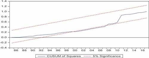
We further estimated the Unrestricted Error Correction Model (UECM) within the framework of the ARDL to capture both the short-run and the long-run relationships among the variables. Only the coefficient of the long-run parameter of real government expenditure is statistically significant. Thus, a 1% change in both government expenditure may lead to approximately 0.1856% in real GDP (see Table 3). The coefficient of the policy dummy in the long-run is insignificant which implies that in the long-run, policy portfolios did not affect the structural relationship between the variables under study. Turning to the short-run dynamics, all the parameters are significant except the real government expenditure. Thus, the lagged error correction term is negative³ and statistically significant implying that shocks to the equilibrium relationship could be restored at a rate of approximately 4% per annum. Furthermore, standard Wald tests on the coefficients were conducted. To this end, the null hypotheses of no Granger Causality from government expenditure to economic growth is not rejected at the 1% level of significance. This implies that in the short-run, public spending does not Granger-cause economic growth and the reverse holds. Model diagnostic are further carried out to check the fitness of the model. To this end, the Jacque-Bera normality test shows that the residuals of the model are not normally distributed. However, the Ramsey RESET test shows that the model is well specified (i.e. we fail to reject the null hypothesis at 1% that the functional form is correctly specified) and the LM test shows that there is no serial correlation in the residuals of the model (see Appendix B). Furthermore, the CUSUM of Squares⁴ graph shows that the mean limit crosses the 5% critical level implying that the coefficients of the parameters of the model are not stable across the time horizon under study (see Appendix C).

Table 3. Long-run and short-run elasticities

Panel A: Long-run elasticities, Dependent Variable, lnYt
Independent variables	Coefficients	Standard error	t-ratio	P-values
C	22.7177	0.5191	43.7598	0.0000
lnGt-1	0.1856	0.0669	2.7750	0.0077^b
Policyt-1	0.4618	1.3048	0.3539	0.7249^b
Panel B: Short-run elasticities Dependent Variable, ∆lnYt
∆lnGt	0.0061	0.0078	0.7835	0.4370
Policy	−0.0684	0.0379	−1.8018	0.0776
ECTt-1	−0.0365	0.0048	−7.5721	0.0000^a

Note: ^{a, b} and ^c indicate significance at 1%, 5% and 10%, respectively.

Furthermore, in an effort to balance the findings of UECM, a non-Granger Causality test by way of the standard Modified Wald test of Toda and Yamamoto (1995) is carried out.

The first step in this process is to appreciate the properties of these data series to determine the maximum order of integration as well as the optimal lag length for the augmented VAR (for the augmented VAR (k + d_max). All the series are integrated at order one ($d_{max}=1$). Moreover, the optimal lag length (see Appendix D) chosen is (k=1)⁵. A standard MWALD test based on the standard asymptotic distribution is carried out on the coefficients of the variables to find out if there is a non-Granger causality or otherwise. To this end, since the p-value (0.0356) is bigger than the significance level of 1%, the null hypothesis of no Granger Causality from public expenditure to real GDP is not rejected. In a similar vein, the null hypothesis of no Granger from economic growth to government expenditure is not rejected (see Table 4). Thus, there is unidirectional Granger causality from economic growth to government expenditure. Therefore, this result refutes the Wagner’s hypothesis that there is a long-run tendency for public expenditure to grow at the backdrop of economic growth. These findings are consistent with that of Ghali (1999) and Ravn et al. (2012). These key findings have significant implications for fiscal space and the economic structure.

Table 4. Granger non-causality tests

Null Hypothesis	Modified Wald statistics	P-value	Decision
lnYt↛lnGt	0.0636	0.9687	Fail to Reject
lnGt↛lnYt	6.6692	0.0356	Reject^b
Diagnostic tests
LM (2)	6.0244 [0.1973]^a
Hetero (1)	31.4263 [0.1419]^a
J-B Normality	17.5878 [0.0015]

Note: Note: ↛ Implies does not cause. ^{a, b} and ^c indicate significance at 1%, 5% and 10%, respectively. LM: Lagrange multiplier test of residual serial correlation. ARCH: autoregressive conditional heteroscedasticity test of residuals. Heteroscedasticity: This is based on the regression of squared residuals on squared fitted values. Normality is based on a test of skewness and kurtosis of residuals. The values in the parenthesis are the p-values.

5. Conclusion and policy implications

This study explores the causal nexus between real public expenditure and real economic growth. The unit root test shows that all the variables are integrated at order one and the Johansen (1991,1995) and Pesaran et al. (2001) cointegration tests show that the variables are cointegrated. Furthermore, the Toda-Yamamoto non-Granger causality method show that there is no Granger causality between economic growth and public expenditure therefore refuting the Wagner’s hypothesis with respect to the Ghanaian economy.

One of the plausible implications of these findings given the assumption that the current trend will continue is that government expenditure will not necessarily translate into economic growth.. It is therefore suggested that the government puts measures in place to streamline government expenditures to ensure fiscal discipline.

Additional information

Funding

The authors received no direct funding for this research.

Notes on contributors

John Gartchie Gatsi

John Gartchie Gatsi is an Associate Professor of Finance at the Department of Finance, School of Business, University of Cape Coast. He has published papers in CogentOA in the area of corporate governance and other peer-reviewed journals.

Michael Owusu Appiah is a Lecturer at the Department of Finance has published papers in peer reviewed in journals in the area of Finance and Energy.

Joseph Addo Gyan is an Assistant to the Prof Gatsi and Dr. Appiah in writing this paper in which he contributed greatly.

Notes

1. http://ghana.opendataforafrica.org/qhvrvi/external-debt-by-country-data-and-charts?country=Ghana.

2. C = Constant and T = Trend.

3. This is the expected right sign.

4. Brown et al. (1975) developed the CUSUM.

5. The optimal lag length of the AVAR is chosen based on the following criteria: Log-Likelihood (LGKL), Likelihood ratio (LR), Hannan-Quinn (HQ), AIC and Schwarz Information Criteria (SIC).

Appendix A.

ARDL bounds testing results for cointegration

Table

Dependent Variable	Function	F- test statistic
Model 1	F (lnY|lnG)	16.8319^a
Model 2	F (lnG|lnY)	9.5333^b
Asymptotic critical values
1%		5%		10%
I (0)	I (1)	I (0)	I (1)	I (0)	I (1)
5.6970	6.9870	4.000	5.0570	3.2700	4.2600

Note: ^{a, b} and ^c denotes significance levels at 1%, 5% and 10%, respectively. Source of critical values: Narayan (2005, p. 1988).

Appendix B.

Table

Model Diagnostics of ARDL	F-Statistics	P-value
LM (3)	1.6934^a	[0.1469]
ARCH (3)	1.4726^a	[0.2232]
J-B Normality	17.5327	[0.0002]
Ramsey’s RESET (2)	5.7165^a	[0.0059]

Note: LM: Lagrange multiplier test of residual serial correlation. ARCH: autoregressive conditional heteroscedasticity test of residuals. Heteroscedasticity: This is based on the regression of squared residuals on squared fitted values. Normality is based on a test of skewness and kurtosis of residuals. ^{a, b} and ^c denotes significance levels at 1%, 5% and 10%, respectively.

Appendix C.

Plots of CUSUM of recursive residuals

Appendix D.

  Lag Selection Criteria for the Augmented VAR and model diagnostics test statistics

Lag	LogL	LR	FPE	AIC	SC	HQ
0	-114.1068	NA	0.671555	5.277580	5.358679	5.307655
1	42.71810	292.2645*	0.000646*	-1.669004*	-1.425706*	-1.578778*
2	46.01567	5.845694	0.000668	-1.637076	-1.231578	-1.486698
3	49.78812	6.344586	0.000678	-1.626733	-1.059036	-1.416204
4	50.85888	1.703475	0.000779	-1.493585	-0.763690	-1.222905
5	53.56845	4.064350	0.000834	-1.434929	-0.542835	-1.104098
6	58.28047	6.639675	0.000820	-1.467294	-0.413000	-1.076311

Note: NA denotes not applicable and * denotes the chosen lag

References

- Agiakloglou, C, & Newbold, P. (1992). Empirical evidence on dickey-fuller-type tests. Journal Of Time Series Analysis, 13(6), 471-12.
- Al-Faris, A. F. (2002). Public expenditure and economic growth in the gulf cooperation council countries. Applied Economics, 34(9), 1187-1193.
- Ansari, M. I, Gordon, D. V, & Akuamoah, C. (1997). Keynes versus wagner: public expenditure and national income for three african countries. Applied Economics, 29(4), 543-550.
- Attari, M. I. J., & Javed, A. Y. (2013). Inflation, economic growth and government expenditure of pakistan: 1980-2010. Procedia Economics and Finance, 5, 58–67.
- Babatunde, M. A. (2011). A bound testing analysis of wagner's law in nigeria: 1970-2006. Applied Economics, 43(21), 2843-2850.
- Bird, R. M. (1971). Wagner's law of expanding state activity. Public Finance = Finances Publiques, 26(1), 1-26.
- Brown, R. L, Durbin, J, & Evans, J. M. (1975). Techniques for testing the constancy of regression relationships over time. journal of the royal statistical society: series b (methodological). 37(2), 149-163.
- Chang, T. (2002). An econometric test of wagner's law for six countries based on cointegration and error-correction modelling techniques. Applied Economics, 34(9), 1157-1169.
- Courakis, A. S, Moura-Roque, F, & Tridimas, G. (1993). Public expenditure growth in greece and portugal: wagner's law and beyond. Applied Economics, 25(1), 125-143.
- Dickey, D. A, & Fuller, W. A. (1979). Distribution of the estimators for autoregressive time series with a unit root. Journal Of The American Statistical Association, 74(366a), 427-431.
- Engle, R. F., & Granger, C. W. J. (1987). Co-integration and error-correction: Representation, estimation and testing. Econometrica, 55, 987–1008. doi:10.2307/1913236
- Gandhi, V. P. (1971). Wagner's law of public expenditure: do recent cross-section studies confirm it?. Public Finance =Finances Publiques, 26(1), 44-56.
- Ghali, K. H. (1999). Government size and economic growth: Evidence from a multivariate cointegration analysis. Applied Economics, 31(8), 975–987. doi:10.1080/000368499323698
- Granger, C. W. (1969). Investigating causal relations by econometric models and cross-spectral methods. Econometrica: Journal of the Econometric Society, 37, 424–438. doi:10.2307/1912791
- Granger, C. W., & Newbold, P. (1974). Spurious regressions in econometrics. Journal of Econometrics, 2(2), 111–120. doi:10.1016/0304-4076(74)90034-7
- Hamdi, H, & Sbia, R. (2013). Dynamic relationships between oil revenues, government spending and economic growth in an oil-dependent economy. Economic Modelling, 35, 118-125.
- Huang, C. J. (2006). Government expenditures in china and taiwan: do they follow wagner's law?. Journal Of Economic Development, 31(2), 139.
- Iniguez-Montiel, A. J. (2010). Government expenditure and income in mexico: keynes versus wagner. Applied Economics Letters, 17(9), 887-893.
- Johansen, S. (1991). Estimation and hypothesis testing of cointegration vectors in Gaussian vector autoregressive models. Econometrica: journal of the Econometric Society, 1551–1580.
- Johansen, S. (1995). Identifying restrictions of linear equations with applications to simultaneous equations and cointegration. Journal Of Econometrics, 69(1), 111–132.
- Johansen, S. (1998). Statistical analysis of cointegration vectors. Journal Of Economic Dynamics and Control, 12(2–3), 231-254.
- Kumar, S, Webber, D. J, & Fargher, S. (2012). Wagner's law revisited: cointegration and causality tests for new zealand. Applied Economics, 44(5), 607-616.
- Kwiatkowski, D, Phillips, P. C, Schmidt, P, & Shin, Y. (1992). Testing the null hypothesis of stationarity against the alternative of a unit root: how sure are we that economic time series have a unit root?. Journal Of Econometrics, 54(1–3), 159-178.
- Loxley, J. (1990). Structural adjustment in Africa: Reflections on Ghana and Zambia. Review of African Political Economy, 17(47), 8–27. doi:10.1080/03056249008703845
- Lyare, S. O, & Lorde, T. (2004). co-integration, causality and wagner's law: tests for selected caribbean countries. Applied Economics Letters, 11(13), 815-825.
- MacKinnon, J. G. (1996). Numerical distribution functions for unit root and cointegration tests. Journal Of Applied Econometrics, 11(6), 601-618.
- Menyah, K, & Wolde-Rufael, Y. (2013). Government expenditure and economic growth: the ethiopian experience, 1950-2007. The Journal Of Developing Areas, 47(1), 263-280.
- Nakibullah, A, & Islam, F. (2007). Effect of government spending on non-oil gdp of bahrain. Journal Of Asian Economics, 18(5), 760-774.
- Narayan, P. K. (2005). The saving and investment nexus for China: Evidence from cointegration tests. Applied Economics, 37(17), 1979–1990. doi:10.1080/00036840500278103
- Narayan, P. K, Nielsen, I, & Smyth, R. (2008). Panel data, cointegration, causality and wagner's law: empirical evidence from chinese provinces. China Economic Review, 19(2), 297-307.
- Narayan, P. K, Prasad, A, & Singh, B. (2008). A test of the wagner's hypothesis for the fiji islands. Applied Economics, 40(21), 2793-2801.
- Narayan, S, Rath, B. N, & Narayan, P. K. (2012). Evidence of wagner's law from indian states. Economic Modelling, 29(5), 1548-1557.
- Oxley, L. (1994). Cointegration, causality and wagner's law: a test for britain 1870-1913. Scottish Journal Of Political Economy, 41(3), 286-298.
- Paparas, D., Richter, C., & Kostakis, I. (2019). The validity of Wagner’s Law in the United Kingdom during the last two centuries. International Economics and Economic Policy, 16(2), 269–291. doi:10.1007/s10368-018-0417-7
- Pesaran, M. H., Shin, Y., & Smith, R. J. (2001). Bounds testing approaches to the analysis of level relationships. Journal of Applied Econometrics, 16(3), 289–326. doi:10.1002/(ISSN)1099-1255
- Phillips, P C, & Perron, P. (1988). Testing for a unit root in time series regression. Biometrika, 75(2), 335–346. doi: 10.1093/biomet/75.2.335
- Ram, R. (1986). Causality between income and government expenditure: a broad international perspective. Public Finance=finances Publiques, 41(3), 393-414.
- Ravn, M. O, Schmitt-Grohe, S, & Uribe, M. (2012). Consumption, government spending, and the real exchange rate. Journal Of Monetary Economics, 59(3), 215-234.
- Samdram, M, Nair, M, & Vaithilingam, S. (2009). Keynes and wagner on government expenditures and economic development: the case of a developing economy. Empirical Economics, 36(3), 697-712.
- Toda, H. Y, & Yamamoto, T. (1995). Statistical inference in vector autoregressions with possibly integrated processes. Journal Of Econometrics, 66(1–2), 225-250. doi:10.1016/0304-4076(94)01616-8
- Wagner, R. E., & Weber, W. E. (1977). Wagner’s law, fiscal institutions, and the growth of government. National Tax Journal, 30,59–68.
- World Bank. 2019. World development indicators. Retrieved from https://data.worldbank.org/country/ghana