Dynamic modeling of systemic risk and firm value: A case of Pakistan

Abstract

The study examines the systemic risk of banking sector in Pakistan and elucidates the factors that exacerbate the systemic risk taking. First, a systemic risk measure ∆CoVaR is applied to analyze the contribution of individual institution to the whole financial system. Secondly, systemic risk and firm value are modeled in static and dynamic frameworks to measure the factors that build systemic risk and firm value. Most importantly, the study highlights the sector level variables munificence, dynamism and concentration are also important in comprehending the risk dynamics along with the much-emphasized firm and country level variables, notably size, political stability, and bank claims. The results imply that the repercussions of excessive risk taking can be ameliorated by increasing liquidity requirements and having a close watch on leverage. Accordingly, monetary policy should be aligned with macro prudential policy to alleviate systemic risk. Furthermore, the Granger causality results indicate that systemic risk engenders idiosyncratic risk and not vice versa, implying regulation of systemic risk can lower the idiosyncratic risk as well. Last but not the least, systemic risk has positive effect on valuation, implying systemic risk cannot be curbed by sheer market discipline and requires external intervention.

Keywords:

• Systemic risk
• ∆CoVaR
• sectoral variables
• bank valuation
• micro and macro prudential regulations

PUBLIC INTEREST STATEMENT

Systemic risk is of concern for economic welfare as systemic financial crisis has the potential to inefficiently lower the supply of credit to the non-financial sector. Financial institutions also accept deposits from public and systemic financial crisis can potentially deprive the depositors from their hard-earned money. Moreover, investors of non-financial sector, employees, and customers can also get useful information about the contagious events that can put the whole system in the crisis. The results divulge how distress of financial institutions affects the financial system and how this distress encompasses other sectors. One of the features of systemic risk is that it can run through the whole economy, and this brings in public as stakeholders. This study can enlighten the public about the risk that can potentially jeopardize the whole economy and how it can be curbed. Consistent with this purview, the study lays down foundation of comprehensive framework to reign in excessive systemic risk taking.

1. Introduction

The instability of inter-connected financial institution is not confined to that institution but is of contagious nature tending to spread through the financial system and causes severe negative macroeconomic shocks. The sub-prime mortgage crises of 2008 highlighted that a shock originating from a single financial institution or country can rapidly extend to other institutions and markets. These spillovers were later identified as a materialization of systemic risk and highlighted the need for a better understanding of this phenomenon.

Despite a large number of published studies, there is no single consensus definition of systemic risk due to difference in the perception of researchers about what constitutes a system and what leads to the buildup of this risk. Nevertheless, Systemic risk has the potential to inefficiently lower the credit supply to whole economy and requires interventions from regulatory authorities to avoid contagion during the periods of market stress (Acharya, 2009; Anginer, Demirguc-Kunt, & Zhu, 2014). The creation of Basel Committee on banking supervision lead to many regulations across the countries but it was the aftermath of subprime crisis that shifted the attention from stand alone to systemic risk. Since then researchers have widely addressed that issue but the sample constitutes of developed economies (Castro & Ferrari, 2014; Soedarmono & Sitorus, 2017) and the literature from developing and emerging economies is scanty (de Mendonça & Da Silva, 2017). This study brings diversity in the literature by providing empirical evidence on systemic and idiosyncratic risk from the financial sector of a developing economy.

The banking sector of Pakistan has shown robust growth in the recent times, and growth of banking sector is also attributed to the buildup of systemic risk (Zedda & Cannas, 2017)¹. Moreover, the financial institutions of Pakistan are important source of financing for other sectors as stock and bond markets are comparatively less developed (Anwar, 2012) making them an important constituent in the network and augments their systemic importance. The stability of financial system can be maintained by identifying systemically important financial institutions and calibrating regulations according to systemic importance of these institutions (Bernal, Gnabo, & Guilmin, 2014). Consistent with this purview, this study measures systemic risk of financial institutions of Pakistan for the first time incorporating weekly returns (losses) data using conditional value at risk approach (∆CoVaR). ∆CoVaR is the contribution of an individual institution to the deficiency of the whole system (Adrian & Brunnermeier, 2016).

Furthermore, the complete dynamics of systemic risk can only be comprehended by examining the factors that build up systemic risk (Kleinow, Horsch, & Molina, 2017). In the like manner, the study investigates the factors that influence the systemic risk taking of financial institutions and how systemic risk affects firm value. Many studies have focused on the determinants of systemic risk in developed economies but literature is scarce in developing and emerging economies (de Mendonça & Da Silva, 2017; Kleinow et al., 2017). Moreover, the literature on firm specific factors is scarce even in developed economies (Iqbal, Strobl, & Vahamaa, 2015) whereas, the sector level variables are nearly neglected apart from concentration. Each sector has its own environment and extant literature outlines the influence of sectoral environment on the decision making of financial institutions and industry effects outperform country effects (Lee & Huang, 2003). Taking the lead from previous studies (Iqbal et al., 2015; Kleinow & Nell, 2015; Strobl, 2016) an empirical model is developed that includes the most common firm and country characteristics of systemic and idiosyncratic risk. Sector level variables are also included in the model. Artificial nested testing procedure results show the statistical model with sector level variables is superior to all the other models, outlining significance of munificence, dynamism, and concentration in comprehension of complete risk dynamics.

In addition to that, Granger causality results divulge systemic risk engenders idiosyncratic risk and not vice versa implying regulation of systemic risk can lead to reduction in idiosyncratic risk. Moreover, the positive impact of systemic risk on firm value reflects that systemic risk cannot be regulated by sheer market discipline and requires external intervention. Besides that, the estimation results further reveal strong persistence of risk and dynamic nature of risk models. Most importantly, the study outlines important relationships and lays down foundation for introducing micro and macro prudential policies.

2. Literature review

2.1. Use of ∆CoVaR as a measure of systemic risk

The systemic risk diagnosis must be correct to introduce adequate regulatory policies. If the systemic risk analysis is not correct, the corresponding regulations will also turnout to be futile. Among the different measures used to gauge systemic risk, conditional value at risk (ΔCoVaR) is one of the most widely used and reliable measures of systemic risk (Castro & Ferrari, 2014; Drakos & Kouretas, 2015)². Adrian and Brunnermeier (2011) introduced ΔCoVaR and define it as the value at risk (VaR) of the system returns conditional on the distress of a financial institution. ΔCoVaR examines the contribution of financial institutions to overall systemic risk, and it can also be used to analyze systemic risk of markets. Moreover, the data required to compute ΔCoVaR is publically available and computations are comparatively simple. In addition to ΔCoVaR, MES (introduced by Acharya, Pedersen, Philippon, & Richardson, 2017) is one of the most widely used measures of systemic risk that gauges the sensitivity of financial institutions to stress of the market. This article attempts to examine the sensitivity of financial system to stress of individual institutions that warrants the use of ΔCoVaR.

Among the studies that apply ΔCoVaR as measure of systemic risk, Stolbov (2017) use ΔCoVaR to investigate systemic risk of 11 developed economies and explicate the role of country level variables in the buildup of systemic risk. Besides that, Andries and Mutu (2016) investigate the impact of corporate governance and regulations on systemic risk (CoVaR) in CEEC. Furthermore, de Mendonça and Da Silva (2017) use ∆CoVaR to identify the determinants of systemic risk in Brazil and divulge liquidity and monetary policy as main drivers of systemic risk. Moreover, Borri, Caccavaio, Di Giorgio, and Sorrentino (2014) apply ∆CoVaR to analyze systemic risk of the banking sector in Italy and report size and leverage as main predictors of systemic risk.

3. Drivers of systemic risk

3.1. Firm level characteristics

The first explanatory variable included in the analysis is size. According to Kleinow and Nell (2015) larger banks might have less idiosyncratic risk because of high level of diversification but that argument holds true only for standalone risk. Conversely, Strobl (2016) argue in favor of negative effect of size on systemic risk. In addition to size, a good part of banking literature suggests positive impact of leverage on systemic risk as high debt makes the bank susceptible to insolvency reducing the ability to absorb the shocks (Bessler, Kurmann, & Nohel, 2015; Brunnermeier, Dong, & Palia, 2012)³.

Another firm level determinant, liquidity is considered to augment the capacity of bank to sustain shocks during the periods of crisis and results in lower level of systemic risk (Brunnermeier et al., 2012; Kleinow et al., 2017; Lin, Sun, & Yu, 2016). To explicate the intensity of revenue side diversification, non-interest income is included in the analysis. In developed economies, it is considered as diversification and construed as a mean of lowering the systemic risk (Bessler et al., 2015; Kleinow & Nell, 2015; Laeven & Levine, 2009). On the other hand, in developing and emerging economies, it is considered as nontraditional risky activity and hence a mean of exacerbating the both types of risk taking (Black, Correa, Huang, & Zhou, 2016; Brunnermeier et al., 2012). Another bank level variable included in the analysis is deposit ratio. According to Strobl (2016), private creditors impose fewer restrictions on the banks, which can result in high-risk taking. Contrary to that Kleinow et al. (2017) espouse that high deposit ratio implies that a large chunk of banks finances comes from private creditors and it reduces systemic risk as private depositors and creditors react slowly to the crisis as compared to the financial institutions.

Literature suggests mixed evidence of the impact of idiosyncratic risk on systemic risk. For instance, Strobl (2016) use granger causality test to analyze the direction of causality between systemic and idiosyncratic risk (stock retrns volatility) and report that systemic risk engenders idiosyncratic risk. Concomitantly, Strobl (2016) argue that increase in firm specific risk makes the firm more vulnerable to collapse thus increasing the systemic risk. These findings are corroborated by Teply and Kvapilikova (2017) who divulge significant positive impact of idiosyncratic risk (VaR) on systemic risk.

3.2. Sector level characteristics

Sector level variables included in the analysis are concentration, munificence, and dynamism. Industry concentration refers to the level of competitiveness with more concentration referring to less competition and vice versa. According to recent research increase in competition can increase the fragility of the financial system resulting in increased level of systemic risk (Beck, Demirguc-Kunt, & Levine, 2006; Jimenez, Lopez, & Saurina, 2013; Kleinow et al., 2017). Another sector level variable, dynamism measures the extent to which a firm’s external environment is stable or unstable (Smith, Chen, & Anderson, 2014). Systemic risk builds up in tranquil times as low volatility in booms entices the managers of financial institutions to take more risk, which eventually results in exacerbation of systemic risk (Adrian & Boyarchenko, 2012; Adrian & Brunnermeier, 2016).

To describe the growth of the sector, munificence is included in the analysis. According to Almazan and Molina (2005), high munificence leads to higher level of opportunities which can eventually augment the financial performance of the organization. Higher growth in the banking sector is attributed to the buildup of systemic risk as lending activities of the banks grow which results in amplification of systemic risk (Zedda & Cannas, 2017). On the other hand, Dell’Ariccia and Marquez (2006) propound that booms are associated with development of banking sector in developing economies.

3.3. Country and regulatory variables

World Bank Worldwide Governance Indicators database provide data on various macro-economic indicators of the countries. Consistent with the previous literature, the first index that is extracted from this database is political stability. A good part of banking literature outlines the negative impact of political stability on systemic risk (Kleinow & Nell, 2015; Uhde & Heimeshoff, 2008). In addition to that, monetary policy is also construed as significant driver of systemic and idiosyncratic risk. Expansionary monetary policy is construed to increase the market value of the banks, which discourages the risk taking (Dell’Ariccia, Laeven, & Marquez, 2014). Another index provided by the World Bank database is claims of the banks on the central government. Bank claims highlight the interrelation between the country and its domestic banks and if domestic banks have high claims on the government, it can substantially increase the systemic risk (Kleinow et al., 2017; Kleinow & Nell, 2015).

3.4. Systemic risk and firm value

Previous research mainly remained focused on identifying systemically important institutions and elucidating the factors that build systemic risk. As far as empirical evidence on impact of systemic risk on firm value is concerned, literature appears to be limited. Recently, Strobl (2016) outline significant positive impact of systemic risk on market value of the firm. Likewise, profitability, deposit ratio, non-interest income to total income, liquidity, concentration along with size and leverage are also discussed as important determinants of firm value (Baek & Bilson, 2015; Saona & Martin, 2016; Strobl, 2016). These determinants are also incorporated as controlled variables in the analysis.

4. Data and methodology

4.1. Sources of data and sample population

There are 35 scheduled banks operating in Pakistan. Out of these banks, 20 are listed at Stock Exchange. The reason behind selecting the listed banks is requirement of stock prices to compute measure of systemic risk. Data were analyzed from 2000 to 2017. The data on firm level variables were extracted from the financial statement analysis of financial sector published by State Bank of Pakistan. The data on country level variables were extracted from Publications of State Bank of Pakistan, Worldwide Governance and Development Indicators, Economic Surveys, and Federal Bureau of Statistics. The sector level variables were manually computed (see Appendix A). Weekly data on share prices of the banks listed at Pakistan Stock Exchange and KSE 100 index were retrieved from Brecorder.com.

4.2. Measurement of ∆ CoVaR

Adrian and Brunnermeier (2016) introduced ∆CoVaR and applied quantile regression as an estimation approach. Adrian and Brunnermeier (2016) defined $CoVa{R}_q^{j/i}$ as the $Va{R}_q^j$ of institution j (or of the financial system) conditional on some event C($R^i$) of institution i. Then $CoVa{R}_q^{j/i}$ is the $q^{th}$ quantile of the conditional probability distribution of returns of j.

(3.1) $\mathrm{P}\left(R^j\le CoVaR{}_q^{j/C{R}^i}|\mathrm{C}\left(R^i\right)\right)$(3.1)

The CoVaR of the financial institution is applied in five stages. The first stage is to assess the returns of institution “i” as a function of lag of state variables as referred by Adrian and Brunnermeier (2016).

(3.2) $R_t^i={\alpha }_q^i+{\gamma }_q^i{M}_{t-1}+{\epsilon }_{qt}^i$(3.2)

This analysis incorporates value from publically available data hence, $R_t^i$ (Return, Losses) are computed as;

$R_t^i=\frac{-\mathrm{\Delta }{R}_t^i}{R_{t-1}^i}$

In Equation (3.2)(3.2) $R_t^i={\alpha }_q^i+{\gamma }_q^i{M}_{t-1}+{\epsilon }_{qt}^i$(3.2) ${\alpha }^i$ is the constant, $M_{t-1}$ is the vector of lag of state variables, and ${\epsilon }_t^i$ is the error term. In the second stage, 1% value at risk of every financial institution is computed. All the insignificant variables in Equation (3.2)(3.2) $R_t^i={\alpha }_q^i+{\gamma }_q^i{M}_{t-1}+{\epsilon }_{qt}^i$(3.2) are eliminated and only significant variables were incorporated in Equation (3.3)(3.3) $V\hat{a}{R}^i={\hat{\alpha }}_q^i+{\hat{\gamma }}_q^i{M}_{t-1}$(3.3) .

(3.3) $V\hat{a}{R}^i={\hat{\alpha }}_q^i+{\hat{\gamma }}_q^i{M}_{t-1}$(3.3)

In Equation (3.3)(3.3) $V\hat{a}{R}^i={\hat{\alpha }}_q^i+{\hat{\gamma }}_q^i{M}_{t-1}$(3.3) ${\hat{\alpha }}^{i}and{\hat{\gamma }}^i$ are estimated from Equation (3.2)(3.2) $R_t^i={\alpha }_q^i+{\gamma }_q^i{M}_{t-1}+{\epsilon }_{qt}^i$(3.2) . In the third step, return of financial system will be computed using Equation (4). Financial system variable represents weekly return (losses) on the portfolio of listed banks included in the analysis and is calculated by generating a value-weighted index of these banks.

(3.4) $R_t^{System}={\alpha }_q^{System\left|i\right.}+{\beta }_q^{System\left|i\right.}{R}_t^i+{\gamma }_q^{System\left|i\right.}{M}_{t-1}+{\epsilon }_{qt}^{System\left|i\right.}$(3.4)

In the fourth stage, CoVaR is calculated by computing value at risk (1%) from Equation (3.3)(3.3) $V\hat{a}{R}^i={\hat{\alpha }}_q^i+{\hat{\gamma }}_q^i{M}_{t-1}$(3.3) and all the significant state variables from Equation (3.4)(3.4) $R_t^{System}={\alpha }_q^{System\left|i\right.}+{\beta }_q^{System\left|i\right.}{R}_t^i+{\gamma }_q^{System\left|i\right.}{M}_{t-1}+{\epsilon }_{qt}^{System\left|i\right.}$(3.4) in Equation (3.5)(3.5) $CoVa{R}_t^i={\hat{\alpha }}^{System\left|i\right.}+{\hat{\beta }}_q^{System\left|i\right.}Va{R}_{qt}^i+{\hat{\gamma }}^{System\left|i\right.}{M}_{t-1}.$(3.5) .

(3.5) $CoVa{R}_t^i={\hat{\alpha }}^{System\left|i\right.}+{\hat{\beta }}_q^{System\left|i\right.}Va{R}_{qt}^i+{\hat{\gamma }}^{System\left|i\right.}{M}_{t-1}.$(3.5)

In the last stage, ∆CoVaR is estimated. It is the difference between CoVaR of the system at 1 and 50% quantile. The calculation of 50% CoVaR is similar to that of 1% quantile. Consistent with de Mendonça and Da Silva (2017), geometric mean of ∆CoVaR is taken to perform the estimations.

(3.6) $\begin{array}{rl}& \mathrm{\Delta }Co\hat{V}a{R}_{99t}^i\left(q\right)=Co\hat{V}aR\left(1\mathrm{\%}\right)-Co\hat{V}a{R}_t^i(50\mathrm{\%})\\ & ={\hat{\beta }}_q^{Systemi|i}\left(Va{R}_{q,t}^i-Va{R}_{50,t}^i\right)\end{array}$(3.6)

4.3. State variables

According to Adrian and Brunnermeier (2016), state variables are used to condition the mean and variability of risk measures and should not be construed as systemic risk factors. The change in three-month Treasury bill rate is used as change captures the extreme returns better than level. The weekly market return is calculated from KSE100 Index. The change in slope of yield curve is calculated by taking the difference between long-term bond and Treasury bill rate. The change in credit spread is difference between Moody’s Baa rated bonds and ten-year treasury bond rate. Equity volatility is calculated as the 22 day rolling standard deviation of the KSE100 index equity market returns. Data on inflation are monthly, hence it is collapsed to weekly to commensurate with other state variables. All the variables are set at weekly frequency.

4.3.1. Estimation of systemic risk, idiosyncratic risk, and firm value

The study firstly applies fixed effect regression based on Hausman specification. According to Pikas and Lee (2003) fixed effect and OLS regression results are vulnerable to upward and downward bias, respectively. The application of GMM eliminates that problem and results in efficient estimates. In addition to that, Arellano and Bover (1995) propound that endogenity in the model can be avoided by taking the first difference of data and incorporating the lag of endogenous variables as instruments. Later on Blundell and Bond (1998) state that Difference GMM introduces bias in small and large samples and recommend the use of System GMM.

According to Roodman (2009), results of small samples are vulnerable to bias due to large number of instruments in System GMM. This study ensures to keep the number of instruments below the number of groups to ensure too many instruments don’t over fit the sample. In addition to that, the results of GMM are reliable in the absence of serial correlation of order 2 or beyond. First and second order test of correlation are performed in the study. Furthermore, Sargan and J-test are performed to analyze the exogeneity of the instruments used.

(3.7) $\begin{array}{rl}& \mathrm{\Delta }Sytemi{c}_{it}={\beta }_0+{\beta }_{1}Systemi{c}_{i,t-1}+{\beta }_{2}Idi{o}_{i,t}+{\beta }_{3}SIZ{E}_{i,t}+{\beta }_{4}LE{V}_{i,t}+{\beta }_{5}IncomeDive{r}_{i,t}\\ & +{\beta }_{6}Liquidit{y}_{i,t}+{\beta }_{7}MUNI{F}_t+{\beta }_{8}DYNA{M}_t+{\beta }_{9}CONCEN{T}_t+{\beta }_{11}Claim{s}_t\\ & +{\beta }_{10}POLITSTA{B}_t+{\beta }_{12}Monetar{y}_t+{\epsilon }_{it}\end{array}$(3.7)

Systemic risk is the dependent variable in the model and idiosyncratic risk is residual volatility of stock returns from market model. The complete hierarchy of variables is incorporated in the study and artificial nested testing procedure is performed to examine as if complete hierarchy augments the forecasting ability or expose the model to redundancy. If simple model contributes more information then it should be preferred on complicated model. The preferred model is selected on the basis of F-test⁴. The formulation and empirical evidence on independent variables are provided in Appendix A, Table 10.

(3.8) $\begin{array}{rl}& \mathrm{\Delta }tobin{Q}_{it}={\beta }_0+{\beta }_{1}tobin{Q}_{i,t-1}+{\beta }_{2}SystemicRis{k}_{i,t}+{\beta }_{3}IDIOSYNRis{k}_{i,t}+{\beta }_{4}SIZ{E}_{i,t.}\\ & +{\beta }_{5}LE{V}_{i,t}+{\beta }_{6}LIQUIDIT{Y}_{i,t}+{\beta }_{7}Profitabilit{y}_{i,t}+{\beta }_{8}IncomeDive{r}_{i,t}\\ & +{\beta }_{9}DEPOSI{T}_{i,t}+{\beta }_{10}CONCEN{T}_t+{\epsilon }_{it}\end{array}$(3.8)

∆ tobinQ is the value of the firm. The formulation and empirical evidence on independent variables is provided in Appendix A, Table 10.

Table 10. Variable formulation and empirical evidence

Variable	Measurements & Source	Empirical Evidence
Bank Level Determinants
Size	$Logarithm$ $ofTotalAssets$ State Bank of Pakistan	Kleinow and Nell (2015), Strobl (2016), Kleinow et al. (2017)
Leverage	$\frac{Debt}{TotalAssets}$ State Bank of Pakistan	Strobl (2016), Black et al. (2016), Andries and Mutu (2016)
Profitability	Return on Equity State Bank of Pakistan	Black et al. (2016), de Mendonça and Da Silva (2017)
Liquidity	$\frac{\mathrm{c}\mathrm{a}\mathrm{s}\mathrm{h}\mathrm{f}\mathrm{l}\mathrm{o}\mathrm{w}\mathrm{f}\mathrm{r}\mathrm{o}\mathrm{m}\mathrm{o}\mathrm{p}\mathrm{e}\mathrm{r}\mathrm{a}\mathrm{t}\mathrm{i}\mathrm{o}\mathrm{n}\mathrm{s}}{\mathrm{t}\mathrm{o}\mathrm{t}\mathrm{a}\mathrm{l}\mathrm{l}\mathrm{i}\mathrm{a}\mathrm{b}\mathrm{i}\mathrm{l}\mathrm{i}\mathrm{t}\mathrm{i}\mathrm{e}\mathrm{s}}$ State bank of Pakistan	Lin et al. (2016), de Mendonça and Da Silva (2017), Soedarmono and Sitorus (2017), Black et al. (2016)
Non- Interest Income	$\frac{Non-Interestincome}{TotalinterstIncome}$ State Bank of Pakistan	Kleinow et al. (2017),Strobl (2016)
Deposit Ratio	$\frac{Deposit}{TotalAssets}$ State Bank of Pakistan	Zedda and Cannas (2017), de Mendonça and Da Silva (2017)
Idiosyncratic Risk	$R_{it}={\alpha }_{it}+\beta R_{M,t}$+${\epsilon }_{it}$ $R_{M,t}$ denotes KSE 100 index return. Standard deviation of ${\epsilon }_{it}$ explains the idiosyncratic volatility	Strobl (2016).
Firm Value	$tobinQ=\frac{MarketValueofequity+BookValueofDebt}{TotalAssets}$	Soedarmono and Sitorus (2017), Strobl, 2016)
Sector Level
Munificence	1. Regressing time against the Revenues of banking sector over the period of study and 2. Taking the ratio of the regression slope coefficient to the mean value of revenues over the same period. (Computed by Authors)	Boyd (1995), Kayo and Kimura (2011)
Dynamism	Standard error of munificent slope coefficient divided by the mean value of revenues over the same period. (Computed by Authors)	Boyd (1995), Kayo and Kimura (2011)
Concentration	HHI is the sum of the squares of the market shares (assets) of each bank in the financial system. (Computed by Authors)	Anginer et al. (2014)
Country level
Political Stability	Index of instability of Democracy extracted from Worldwide Governance Indicators.	Kleinow &Nell(2015), Kleinow et al. (2017)
Bank Claim	Banks’ claims on central government as a percentage of GDP include loans to central government institutions net of deposits.(WDI)	Kleinow &Nell (2015), Kleinow et al. (2017)
Monetary Policy	Monetary policy Interest Rate	de Mendonça and Da Silva (2017), Gang and Qian (2015)

Note: The table provides definition and data sources of Firm, Sector and Country level variables.

4.4. Results and interpretation

Table 1 shows the summary statistics of the state variables included in the analysis. The data are set at weekly frequency. The data on inflation are collapsed from monthly to weekly to set the frequency equivalent with other state variables. Term spread shows difference between long- term and short-term treasury rate, and that difference seems to be sizeable. Change in yield of T-bill is not high showing that short-term risk free rates are not volatile. The weekly market returns are also encouraging despite the fact they also include crisis time period. Rolling standard deviation of stock returns is also high showing the volatility of returns.

Table 1. Descriptive statistics

Variable	Obs	Mean	Std. Dev.	Min	Max
Term Spread	911	1.4624	1.2417	−3.2191	4.3208
Change in T-bill	911	0.0032	0.3207	−3.7503	2.6294
Market Return	911	0.3590	3.0743	−18.2103	11.5575
Rolling SD	911	0.6306	0.9811	0.0104	5.1289
Inflation	911	2.0464	0.9930	0.3212	4.7307
Change Spread	911	−5.0045	2.1590	− 8.6500	0.3200

Note: The table shows weekly statistics of state variables incorporated for the measurement of $\mathrm{\Delta }Co\hat{V}a{R}_{99t}^{System}$.

Table 2 shows of 1 and 50% quantile regression results of lag of state variables on stock returns. Results imply that state variables influence stock returns differently when different quantiles are used. Apart from these results, calculations are performed individually for each bank to identify systemically import financial institutions.

Table 2. Quantile regression with stock return (Losses) and system return (Losses) as dependent variable

	Quantile 0.01		Quantile 0.50
	$R_t^i$	$R_t^{System}$	$R_t^i$	$R_t^{System}$
Market Return	0.6109*** (3.60)	0.3956*** (8.26)	0.8769***(62.46)	0.6524***(7.13)
Term Spread	0.1361 (0.39)	−0.0408 (0.77)	0.0479* (1.66)	0.0736***(4.20)
Change in t-bill	−2.5736 (−1.43)	−1.9162*** (−9.73)	−0.3514*** (−2.95)	−0.2915***(−5.19)
Rolling SD	−1.5238***(−5.54)	−1.6170*** (−6.74)	−0.0164 (−0.71)	0.0936***(4.90)
Inflation	−0.9142***(−2.64)	−0.8377*** (−7.82)	0.0344 (1.27)	−0.0552** (−2.35)
Change Spread	−1.1861 (−0.91)	−0.4062 ***(−5.85)	0.0346* (1.93)	0.0023 (0.28)
$R_t^i$	____	0.4122*** (3,71)	____	0.2417***(4.54)
Constant	−8.7142***(−7.14)	−2.7848*** (−3.28)	−0.4871***(−4.59)	−0.1469***(−2.63)
Number of obs	14,728	14,728	14,728	14,728
Pseudo R2	0.4541	0.6118	0.3519	0.4011

Note: Table reports the results of 1 and 50% quantile regression results with return of individual financial institution as dependent variable. (*), (**) and (***) shows significance at 1, 5, and 10%, respectively. T-values are shown in parenthesis. Quantile regression shows pseudo R2 instead of adjusted R2.

Table 3 shows the summary statistics of systemic risk measures. The values clearly indicate that $\mathrm{\Delta }CoVa{R}_{99,t}^i$ is higher than $\mathrm{\Delta }CoVa{R}_{95,t}^i$ implying that the former explains extreme events better than the latter as shown in Figure 1.

Table 3. Descriptive statistics of weekly results (in %)

Variable	Obs	Mean	Std. Dev.	Min	Max
$Va{R}_{95,t}^i$	14,728	−8.059	7.105	−51.457	−2.257
$Va{R}_{99,t}^i$	14,728	−12.51	13.214	−84.890	−3.631
$\mathrm{\Delta }CoVa{R}_{99,t}^i$	14,728	−1.326	1.562	−6.910	−0.183
$\mathrm{\Delta }CoVa{R}_{95,t}^i$	14,728	−0.805	0.595	−4.031	−0.086
$Va{R}_{99,t}^{System}$	907	−5.175	3.499	−32.726	−2.185

Note: The table shows weekly statistics of risk measures along with respective mean and standard deviation. All the values are shown in weekly percentage points.

Weekly ∆CoVaR is shown in absolute values. MCB has highest systemic risk contribution followed by UBL, Habib Bank, NBP and Allied Bank. MCB is the largest bank of Pakistan with current market capitalization of 225.75 billion rupees. UBL is the third largest bank of Pakistan with market capitalization of 177.51 billion rupees and Habib Bank has market capitalization of 209.03 billion rupees making it the second largest bank of Pakistan. The results indicate that size and connectivity both matter in making an institution systemically important.

Figure 1 shows $\mathrm{\Delta }CoVa{R}_{99,t}^i$ average ∆CoVaR of banking sector from 2000 to 2017. Figure 1 divulges that ∆CoVaR experienced an exorbitant increase in 2008 and 2009. The increase in systemic risk is attributed to the volatile situation in the country as political instability and terrorism hit the country hard during that time.

Figure 1. Average CoVaR.

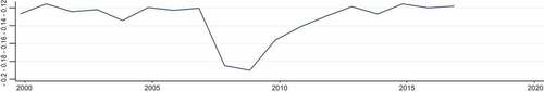
Table 5 shows descriptive statistics of dependent and independent variables incorporated in the study. The data set consists of 20 banks ranging across 18 years. The frequency of data is annual. Mean value of idiosyncratic risk is 2.1710. Leverage is high with mean value of 0.7952 and high mean of deposit ratio confirms that a large chunk of the bank finances comes from private creditors.

Table 4. Systemic importance of financial institutions with respect to $\mathrm{\Delta }CoVa{R}_{99}^i$. The ranking of systemically important financial institutions using∆ CoVaR

Rank	Institution	Average Weekly ∆CoVaR
1	Muslim Commercial Bank (MCBL)	−0.0355
2	United Bank Limited(UBL)	−0.0312
3	Habib Bank Limited (HBL)	−0.0299
4	National Bank Limited (NBPL)	−0.0246
5	Allied Bank Limited (ABL)	−0.0235
6	Meezan Bank Limited	−0.0187
7	Bank Al-Habib Limited	−0.0151
8	Bank ALfalah Limited	−0.0146
9	Bank of Punjab Limited	−0.0117
10	Habib Metro Bank Limited	−0.0098
11	Faysal Bank Limited	−0.0089
12	Standard Chartered Bank Limited	−0.0084
13	Askari Bank Limited	−0.0072
14	Bank of Khyber Limited	−0.0050
15	Soneri Bank Limited	−0.0048
16	BankIslami Pakistan Limited	−0.0044
17	Silk Bank Limited	−0.0042
18	Samba Bank Limited	−0.0039
19	JS Bank Limited	−0.0036
20	Summit Bank Limited	−0.0027

Table 5. Descriptive statistics

Variable	Mean	Std. Dev.	Min	Max
Firm
Idiosyncratic	2.1710	1.0446	1.0791	6.0126
Size	8.1349	5.4611	6.5417	9.4082
Non-Interest	0.1981	0.1025	0.0074	0.3762
Liquidity	0.0671	0.0906	−0.3158	0.2722
Leverage	0.7952	0.9546	0.6339	0.8698
Deposit Ratio	0.7539	0.8612	0.4411	0.8954
Sector
Munificence	0.1014	0.0911	−0.0131	0.2267
Concentration	971.3164	103.1475	852.5903	1525.91
Dynamism	0.0296	0.0133	0.0008	0.0614
Country
Political	−2.3914	0.3491	−2.8100	−1.5831
Claims	0.2161	0.7008	0.1141	0.3166
Monetary Interest	0.0925	0.0263	0.0575	0.1447

Note: The table presents descriptive statistics for bank, sector and country specific financial data used in the panel regressions. Bank-specific data are taken from the databases of State Bank of Pakistan. Sector level variables are computed by authors. Political stability and Bank claims are provided by World Wide Governance and development indicators.

Table 6 shows the result of correlation among key variables. The highest correlation is between systemic risk and negative correlation with idiosyncratic risk. Table 7 and Table 8 shows result of Granger causality. In order to select the lag length AIC (Akaike information criterion), SC(Schwarz information criterion), HQ (Hannan-Quinn information criterion) values are used and all the criteria recommend the use of lag 1. The results show that systemic risk causes idiosyncratic risk whereas idiosyncratic risk does not cause systemic risk. The results are consistent with the findings of Strobl (2016) that systemic risk engenders idiosyncratic risk and not vice versa.

Table 6. Correlation matrix

Systemic	IDIO	Size	LEV	Non-Int	LIQ	Deposit	MUN	CONC	DYNA	Political Claims	Monetary
Systemic	1.0000
Idiosyncratic	0.1087	1.0000
Size	0.3282	−0.2430	1.0000
LEV	0.1514	0.2949	0.2597	1.0000
Non-Int	0.0905	0.0568	0.0257	0.1970	1.0000
LIQ	− 0.0622	−0.0983	0.3921	−0.1182	−0.0783	1.0000
Deposit	−0.0066	−0.1871	0.3871	0.6179	0.1781	0.1116	1.0000
MUN	−0.2107	−0.4988	0.4905	0.4576	−0.1907	−0.0359	0.1359	1.0000
CONC	−0.0296	−0.1376	0.4406	0.0171	0.2107	−0.1164	0.0853	0.0802	1.0000
DYNA	−0.1207	0.5508	−0.0812	−0.0469	0.0834	−0.1476	−0.0463 -	0.5132	−0.5438	1.0000
Political	−0.1807	−0.3510	0.1052	0.0214	−0.0261	−0.1442	0.0390	0.2436	0.1507	−0.1152	1.0000
Claims	0.0513	−0.3184	0.1435	0.0766	−0.0499	0.0029	0.0219	0.0794	−0.3911	0.1813	−0.4256	1.0000
Monetary	0.1318	0.2333	−0.2241	−0.0396	−0.0280	−0.0294	0.1558	−0.5124	0.2072	0.3210	0.1944	−0.1076	1.000

Table 7. Systemic risk granger-cause idiosyncratic risk

W-bar	=	7.2179
Z-bar	=	16.8365 (p = (0.0000)
Z-bar tilde	=	6.3753 (p = 0.0000)

Note: The table reports the statistics Dumitrescu and Hurlin (2012) Granger non-causality test results.

The null hypothesis is ∆CoVaR does not Granger cause idiosyncratic risk.

4.4.1. Estimation of systemic risk & firm value

The study includes hierarchy of variables i.e. firm, sector and country level and artificial nested testing procedure reflects that unrestricted model with complete hierarchy is statistically better than all the restricted models (see Appendix B, Table 11). Systemic risk is estimated using fixed effect, one-step SGMM and two-step SGMM, whereas firm value is estimated using random effect regression. The diagnostic and post estimation tests are presented in the appendix (see Appendix C, Table 12). The tests include Hausman specification, Woodridge test of autocorrelation and Pasaran’s test of cross sectional dependence. The post estimation results of SGMM shows that the null hypothesis of both Sargan tests and J-stat cannot be rejected implying the exogeneity of instruments. Secondly, AR (2) results also confirm the absence of second order autocorrelation. Size has positive impact on systemic (Kleinow & Nell, 2015), and the coefficient is significant in all the models. Leverage exacerbates systemic risk (Bessler et al., 2015) implying that higher debts contribute to the fragility of the system. Increase in liquidity reduces systemic risk (Lin et al., 2016) whereas, non-interest income is insignificant in explaining any variation in systemic risk. Sector level variable, munificence decreases systemic risk (Dell’Ariccia et al., 2014).

This also confirms that growth of banking sector is attributed to development of banking sector and not to systemic risk in developing economy. Environment dynamism has negative influence on systemic risk (Adrian & Boyarchenko, 2012) but its economic significance is very weak. High concentration reduces systemic risk (Kleinow et al., 2017) implying that competition increases the fragility of financial system in the developing economy.

Furthermore, the country level variable political stability has negative impact on systemic (Kleinow et al., 2017) and the same holds true for expansionary monetary policy (de Mendonça & Da Silva, 2017). The results confirm that monetary tightening can put the individual institution and whole financial system in jeopardy. Increase in bank claims lead to build up of systemic risk (Kleinow et al., 2017).

As far as firm value is concerned, Table 9 shows that systemic risk has positive on firm value (Strobl, 2016). The coefficient of lagged value of systemic risk is significant in both models of SGMM. The positive values of lag of systemic risk in both the models imply persistence of risk and similar results are observed by previous studies (de Mendonça & Da Silva, 2017; Soedarmono & Sitorus, 2017).

6. Conclusion

This study examines systemic risk for the economy of Pakistan using ∆CoVaR methodology and highlights systemically important financial institutions of Pakistan. Most importantly, systemically important banks (MCB, UBL, HBL, NBP, and ABL) should be scrutinized more than other banks and the changing impact of firm, sector, and country level variables should be consistently perused by regulatory authorities. The study outlines important relationships and lays down foundation for introducing micro and macro prudential policies. For instance, leverage increases systemic risk and needs proper monitoring by regulatory authorities as banks get large amount of loans during stable times that can wreak havoc during the crisis as it happened in 2008–2009. Accordingly, the State Bank of Pakistan should also introduce higher liquidity requirements as results point out increased liquidity leads to lower level of systemic risk. In the like manner, monetary policy and prudential regulation policy should also be aligned as contractionary monetary policy results in higher level of systemic volatility.

Furthermore, the findings of the study highlight that systemic risk in Pakistan engenders idiosyncratic risk and not the other way around. This implies regulation of the systemic risk can effectively lower the idiosyncratic risk as well. In addition to that, the positive effect of systemic risk on firm value call attention to the fact that systemic risk would never be a problem for company management, requiring interventions from regulatory authorities to reign in excessive systemic risk taking. The study also highlights negative effect of high concentration on systemic risk implying high competition increases the fragility of system. To epitomize, the stability of financial system is very important for the sound working of whole economy and the fragility of system can be avoided by examining risk exposure of financial institutions and introducing timely micro and macro prudential policies including Pigovian tax.

Additional information

Funding

The authors received no direct funding for this research.

Notes on contributors

Hasan Hanif

Hasan Hanif is a lecturer at Air University Islamabad and supervising research projects of MBA and MS students. Moreover, he has many research publications in HEC recognized research journals to his credit. His area of interest is risk management.

Muhammad Naveed

Dr. Muhammad Naveed is an associate professor at SZABIST Islamabad and supervising research work of MS and PhD students. He has many research publications in ESCI and HEC recognized journals and on dividend policy and risk management to his credit.

Mobeen Ur Rehman

Dr. Mobeen ur Rehman is an assistant professor at SZABIST Islamabad and supervising research work of MS and PhD students. He has research publications in Impact factor, ESCI and HEC recognized Journals to his credit. His cumulative Impact Factor is 38.75.

Notes

1. According to the report of State Bank of Pakistan, the total assets of banking sector increased from PKR 6,516 billion to PKR 15,134 billion, rise in deposits from PKR 4,786 billion to PKR 11,092 billion, increase in lending from PKR 3,240 billion to PKR 5,025 billion and rapid surge in investments from PKR 1,737 billion to PKR 7,625 billion.

2. For application of ∆CoVaR in emerging economy see de Mendonça and Da Silva (2017).

3. For further insight on leverage and risk taking, see (Strobl, 2016).

4. See Appendix C, Table 12 for all the restricted combinations of firm, sector and country level variables along with results of F-test.

Appendix A

Table 8. Idiosyncratic risk granger-cause systemic risk

W-bar	=	2.4219
Z-bar	=	1.1961 (p = .2410)
Z-bar tilde	=	−0.1512 (p = .8941)

Table 9. Estimation of firm value

tobinQ	R.E	SGMM1	SGMM2
$tobin{Q}_{t-1}$		0.993 (0.777)	0.225** (0.661)
Systemic Risk	0.174* (0.099)	0.308 (0.218)	0.270* (0.149)
IDIO	−1.451* (0.799)	−0.201** (0.093)	−0.183* (0.102)
Size	0.431*** (0.079)	0.282** (0.134)	0.141* (0.077)
Leverage	−0.310***(0.059)	−0.016* (0.007)	−0.017** (0.006)
Profitability	0.040 (0.063)	0.030** (0.012)	0.022 (0.284)
Non-Interest	−0.103 (0.079)	−0.346 (0.443)	−0.483** (0.235)
Liquidity	0.023 (0.029)	0.146** (0.053)	0.087* (0.044)
Deposit Ratio	0.188 (0.230)	0.091 (0.125)	0.142 (0.117)
Concentration	0.001 (0.002)	0. 0002 (0.0002)	0.004 (0.039)
Constant	1.645***(0.311)	1.138* (0.568)	0.655** (0.300)
Num of obs	309	289	289
$Adj.R{ }^2$	0.4120
F-stat(P-value)	65.72(0.00)	89.99(0.000)	116.43 (0.00)
N.Ins/N.Groups		(0.80)	(0.80)
J-stat(p-value)			12.63(0.404)
Sargan(p-value)		7.53(0.247)	14.14(0.285)
AR(1)p-value		−1.71(0.086)	−2.04(0.045)
AR(2)p-value		0.63(0.547)	0.94 (0.386)

Note: (*), (**) and (***) shows significance at 1, 5, and 10%, respectively. Standard errors are shown in parenthesis. Heteroskedasticity-robust Huber-White standard errors are used AR (1) and AR (2) present results of first and second order correlation in first differenced results. Sargan and J-stat show if instruments are exogenous. J-stat is reported by stata in one-step, resultantly only Sargan stat is reported.

Appendix B

Table 11. Selection of preferred model (Artificial nested testing procedure)

ATNP	Firm	Firm & Sector	Firm & Country	Sector & Country
Systemic risk	F = 22.40	F = 20.35	F = 3.453	F = 74.81
	p = 0.0000	p = 0.0000	p = 0.0173	p = 0.0173

Note: Table A.5 shows F-value and probability of artificial nested testing procedure results. All the restricted combinations are compared with unrestricted model. The null hypothesis is that restricted model is statistically better than unrestricted model. The probability of F-test is 0.000 in all the cases that rejects the null hypothesis that restricted model is better than unrestricted model.

Appendix C

Table 12. Diagnostics and post estimation of fixed effect regression

Test/ Diagnostic	Systemic Risk	Firm Value
Hausman Specification	chi2 = 88.35	chi2 = 7.18
	p = 0.0000	p = 0.6118
Wooldridge test for autocorrelation in panel data	F = 1.914	F = 1.0490
	p = 0.1164	p = 0.3219
Pesaran’s test of cross sectional dependence	Stat = 1.2791
	p = 0.2166
Breusch and Pagan test for Random Effects		Chi-squared = 295.0
		p = 0.000
t-test for significance of sector level variables	F = 3.46
	p = 0.0169

Note: The table provides tests for fixed/random effect regression. Hausman Specification shows application of fixed effect and Wooldridge test rejects the presence of serial correlation. Pesaran Test also rejects cross sectional dependence. Heteroskedasticity-robust Huber-White standard errors are used. T-test shows the significance of sector level variables and validate the inclusion of sector level variables in the model.

References

- Acharya, V. (2009). A theory of systemic risk & design of prudential bank regulations. Journal of Financial Stability, 5(3), 224–17. doi:10.1016/j.jfs.2009.02.001
- Acharya, V. V., Pedersen, L. H., Philippon, T., & Richardson, M. (2017). Measuring systemic risk. Review of Financial Studies, 30, 2–47. doi:10.1093/rfs/hhw088
- Adrian, T., & Boyarchenko, N. (2012). Intermediary leverage cycles & financial stability, FRB of New York Staff Report, 567.
- Adrian, T., & Brunnermeier, M. (2016). CoVaR. American Economic Review, 106(7), 1705–1741. doi:10.1257/aer.20120555
- Adrian, T., & Brunnermeier, M. K. (2011). CoVaR, NBER Working Paper 17454, Cambridge, MA: National Bureau of Economic Research, Inc.
- Almazan, A., & Molina, C. (2005). Intra-industry capital structure dispersion. Journal of Economics & Management Strategy, 14(3), 263–297. doi:10.1111/j.1530-9134.2005.00042.x
- Andries, A. M., & Mutu, S. (2016). Systemic risk, corporate governance & regulation of banks across emerging countries. Economics Letters. doi:10.1016/j.econlet.2016.04.0
- Anginer, D., Demirguc-Kunt, A., & Zhu, M. (2014). How does competition affect bank systemic risk? Journal of Financial Intermediation, 23(1), 1–26. doi:10.1016/j.jfi.2013.11.001
- Anwar, Y. (2012). Long term debt financing - issues & challenges for Pakistan. Paper presented at Institute of Business Management, Karachi, Pakistan.
- Arellano, M., & Bover, D. (1995). Another look at the instrumental variable estimation of error component models. Journal of Econometrics, 68, 29–51. doi:10.1016/0304-4076(94)01642-D
- Baek, S., & Bilson, J. O. (2015). Size & value risk in financial firms. Journal of Banking & Finance, 55(2), 295–326. doi:10.1016/j.jbankfin.2014.02.011
- Beck, T., Demirguc-Kunt, A., & Levine, R. (2006). Bank concentration, competition, & crises: First results. Journal of Banking & Finance, 30(5), 1581–1603. doi:10.1016/j.jbankfin.2005.05.010
- Bernal, O., Gnabo, J., & Guilmin, G. (2014). Assessing the contribution of banks, insurance and other financial services to systemic risk. Journal of Banking and Finance, 47(10), 270–287. doi:10.1016/j.jbankfin.2014.05.030
- Bessler, W., Kurmann, P., & Nohel, T. (2015). Time-varying systematic & idiosyncratic risk exposures of US bank holding companies. Journal of International Financial Markets, Institutions & Money, 35, 45–68. doi:10.1016/j.intfin.2014.11.009
- Black, L., Correa, R., Huang, X., & Zhou, H. (2016). The systemic risk of european banks during the financial & sovereign debt crises. Journal of Banking & Finance. doi:10.1016/j.jbankfin.2015.09.007
- Blundell, R., & Bond, S. (1998). Initial conditions & moment restrictions in dynamic panel data models. Journal of Econometrics, 87, 115–143. doi:10.1016/S0304-4076(98)00009-8
- Borri, N., Caccavaio, M., Di Giorgio, G., & Sorrentino, A. M. (2014). Systemic risk in the Italian banking industry. Economic Notes, 43(1), 21–38. doi:10.1111/ecno.v43.1
- Boyd, B. K. (1995). CEO duality & firm performance: a contingency model. Strategic Management Journal, 16, 301–312. doi:10.1002/(ISSN)1097-0266
- Brunnermeier, M. K., Dong, G., & Palia, D. (2012). Banks’ non-interest income & systemic risk. Working Paper, Princeton University, Princeton, New Jersy.
- Castro, C., & Ferrari, S. (2014). Measuring and testing for the systemically important financial institutions. Journal of Empirical Finance, 25(C), 1–14. doi:10.1016/j.jempfin.2013.10.009
- de Mendonça, H., . F., & Da Silva, R. B. (2017). Effect of banking & macroeconomic variables on systemic risk: An application of ΔCOVAR for an emerging economy. North American Journal of Economics & Finance. doi:10.1016/j.najef.2017.10.011
- Dell’Ariccia, G., Laeven, L., & Marquez, R. (2014). Real interest rates, leverage, & bank risk-taking. Journal of Economic Theory, 149(1), 65–99. doi:10.1016/j.jet.2013.06.002
- Dell’Ariccia, G., & Marquez, R. (2006). Lending booms & lending standards. Journal of Finance, 61(5), 2511–2546. doi:10.1111/j.1540-6261.2006.01065.x
- Drakos, A. A., & Kouretas, G. P. (2015). Bank ownership, financial segments and the measurement of systemic risk: An application of CoVaR. International Review of Economics and Finance, 40(C), 127–140. doi:10.1016/j.iref.2015.02.010
- Dumitrescu, E., . I., & Hurlin, C. (2012). Testing for Granger non-causality in heterogeneous panels. Economic Modelling, 29(4), 1450–1460. doi:10.1016/j.econmod.2012.02.014
- Gang, J., & Qian, Z. (2015). China’s monitory policy & systemic risk. Emerging Markets Finance & Trade, 51, 701–713. doi:10.1080/1540496X.2015.1039895
- Iqbal, J., Strobl, S., & Vahamaa, S. (2015). Corporate governance & the systemic risk of financial institutions. Journal of Economics & Business, 82(1), 42–61. doi:10.1016/j.jeconbus.2015.06.001
- Jimenez, G., Lopez, J. A., & Saurina, J. (2013). How does competition affect bank risk-taking? Journal of Financial Stability, 9(2), 185–195. doi:10.1016/j.jfs.2013.02.004
- Kayo, E., & Kimura, H. (2011). Hierarchical determinants of capital structure. Journal of Banking & Finance, 35(2), 358–371. doi:10.1016/j.jbankfin.2010.08.015
- Kleinow, J., Horsch, A., & Molina, M. G. (2017). Factors driving systemic risk of banks in Latin America. Journal of Economics & Finance, 41, 211–234. doi:10.1007/s12197-015-9341-7
- Kleinow, J., & Nell, T. (2015). Determinants of systemically important banks: the case of Europe. Journal of Financial Economic Policy, 7(4), 446–476. doi:10.1108/JFEP-07-2015-0042
- Laeven, L., & Levine, R. (2009). Bank governance, regulation & risk taking. Journal of Financial Economics, 93(2), 259–275. doi:10.1016/j.jfineco.2008.09.003
- Lee, C. H., & Huang, B. N. (2003). An analysis of industry & country effects in global stock returns: Evidence from Asian countries & the US. Quarterly Review of Economics & Finance, 43(3), 560–577. doi:10.1016/S1062-9769(02)00173-4
- Lin, E., Sun, E., & Yu, M. (2016). Systemic risk, financial markets, & performance of financial institutions. Financial Economics. doi:10.1007/s10479-016-2113-8
- Pikas, H. P., & Lee, B. T. (2003). The determinants of capital structure choice using linear models: high technology vs. traditional corporations. Journal of Academy of Business and Economics, 1(1), 720–727.
- Roodman, D. (2009). How to do xtabond2: An introduction to difference & system GMM in Stata. Stata Journal, 9(1), 86–136. doi:10.1177/1536867X0900900106
- Saona, P., & Martin, S. (2016). Determinants of firm value in Latin America: an analysis of firm attributes & institutional factors. Review of Management Science. doi:10.1007/s11846-016-0213-0
- Smith, J. D., Chen, J., & Anderson, D. H. (2014). The influence of firm financial position & industry characteristics on capital structure adjustment. Journal of Accounting & Finance, 17(4), 66–89.
- Soedarmono, W., & Sitorus, D. (2017). Abnormal loan growth, credit information sharing & systemic risk in Asian banks. Research in International Business & Finance. doi:10.1016/j.ribaf.2017.07.058
- Stolbov, M. (2017). Assessing systemic risk & its determinants for advanced & major emerging economies: the case of ΔCoVaR. International Economic Policy, 14, 119–152. doi:10.1007/s10368-015-0330-2
- Strobl, S. (2016). Stand-alone vs systemic risk-taking of financial institutions. The Journal of Risk Finance, 17(4), 374–389. doi:10.1108/JRF-05-2016-0064
- Teply, P., & Kvapilikova, I. (2017). Measuring systemic risk of US banking sector in time-frequency domain. North American Journal of Economics and Finance, 42, 461–472. doi:10.1016/j.najef.2017.08.007
- Uhde, A., & Heimeshoff, U. (2008). Consolidation in banking & financial stability in Europe– further evidence. Journal of Banking and Finance, 33, 1299–1311. doi:10.1016/j.jbankfin.2009.01.006
- Zedda, S., & Cannas, G. (2017). Analysis of banks systemic risk contribution & contagion determinants through the leave-one-out approach. Journal of Banking & Finance. doi:10.1016/j.jbankÞn.2017.06.008