Combination of linear discriminant analysis and expert opinion for the construction of credit rating models: The case of SMEs

Abstract

The construction of an internal rating model is the main task for the bank in the framework of the IRB-foundation approach the fact that it is necessary to determine the probability of default by rating class. As a result, several statistical approaches can be used, such as logistic regression and linear discriminant analysis to express the relationship between the default and the financial, managerial and organizational characteristics of the enterprise. In this paper, we will propose a new approach to combine the linear discriminant analysis and the expert opinion by using the Bayesian approach. Indeed, we will build a rating model based on linear discriminant analysis and we will use the bayesian logic to determine the posterior probability of default by rating class. The reliability of experts’ estimates depends on the information collection process. As a result, we have defined an information collection approach that allows to reduce the imprecision of the estimates by using the Delphi method. The empirical study uses a portfolio of SMEs from a Moroccan bank. This permitted the construction of the statistical rating model and the associated Bayesian models; and to compare the capital requirement determined by these models.

Keywords:

• linear discriminant analysis
• Bayesian approach
• Probability of default (PD)
• IRB foundation
• Unexpected loss (UL)

JEL classification:

• C11
• C13
• C51
• G21
• G32

PUBLIC INTEREST STATEMENT

Customer rating is an important tool for determining credit pricing. Indeed, the bank must construct a model capable of determining the real profile of the customer. This article proposes a approach to the conception of a rating model that integrates the quantitative and qualitative data of the company can be of great utility for professionals, student credit risk researchers and academics.

It also meets the need for a portfolio manager by combining their opinion with statistical estimation.

The method we have proposed to combine statistical estimation and expert opinion can be used in other risk management areas such as operational and market risk.

1. Introduction

Internal credit risk rating models are based on the modelling of the three risk components, which are probability of default (PD), Loss given default (LGD) and Exposure at default (EAD). As a result, the bank must estimate the three components for each customer exposure.

To model the probability of default (PD), a multitude of techniques can be used, such as linear discriminant analysis (ADL), the intelligence techniques (neural networks and genetic algorithms), bayesian Network and the probabilistic models.

These techniques are based on different logics and have been the subject of a multitude of research and studies conducted by academics and professionals such as:

–Multidimensional linear discriminant analysis

The prediction of default by linear discriminant analysis was developed by Altman (1968), Taffler (1982), Bardos (1998), Bel et al. (1990) and Grice et al.(2001).

–Intelligence techniques

The several studies have applied these techniques to predict the default of the corporates, such as those conducted by Bell, Ribar, and Verchio (1990), Liang and Wu (2003), Bose and Pal (2006) and Back et al. (1996),  and Oreski et al. (2012).

–Bayesian Network

The Bayesian classifier (Friedman, Geiger, & Goldszmidt, 1997) is based on the calculation of a posterior probability. The opportunities of using probabilistic Bayesian networks in fundamental financial analysis is studied by Gemela (2001); Das, Fan, and Geng (2002) studied the changes in PDs related to changes in ratings, using a modified Bayesian model to calibrate the historical time series of probability of Default changes to historical rating transition matrices; Dwyer (2006) used the Bayesian approach to propose techniques to facilitate probability of default assessment in the absence of sufficient historical default data; Gôssl (2005) introduced a new Bayesian approach to the credit portfolio, and deduced, within a Bayesian framework, the law a posteriori from the probabilities of default and correlation and Tasche (2013) has describes how to implement the uninformed and conservative Bayesian estimators in the dependent one- and multi-period default data cases and compares their estimates with the upper confidence bound estimates.

–Probabilistic models

The several studies have applied these techniques to predict the default of the corporates such as those conducted by Ohlson (1980), Hunter et al. (Hunter & Isachenkova, 2002), Hensher, Jones, William, and Greene (2007), Zmijeriski (1984), Grover and Lavin (2001), Bunn and Redwood (2003) and Benbachir and Habachi (2018).

Our study differs from previous research in that we treated the conception of the rating models of the credit portfolio based first on the multidimensional linear discriminant analysis (LDA), which permitted us to determine the probability of default by class. Then, we determined a mathematical passage that allows us to combine the probability of default from the statistical model and that estimated by the experts using Bayesian logic. Then, we developed an information gathering approach based on the Delphi method to ensure the reliability of the estimates. As a result, our approach tends to be more practical than theoretical and may be of interest to professionals in the field of credit risk management. In summary, in this article, we propose a practical approach with a solid theoretical basis to combine the probability of default emanating from the linear discriminant analysis and that emanating from the experts using Bayesian logic and the Delphi method.

The rest of this paper is as follows. Section 2 is devoted to credit risk measurement. We first give a definition of the credit risk situation. We then define the approaches to credit risk measurement and we defined the unexpected and expected credit loss. The third section is reserved to modelling of the probability of default and the construction of the statistical notation model and associated Bayesian models. The fourth section is reserved to the empirical study.

2. Credit risk measurement

The credit risk situation is composed of the following elements:

• Probability of default (PD): Probability that a counterpart falls at default in a horizon one year.

• Loss given default ($\mathbf{L}\mathbf{G}\mathbf{D}$): The share, expressed as a percentage of the amount a bank loses when a borrower falls at default on a credit.

• Exposure at default ($\mathbf{E}\mathbf{A}\mathbf{D}$): The total value to which a bank is exposed when a credit is at default.

• Maturity ($\mathbf{M}$): The effective maturity of credit.

2.1. The IRB-foundation approach

The Basel Committee on Banking Supervision(1999, 2006, 2016) provides for three risk measurement approaches: the standard approach, the foundation internal rating-based foundation approach ($IRB-F$) and the internal rating-based advanced approach ($IRB-A$). In our study, we will measure the risk according to the internal rating-based foundation ($IRB$-A). Under this approach, the bank must model the probability of default while the estimate of loss given default, exposure at default and maturity are provided by the Basel accords.

Indeed, for the loss given default ($LGD$) we use the standard estimate provided under the $IRB-F$ approach, which is equal to 45%, while for the exposure at default we proceed as follows:

Let be $V_{efi}$ the amount of the financing authorization granted by the bank to the customer, The exposure at default $EAD$ is defined as the sum of:

• The value accounted for in the balance sheet ($VC{B}_0)$.

• The value of the unused funding commitment, accounted for off-balance sheet ($VCH{B}_0)$ multiplied by a credit conversion factor ($CCF)$. The standard estimate of $CCF$under the $IRB-F$ approach, is equal to 75%.

The mathematical formulation of the $EAD$is given by the following relationship:

$EAD=VC{B}_0+FCC\times VCH{B}_0=VC{B}_0+0,75\left(V_{efi}-VC{B}_0\right)$

2.2. The expected loss (EL)

The Basel Committee (2015) has established the provision for the expected loss. Indeed, the amount of the expected loss is equal to the multiplication of the three components $PD$, $LGD$ and $EAD$:

(1) $E{L}_M=PD\times LGD\times EAD$(1)

2.3. The unexpected loss (UL)

The unexpected loss ($UL$) and the risk-weighted assets are defined by the Basel Accords as follows:

(2) $\left\{\begin{array}{c}UL=K\times EAD\\ RWA=K\times EAD\times 12,5\end{array}\right.$(2)

The parameter ($K$) called « Capital requirement» represents the weighting function calculated according to the $PD$, $LGD$, correlation $\left(R\right)$ and the effective maturity $M$.

In this paper, we will calculate the risk-weighted assets of a portfolio of SMEs. Indeed, the Basel Committee defines the parameter $K$ relating to this segment by:

• Capital requirement ($K)$:

(3) $K=LGD\ast \left(N\left(\frac{G\left(PD\right)+\sqrt{R}G\left(0,999\right)}{\sqrt{1-R}}\right)-PD\right)\ast \left(\frac{1+\left(M-2,5\right)b}{1-1,5b}\right)$(3)

with

• Maturity adjustment ($b$): $b={\left[0,11852-0,05478ln\left(PD\right)\right]}^2$

• G(.) = $N^{-1}\left(.\right)$and $\mathrm{N}\left(.\right)$is the cumulative distribution function for a random variable $N\left(0,1\right)$.

• The correlation $R$ is determined by the following model¹:

(4) $R=0,12\left(\frac{1-e^{-50PD}}{1-e^{-50}}\right)+0,24\left(1-\frac{1-e^{-50PD}}{1-e^{-50}}\right)-0,04\left(1-\frac{\left(S-5\right)}{45}\right)$(4)

3. The modelling of probability of default

3.1. Constitution and treatment of the database

3.1.1. The constitution of the database (definition of variables)

In our study, we were able to identify 16 quantitative and 19 qualitative variables. The choice of variables is based on current financial analysis practices and the likely impact on business failure.

We present below the selected variables, the explanation and meaning of which are detailed in Appendix 1 (Table A1, Table A2).

–The quantitative variables

The quantitative variables ($V_j$), $j=1,..,16$, are divided into six classes, defined in Table 1.

–The qualitative variables

The variables $q_m\left(m=1,\dots .,19\right)$ are grouped by theme $T_k,k=1,\dots ,6$, in Table 2.

3.1.2. Discretization of qualitative variables and their transformation into a score

For the discretization of the variables we will use the approach proposed in Benbachir and Habachi (2018) which is as follows:

–Discretization of qualitative variables

The qualitative variables ($q_m),1\le m\le 19$ are discretized into modalities. The number of modalities can be equal at 3 or 5 modalities. The rule of the modalities choice is based on the logical relationship between modalities and default.

–Transformation of quantitative variable into score

Let $\left(M_{q_m,l}\right),l=1,..,l_{q_m}$, be the modalities of the qualitative variable ($q_m)$ and ($l_{q_m}$) defines the number of modalities ($l_{q_m}\in \left\{3,5\right\}$). For each modality, the score varies between 0 and 100 points with a jump of 50 points per modality for the variables at three modalities and a jump of 25 points for the variables at five-modalities. The score taken by the modalities is:

• Variables at three modalities : [0, 50,100]

Example: the modalities relating to the sector default rate are: 1—below average, 2—equal to average, 3—above average. In this case, the scores given are, respectively: 100, 50, 0.

• Variables at five modalities : [0, 25, 50, 75,100]

Example: the modalities relating to natural risk are: 1—No risk, 2—Low risk and the adequate crisis plan, 3—High risk and the adequate crisis plan, 4—Low risk without crisis plan, 5—High risk without crisis plan. In this case, the scores are, respectively: 100, 75, 50, 25, 0.

The assessment of the logical relationship between the modalities of each variable and the default is determined on the basis of expert opinion.

3.2. Mathematical modelling of default

The default is modeled by a binary variable $Y$ defined as follows:

(4) $Y=\left\{\begin{array}{c}1ifthecompanyishealthy\\ 0ifthecompanyisindefault\end{array}\right.$(4)

The relationship between the variable $Y$ to be explained and the explanatory variables $V_j$ and $q_m$ is determined by the linear discriminant analysis.

To determine the explanatory variables to be used for modelling, we will use an univariate analysis for each variable in the chosen list. Indeed, the objective of this analysis is to determine the relationship between $Y$ and each of its quantitative and qualitative variables $V_j$ et $q_m$.

3.3. The linear discriminant analysis

Linear discriminant analysis provides a method for predicting the failure of a enterprise based on quantitative and qualitative discriminant variables.

In the case of the binary modeling given by the formulation (1), the classification function (score function) relating to a vector of characteristic $x$ is written:

(6) $f\left(x\right)=\left(m_0-m_1\right)S^{-1}\left(x-\frac{m_0+m_1}{2}\right)$(6)

with:

• $m_0$: is the average point of the group of failing companies.

• $m_1$: is the average point of the group of healthy firms.

• $S$: is within-groups variance and covariance matrix.

If $f\left(x\right)>s$ the firm is a healthy otherwise the firm is in default. The threshold $(s$) was determined by the model. The classification function $f\left(x\right)$can be written:

$f\left(X_1,X_2,\cdots \cdots ,X_p\right)={\beta }_0+{\beta }_1{X}_1+{\beta }_2{X}_2+\cdots \cdots +{\beta }_p{X}_p$

From $X_i$, $i=1,..,p$, are the quantitative and qualitative discriminating variables and ${\beta }_i$ are the discriminating coefficients. The linear discriminant analysis is based on the following assumptions:

• The discriminating variables should not be overly correlated therebetween.

• The discriminating variables derives from a population with Gaussian distribution.

• The covariance matrices must be equal for each group.

3.3.1. Choice of variables

The choice of discriminant variables to be used is based on the univariate analysis. Indeed, the discriminant variables must verify the hypothesis of equality of group means is true. The statistical test for equality of group means is in Table 3. 

3.3.2. Testing of the significance of the coefficients

The validation of the multivariate model depends on the following significance tests:

–The Box’s M test (the groups covariance matrices are all equal)

The Box’s M test is used to check whether two or more covariance matrices are equal (Homogeneity of variances). The null hypothesis $H_0$ that “The groups covariance matrices are all equal” and the test statistics are defined by:

$M=\left(n-2\right)ln\left(\left|S\right|\right)-\sum _{i=1}^2\left(n_i-2\right)ln\left(\left|S_i\right|\right)$

with:

• $n=n_1+n_2$: The sum of the populations of two groups.

• $S_i$ is the estimate of the covariance of the variables in the group ($i$): $S=\frac{{\sum }_{i=1}^2(n_i-1)S_i}{\left(n-2\right)}$

The decision of the test depends on the size of the group $n_i$ and the number of discriminating variables because the statistic can be a chi-square law or a Fisher law. Therefore, if the p-value is inferior to 5%, $H_0$ is rejected.

–Tests relating to the predictive capacity of the classification function (score function)

To test the predictive capacity of the classification function, we use Wilks’ lambda. Indeed, the test statistic is defined in Table 4.

3.3.3. The confusion matrix

To ensure that the discriminant function provides a good classification of companies into subgroups, we use the confusion matrix defined in the Table 5.

This matrix permits to determine the capacity of the model to correctly classify the firm. Indeed, it is measured by the ratio: $\frac{n_{10}+n_{21}}{n_1+n_2}$.

This capacity is confirmed by the test $Q_{\mathrm{p}\mathrm{r}\mathrm{e}\mathrm{s}\mathrm{s}\mathrm{e}}$ defined in Giannelloni and Vernette (2001). The hypothesis $H_0$ is defined by « the equality of the number of individuals correctly classified by the discriminating function and by hazard ».

The test statistic is: $Q_{presse}=\frac{{\left(n-\left(n_c\ast k\right)\right)}^2}{n\left(k-1\right)}$, for $k=2$ we are $Q_{presse}=\frac{{\left(n-(2\ast n_c\right)}^2}{n}$

with: $n$ is the total number of companies, $n_c$ is the number of companies correctly classified and $k$ is the number of groups.

The statistic $Q_{presse}$ is chi-square law (${\chi }^2$) at 1(one) degree of freedom. Indeed, if the p-value is inferior to 5%, $H_0$ is rejected.

3.3.4. The affectation threshold

The decision to affect a company’s allocation is based on the affectation threshold defined by the functions at group centroids. The separation of groups is defined in Table 6.

The optimal separation point is the weighted mean of the values of $\alpha$ and $\beta$ ($\frac{n_1\alpha +n_2\beta }{n_1+n_2}$). However, if both groups are the same size ($n_1=n_2)$ the separation point will be the arithmetic mean of $\alpha$ and $\beta$ ($\frac{\alpha +\beta }{2})$.

3.3.5. Discriminatory power (power stat)

The discriminatory power represents the model’s ability to predict future situations. We will use the $ROC$ curve to determine the discriminatory power of the model. The determination of the $ROC$ curve will be done from the classification table of the sample of estimation of the variable $Y$ which is presented in Table 7.

One indicates by sensitivity ($SV$), the proportion of the healthy companies classified well: $SV=\frac{TH}{TH+FH}$ and by specificity ($SP$), the proportion of the de companies is in default, classified well: $SP=\frac{FD}{FD+\mathrm{T}D}$

If one varies the “probability threshold” from which it is considered that a company must be regarded as healthy, the sensitivity and specificity varies. The curve of the points ($1-SP,SV$) is the $ROC$ curve.

• Definition of the area under the $ROC$ curve ($AUC)$ and the Accuracy ratio ($AR$)

  • The area under the $ROC$ curve $\left(AUC\right)$

The area under the $ROC$ curve ($AUC$) provides an overall measure of model fit (Bewick, Cheek, and Ball (2004). The $AUC$ varies from 0,5 (predictive capacity absence for the model) to 1 (perfect predictive aptitude for the model).

• Accuracy ratio ($AR$)

The accuracy ratio is defined by the relationship:

(7) $AR=2AUC-1$(7)

The $AR$ takes values between 0 and 1.

–The determination of explanatory variables

To determine the explanatory variables to be retained for modelling, we will carry out a univariate linear discriminant analysis for each variable in the chosen list.

After selecting the explanatory variables on the basis of the decision rules mentioned above, we will study the correlation between the selected variables. The study of correlations makes it possible to eliminate strongly correlated variables. Indeed, if two or more variables have a correlation coefficient superior to 0,5 $\left(\rho \ge 0,5\right)$ then the variable that represents the greatest $AUC$ will be selected.

–The performance of the multivariate model

The discriminating capacity of the multivariate model is considered acceptable if the $AUC$ is greater than 70%.

3.3.6. The canonical discriminant function

The canonical discriminant function, presented in Klecka (1980), is a linear combination of the discriminant variables. Indeed, it has the following mathematical form:

(8) $f=u_0+u_1{X}_1+u_2{X}_2+\cdots \cdots +u_p{X}_p$(8)

with $X_i$ are the discriminating variables and $u_i$ are the canonical coefficients.

The maximum number of canonical functions is equal to the $min\left(k-1,p\right)$ with k is the number of classes and p is the number of discriminating variables.

The canonical coefficients are determined in such a way as to maximize the distance between the group centroids. The canonical discriminant functions can be used to predict the most probable class of membership of an invisible case.

The discriminating canonical analysis is detailed in Palm (1999) and Klecka (1980). Indeed, it is similar to the main component analysis in that it replaces the initial discriminating variables with uncorrelated canonical variables as a linear combination of the initial variables.

3.4. The construction of the rating model

The conception of the rating model is based on the score function because the probability of default ($PD$) depends on the score attributed by the statistical model. Therefore, the conception process is as follows:

3.4.1. The determination of the score function by linear discriminant analysis

The modeling of default by linear discriminant analysis is done by the simultaneous treatment of quantitative and qualitative variables. Indeed, let be $X_j,j=1,\dots ,r$, and $T_i,i=1,\dots ,6$, respectively, the quantitative and qualitative variables retained by the univariate linear discriminant analysis noted, respectively, $X$ and $T$.

The score function of the linear discriminant analysis is defined by the relationship:

$f\left(X_1,\cdots \cdots ,X_r,T_1,T_2,\cdots ,T_6\right)={\beta }_0+{\beta }_1{X}_1+\cdots \cdots +{\beta }_r{X}_r+{\beta }_{r+1}{T}_1+\cdots +{\beta }_{r+6}{T}_6$

we note the function $f\left(X_1,X_2,\cdots \cdots ,X_r,T_1,T_2,\cdots ,T_6\right)$ by $f\left(X,T\right)$

3.4.2. Determination of the rating grid

The determination of the rating grid consists in determining the score interval for each class. Indeed, the standardized score is defined over an interval of 0 to 100 ([0,100]). This interval will be segmented into eight (8) classes to determine the rating classes.

3.4.3. The prediction of healthy firms by the linear discriminant analysis

The prediction of healthy firms by the linear discriminant analysis is based on the function at group centroid defined by Table 6. Indeed, let $x_j,j=1,\dots ,r$ and $t_i,i=1,\dots ,6$, be, the characteristics of the firm ($i$). This firm is considered healthy if:

$\begin{array}{rl}& f\left(x_1,\cdots \cdots ,x_r,t_1,,\cdots ,t_6\right)>\beta \\ & \Rightarrow {\beta }_0+{\beta }_1{x}_1+\cdots \cdots +{\beta }_r{x}_r+{\beta }_{r+1}{t}_1+\cdots +{\beta }_{r+6}{t}_6>\beta \end{array}$

Table 1. The list of quantitative variables

Class	The quantitative variables ($V_j$,$1\le j\le 16$)
$C_1:Activity$	$V_1$ = Sales/turnover (ST) $V_2=$ Number of employees $V_3=$ Profit growth $V_4=$ Age of the company
$C_2:Returnofinvestment$	$V_5=\frac{NetProfit}{Equity}$$V_6=\frac{NetProfit}{Sales/turnover\left(ST\right)}$
$C_3:Solvability$	$V_7=\frac{Financialexpenses}{Sales/turnover\left(ST\right)}$$V_8=\frac{DLMT\left(Debtlongandmeduimterm\right)}{Equity}$$V_9=\frac{NetDebt}{Equity}$
$C_4:Liquidity$	$V_{10}=\frac{\left(\mathrm{A}\mathrm{c}\mathrm{c}\mathrm{o}\mathrm{u}\mathrm{n}\mathrm{t}\mathrm{s}\mathrm{R}\mathrm{e}\mathrm{c}\mathrm{e}\mathrm{i}\mathrm{v}\mathrm{a}\mathrm{b}\mathrm{l}\mathrm{e}+\mathrm{a}\mathrm{s}\mathrm{s}\mathrm{e}\mathrm{t}\mathrm{s}.\mathrm{C}\mathrm{a}\mathrm{s}\mathrm{h}\right)}{\left(\mathrm{L}\mathrm{i}\mathrm{a}\mathrm{b}\mathrm{i}\mathrm{l}\mathrm{i}\mathrm{t}\mathrm{i}\mathrm{e}\mathrm{s}.\mathrm{C}\mathrm{a}\mathrm{s}\mathrm{h}+\mathrm{w}\mathrm{o}\mathrm{r}\mathrm{k}\mathrm{i}\mathrm{n}\mathrm{g}\mathrm{c}\mathrm{a}\mathrm{p}\mathrm{i}\mathrm{t}\mathrm{a}\mathrm{l}\mathrm{r}\mathrm{e}\mathrm{q}\mathrm{u}\mathrm{i}\mathrm{r}\mathrm{e}\mathrm{m}\mathrm{e}\mathrm{n}\mathrm{t}\mathrm{s}-\mathrm{A}\mathrm{c}\mathrm{c}\mathrm{o}\mathrm{u}\mathrm{n}\mathrm{t}\mathrm{s}\mathrm{R}\mathrm{e}\mathrm{c}\mathrm{e}\mathrm{i}\mathrm{v}\mathrm{a}\mathrm{b}\mathrm{l}\mathrm{e}-\mathrm{i}\mathrm{n}\mathrm{v}\mathrm{e}\mathrm{n}\mathrm{t}\mathrm{o}\mathrm{r}\mathrm{y}\right)}$
$C_5:financialstructure$	$V_{11}=\frac{WorkingCapital}{CurrentAssets}$$V_{12}=\frac{Equity}{TotalAssets}$
$C_6:Turnover$	$V_{13}=\frac{Sales/turnover\left(ST\right)}{Netfixedassets+WCR}$ where WCR is $workingcapitalrequirements$$V_{14}=\frac{inventory}{Sales/turnover\left(ST\right)}$$V_{15}=\frac{AccountsReceivable}{Sales/turnove\left(ST\right)}$$V_{16}=\frac{AccountsPayable}{Totalpurchase}$

Table 2. The list of qualitative variables

Theme	The qualitative variables ($q_m$)
$T_1$: The sector of activity	$(q_1=q_{1T1}$): Sector fault rate $\left(q_2=q_{2T1}\right)$: Regulatory impact next year $\left(q_3=q_{3T1}\right)$: Exposure to natural risk
$T_2$: The company’s positioning and competition	$\left(q_4=q_{1T2}\right)$: Competitive position and intensity $\left(q_5=q_{2T2}\right)$: Barriers and new entrants $\left(q_6=q_{3T2}\right)$: International Competition
$T_3$: The concentration and position of the counterparty vis-à-vis its suppliers and customers	$\left(q_7=q_{1T3}\right)$: Customer concentration $\left(q_8=q_{2T3}\right)$: Supplier concentration $\left(q_9=q_{3T3}\right)$: Positions vis-à-vis suppliers and customers
$T_4$: Quality and structure of management	$\left(q_{10}=q_{1T4}\right)$: Succession planning and business continuity $\left(q_{11}=q_{2T4}\right)$: Experience Chairman $\left(q_{12}=q_{3T4}\right)$: Seniority of the principal operational staff $\left(q_{13}=q_{4T4}\right)$: Capital distribution $\left(q_{14}=q_{5T4}\right)$: Compliance with the accounting documents delivery schedule $\left(q_{15}=q_{6T4}\right)$: Performance last crisis $\left(q_{16}=q_{7T4}\right)$: Existence of insurance for corporate officers.
$T_5$: The company’s history with banking	$\left(q_{17}=q_{1T5}\right)$: Number of payment incidents in the last 12 months $\left(q_{18}=q_{2T5}\right)$: Percentages of unpaid bills over the last 12 months
$T_6$: Relations with banks	$\left(q_{19}=q_{1T6}\right)$: Number of banks related to the company

Table 3. Univariate analysis and choice of discriminant variables

hypothesis	Test statistic	Decision
$\left\{\begin{array}{c}{H}_0:equalityofgroupmeans\\ H_1:inequalityofgroupmeans\end{array}\right.$	Fisher’s Ratio	p-value of the Fisher distribution is inferior to 5%, $H_0$ is rejected and the variable is retained

Table 4. Wilks’ lambda

hypothesis	Test statistic	Decision
$\left\{\begin{array}{c}{H}_0:equalityofgroupmeans\\ H_1:inequalityofgroupmeans\end{array}\right.$	Wilks’ lambda ($\mathrm{\Lambda }$)	p-value of the Lamda distribution^2, is inferior to 5%, $H_0$ is rejected

Table 5. The Confusion matrix

			Predicted classification		Total
			0	1
Actual classification	$n=n_1+n_2$	0	$n_{10}$	$n_{11}$	$n_1=n_{00}+n_{01}$
		1	$n_{20}$	$n_{21}$	$n_2=n_{20}+n_{21}$
	%	0	$n_{10}/n_1$	$n_{11}/n_1$	100%
		1	$n_{20}/n_2$	$n_{21}/n_2$	100%

Table 6. Functions at group centroids

		discriminating function for $\mathit{Y}=1$
group	number	The mean of the scores
0	$n_1$	$\alpha$
1	$n_2$	$\beta$

Table 7. The classification table

	Healthy ($\mathit{Y}=1$)	Default ($\mathit{Y}=0$)
Healthy ($Y=1$)	True Healthy ($TH$)	False Healthy ($FH$)
Default ($Y=0$)	False Default ($FD$)	True Default (TD)

Table 8. The rating grid

Class	$\mathit{A}$	$\mathit{B}$	$\mathit{C}$	$\mathit{D}$	$\mathit{E}$	$\mathit{F}$	$\mathit{G}$	$\mathit{H}$
Rating score	[86–100]	[76–86[	[65–76[	[55–65[	[46–55[	[40–46[	[30–40[	<30
Qualification	Excellent	Very good	Good	Quite good	Average	Passable	Mediocre	Very Mediocre

Table 9. The probability of default by class

Class	A	B	C	D	E	F	G	H
Rating score	[86–100]	[76–86[	[65–76[	[55–65[	[46–55[	[40–46[	[30–40[	<30
Number$\left\{Y=0\right\}$	$n_{A0}$	$n_{B0}$	$n_{C0}$	$n_{D0}$	$n_{E0}$	$n_{F0}$	$n_{G0}$	$n_{H0}$
Number $\left\{Y=1\right\}$	$n_{A1}$	$n_{B1}$	$n_{C1}$	$n_{D1}$	$n_{E1}$	$n_{F1}$	$n_{G1}$	$n_{H1}$
Total number	$n_A$	$n_B$	$n_C$	$n_D$	$n_E$	$n_F$	$n_G$	$n_H$
Probability of Default ($PD$)	$n_{A0}/n_A$	$n_{B0}/n_B$	$n_{C0}/n_C$	$n_{D0}/n_D$	$n_{E0}/n_E$	$n_{F0}/n_F$	$n_{G0}/n_G$	$n_{H0}/n_H$

Table 10. Rating of the scoring criteria for credit portfolio managers

Qualifications	low	medium	high
ratings	1	2	3

Table 11. Weighting of credit portfolio managers as a function of the score

Score	$\left(\mathbf{4}\mathbf{-}\mathbf{6}\right)$	$\left(\mathbf{7}\mathbf{-}\mathbf{8}\right)$	$\left(\mathbf{9}\mathbf{-}\mathbf{10}\right)$	$\left(\mathbf{11}\mathbf{-}\mathbf{12}\right)$
weighting	10%	25%	50%	75%

Table 12. The portfolio structure in terms of default

	Number of enterprises	Percentage of enterprises
Healthy enterprises	1333	92,12%
Enterprises in default	114	7,88%
Total	1447	100,00%

Table 13.. ($VC{B}_0$) and ($V_{efi}$) by rating class

	A	B	C	D	E	F	G	H	total
$V_{efi}$	336,40	596,93	3 129,18	2 354,36	1 453,32	615,08	179,16	223,88	8 888,30
$VC{B}_0$	170,06	456,10	2 539,04	1 944,17	1 404,08	538,67	150,71	293,54	7 496,37

Table 14. Non-discriminatory variables

Variable	Lambda	F	$\mathit{D}DL$1	$\mathit{D}DL$2	p-value
$V_4$	0,9996	0,5646	1	1445	0,4525
$V_6$	0,9982	2,528	1	1445	0,1120
$V_{11}$	0,9995	0,6139	1	1445	0,4334
$q_2$	0,9999	0,0651	1	1445	0,7985
$q_3$	0,9998	0,1865	1	1445	0,6658
$q_4$	0,9994	0,7704	1	1445	0,3802
$q_5$	0,9999	0,0615	1	1445	0,8040
$q_7$	0,9995	0,5998	1	1445	0,4387
$q_9$	0,9996	0,5625	1	1445	0,4533
$q_{10}$	0,9998	0,2129	1	1445	0,6445
$q_{11}$	0,9996	0,5253	1	1445	0,4686
$q_{13}$	0,9996	0,5253	1	1445	0,4686
$q_{14}$	0,9975	3,5926	1	1445	0,0582
$q_{15}$	0,9999	0,0838	1	1445	0,7721
$q_{16}$	0,9987	1,8025	1	1445	0,1796
$q_{18}$	0,9995	0,6071	1	1445	0,4360

Table 15. The quantitative and qualitative discriminating variables

Variable	Lambda	F	$DDL$1	$DDL$2	p-value
$V_1$	0,9971	4,1184	1	1445	0,0426
$V_2$	0,9937	9,0833	1	1445	0,0026
$V_3$	0,9966	4,8286	1	1445	0,0281
$V_5$	0,9934	9,5609	1	1445	0,0020
$V_7$	0,982	26,3792	1	1445	< 0,0001
$V_8$	0,9925	10,8249	1	1445	0,0010
$V_9$	0,9829	25,1194	1	1445	< 0,0001
$V_{10}$	0,9956	6,2559	1	1445	0,0124
$V_{12}$	0,9954	6,6673	1	1445	0,0099
$V_{13}$	0,9927	10,5841	1	1445	0,0011
$V_{14}$	0,9969	4,3537	1	1445	0,0371
$V_{15}$	0,9965	4,9657	1	1445	0,0260
$V_{16}$	0,9972	3,9544	1	1445	0,0469
$q_1$	0,9948	7,5248	1	1445	0,0061
$q_6$	0,9975	3,8828	1	1445	0,0490
$q_8$	0,9974	3,8818	1	1445	0,0490
$q_{12}$	0,9973	3,8981	1	1445	0,0485
$q_{17}$	0,8414	272,2333	1	1445	< 0,0001
$q_{19}$	0,9919	11,6537	1	1445	0,0006

Table 16. Analysis of the correlation of quantitative discriminant variables

	$V_1$	$V_2$	$V_3$	$V_5$	$V_7$	$V_8$	$V_9$	$V_{10}$	$V_{12}$	$V_{13}$	$V_{14}$	$V_{15}$	$V_{16}$
$V_1$	1,000	0,155	0,004	0,005	−0,084	−0,053	−0,135	−0,133	−0,047	−0,018	0,021	−0,066	0,014
$V_2$	0,155	1,000	−0,054	−0,018	−0,169	−0,064	−0,103	0,009	0,023	−0,231	−0,032	0,134	0,033
$V_3$	0,004	−0,054	1,000	0,128	0,076	0,004	0,060	0,067	0,109	0,008	0,017	−0,009	−0,065
$V_5$	0,005	−0,018	0,128	1,000	−0,021	0,048	0,069	0,087	0,213	−0,084	0,043	0,014	−0,054
$V_7$	−0,084	−0,169	0,076	−0,021	1,000	0,217	0,415	0,195	0,085	0,440	0,009	−0,131	−0,130
$V_8$	−0,053	−0,064	0,004	0,048	0,217	1,000	0,603	0,165	0,259	0,223	0,040	0,070	−0,020
$V_9$	−0,135	−0,103	0,060	0,069	0,415	0,603	1,000	0,297	0,357	0,358	0,033	−0,065	−0,035
$V_{10}$	−0,133	0,009	0,067	0,087	0,195	0,165	0,297	1,000	0,371	−0,027	−0,083	0,079	−0,316
$V_{12}$	−0,047	0,023	0,109	0,213	0,085	0,259	0,357	0,371	1,000	−0,159	0,035	−0,119	−0,339
$V_{13}$	−0,018	−0,231	0,008	−0,084	0,440	0,223	0,358	−0,027	−0,159	1,000	0,055	−0,253	−0,016
$V_{14}$	0,021	−0,032	0,017	0,043	0,009	0,040	0,033	−0,083	0,035	0,055	1,000	−0,006	0,007
$V_{15}$	−0,066	0,134	−0,009	0,014	−0,131	0,070	−0,065	0,079	−0,119	−0,253	−0,006	1,000	0,448
$V_{16}$	0,014	0,033	−0,065	−0,054	−0,130	−0,020	−0,035	−0,316	−0,339	−0,016	0,007	0,448	1,000

Table 17. Results of the Box’s M test

−2Log(M)	Khi^2 (Observed value)	Khi^2 (Critical value)	$DDL$	p-value	$\alpha$
490,1757	463,3248	202,5125	171	< 0,0001	0,05

Table 18. Wilks’ lambda

Lambda	F (observed value)	F (critical value)	$DDL$1	$DDL$2	p-value	alpha
0,8030	19,3640	1,6110	18	1428	< 0,0001	0,05

Table 19. The Confusion matrix

			Predicted classification		Total
			0	1
Actual classification	$n=n_1+n_2$	0	51	63	114
		1	28	1305	1333
	%	0	44,70	55,30	100,00
		1	2,10	97,90	100,00

Table 20. The canonical correlation of variables

Function	eigenvalue	Pct.	Cum.	Canon Cor.
1	0,2440	100,00	100,00	0,4430

Table 21. The functions at group centroids

group	discriminating function for $Y=1$
	The mean of the scores
0	−1,6880
1	0,1440

Table 22. Rating model based on linear discriminant analysis

Rating class	Grid	$PTF$ Healthy	$PTF$ in default	$PD$
A	[86–100]	9	0	0,03%
B	[76–86[	122	2	1,61%
C	[65–76[	450	20	4,26%
D	[55–65[	425	25	5,56%
E	[46–55[	243	20	7,60%
F	[40–46[	66	13	16,46%
G	[30–40[	14	17	54,84%
H	<30	4	17	80,95%
		1333	114

Table 23. Explicit estimation of the probability of default by class according to experts

Rating class	Number of default according to size of $\mathit{P}TF$			Probability of default by rating class according to size of $\mathit{P}TF$			Mean $\mathit{P}{D}_{e,K}$
	100	1 000	10 000	$\mathit{P}{D}_{100}$	$\mathit{P}{D}_{1000}$	$\mathit{P}{D}_{10000}$
A	0	0	6	0,00%	0,00%	0,06%	0,02%
B	0	2	12	0,00%	0,20%	0,12%	0,11%
C	0	30	35	0,00%	3,00%	0,35%	1,12%
D	1	9	90	1,00%	0,90%	0,90%	0,93%
E	3	25	300	3,00%	2,50%	3,00%	2,83%
F	8	100	1 000	8,00%	10,00%	10,00%	9,33%
G	21	200	2 000	21,00%	20,00%	20,00%	20,33%
H	55	550	5 500	55,00%	55,00%	55,00%	55,00%

Table 24. Estimate of expected losses by class according to experts

Rating class	The expected loss ($EL$) according the $\mathit{E}AD$			The implicit $\mathit{P}D$			Mean $\mathit{P}{D}_{e,K}$
	100 000	1 000 000	10 000 000	$\mathit{P}{D}_1$	$\mathit{P}{D}_2$	$P{D}_3$
A	0	0	5000	0,00%	0,00%	0,11%	0,04%
B	0	1 000	7000	0,00%	0,22%	0,16%	0,13%
C	500	5 000	25 000	1,11%	1,11%	0,56%	0,93%
D	1 000	7 500	100 000	2,22%	1,67%	2,22%	2,04%
E	2 200	12 000	140 000	4,89%	2,67%	3,11%	3,56%
F	4 500	22 500	100 000	10,00%	5,00%	2,22%	5,74%
G	12 000	50 000	2 000 000	26,67%	11,11%	44,44%	27,41%
H	25 000	200 000	3 000 000	55,56%	44,44%	66,67%	55,56%

Table 25. The probability of default of the experts retained for the modelling

Rating class	A	B	C	D	E	F	G	H
$P{D}_{e,K}$	0,03%	0,11%	1,01%	1,47%	3,18%	7,52%	23,85%	55,28%

Table 26. Bayesian rating models

Rating class	A	B	C	D	E	F	G	H
$P{D}_K$ $LDA$ model	0,03%	1,61%	4,26%	5,56%	7,60%	16,46%	54,84%	80,95%
$P{D}_{e,K}$	0,03%	0,11%	1,01%	1,47%	3,18%	7,52%	23,85%	55,28%
Model 1 $P{D}_{a,K}$($\epsilon$=25%)	0,03%	1,24%	3,45%	4,54%	6,50%	14,23%	47,09%	74,53%
Model 2 $P{D}_{a,K}$($\epsilon$=50%)	0,03%	0,86%	2,64%	3,52%	5,39%	11,99%	39,35%	68,12%

Table 27. The unexpected loss according to the $LDA$ model

Rating class	$\mathit{P}{D}_c$	${\sum }_{{\mathit{i}\mathbf{=}\mathbf{1}}^{n_{ic}}\left(N\left(\frac{G\left(P{D}_c\right)+\sqrt{R_i}G\left(0,999\right)}{\sqrt{1-R_i}}\right)-P{D}_c\right)\ast EA{D}_i}$	${\beta }_c$	$U{L}_0$
A	0,03%	2,47	85,76%	2,12
B	1,61%	83,87	54,76%	45,93
C	4,26%	288,11	51,57%	148,58
D	5,56%	610,83	50,84%	310,57
E	7,60%	478,68	50,06%	239,65
F	16,46%	266,12	48,43%	128,89
G	54,84%	48,05	46,60%	22,39
H	80,95%	65,59	46,17%	30,29
				928,40

Table 28. The Bayesian unexpected loss

Class	$\mathit{P}{D}_{c1}$$(\epsilon$=25%)	$\mathit{P}{D}_{c1}$$(\epsilon$=50%)	${\sum }_{i=1}^{n_{ic}}\left(N\left(\frac{G\left(P{D}_c\right)+\sqrt{R_i}G\left(0,999\right)}{\sqrt{1-R_i}}\right)-P{D}_c\right)\ast EA{D}_i$		$\mathit{U}{L}_1$	$\mathit{U}{L}_2$
	Model 1	Model 2	Model 1	Model 2
A	0,03%	0,03%	2,28	2,05	1,96	1,76
B	1,24%	0,86%	77,77	70,82	43,38	40,62
C	3,45%	2,64%	267,52	244,67	139,60	129,73
D	4,54%	3,52%	568,33	521,57	292,06	271,86
E	6,50%	5,39%	446,12	410,64	225,04	209,12
F	14,23%	11,99%	256,87	244,68	125,12	120,02
G	47,09%	39,35%	52,65	56,15	24,64	26,41
H	74,53%	68,12%	71,11	75,24	32,89	34,87
					884,70	834,41

The firms with a score function between $\alpha$ and $\beta$, defined by Table 6, overlap between the sound and default classification. Indeed, the classification in this case is based on the point of separation. Therefore, the firm ($i$) is considered healthy if:

$\begin{array}{l}f\left(X_i,T_i\right)=f\left(x_{1i},\cdots \cdots ,x_{ri},t_{1i},,\cdots ,t_{6i}\right)>\frac{n_1\alpha +n_2\beta }{n_1+n_2}\\ \Rightarrow f\left(X_i,T_i\right)-\frac{n_1\alpha +n_2\beta }{n_1+n_2}>0\\ \Rightarrow f\left(x_{1i},\cdots \cdots ,x_{ri},t_{1i},,\cdots ,t_{6i}\right)-\frac{n_1\alpha +n_2\beta }{n_1+n_2}>0\end{array}$

The classification function $f_c\left(X,T\right)$ of firms can be defined as follows:

(9) $f_c\left(X,T\right)=f\left(X,T\right)-\frac{n_1\alpha +n_2\beta }{n_1+n_2}$(9)

$f_c\left(X,T\right)={\beta }_0+{\beta }_1{X}_1+\cdots \cdots +{\beta }_r{X}_r+{\beta }_{r+1}{T}_1+\cdots +{\beta }_{r+6}{T}_6-\frac{n_1\alpha +n_2\beta }{n_1+n_2}$

3.4.4. The rating grid

The classification of healthy companies is based on the score function. Indeed, this classification gives rise to the rating grid composed of 8 rating classes.

Each company ($i$) is classified into a rating class, the classes vary between A and H, and are defined in the Table 8.

The intervals of score are semi-open on the left to guarantee the independence of the rating classes. Indeed, the lower bound belongs to the “t” class and the upper bound of the interval belongs to the “t +1” class with the exception of class A which has a closed interval.

3.4.5. Calculation of the rating score

The rating score $S{N}_i$ of the firm ($i$) is defined by:

(10) $S{N}_i=\frac{S_i-\mathrm{M}\mathrm{i}\mathrm{n}\left(S\right)}{Max\left(S\right)-\mathrm{M}\mathrm{i}\mathrm{n}\left(S\right)}\times 100$(10)

where $S_i$ is a score fonction of the firm ($i$).

3.5. Calculation of the probability of default per rating class

The probability of default of the class $K$ $\left(P{D}_K\right)$ is defined by the probability of default of the company ($i$) knowing that the company ($i$) belonging to the class $K.$ The probability of default can be determined by the probabilistic approach or by empirical calculation:

3.5.1. Theoretical calculation of the default probability of the rating class (K)

In the framework of linear discriminant analysis, the probability of default $P{D}_{Ki}$ of the firm ($i$) is expressed by Gurný et al. (2013) by the following formula:

$P{D}_{Ki}=\frac{1}{1+\frac{1-{\pi }_{Y=0}}{{\pi }_{Y=0}}{e}^{S_i-\alpha }}$

with ${\pi }_{Y=0}$ is the prior probability of default of the sample and $\alpha$ is expressed by the formula:

$\alpha =0,5{\gamma }^T\left(X_{Y=1}-X_{Y=0}\right)$

where

• $X_{Y=1}$and $X_{Y=0}$ are the vectors composed of the mean values of the variables independent of the linear discriminant analysis.

• ${\gamma }^T$ is the transposed of the vector $\gamma$ defined by:

$\gamma ={\sum }^{-1}\left(X_{Y=1}-X_{Y=0}\right)$

with $\sum$ is the variance-covariance matrix of the discriminatory variables.

As a result, the probability of default $P{D}_K$ of the class $K$ is determined by the following formula:

(11) $P{D}_{Ki}=\frac{1}{n_k}{\sum }_{i=1}^{n_k}\frac{1}{1+\frac{1-{\pi }_{Y=0}}{{\pi }_{Y=0}}{e}^{S_i-\alpha }}$(11)

3.5.2. Empirical calculation of the probability of default

The probability of default $\left(P{D}_K\right)$ can be calculated from empirical data. Indeed, it represents the proportion of firms at default belonging to the rating class $K$. As a result, it is calculated by the following formula:

(12) $P{D}_K=\frac{NumberoffirmsindefaultbelongingtotheclassK}{TotalnumberoffirmsbelongingtotheclassK}$(12)

To define this probability of default per rating class, we will distribute the sample of healthy and default companies in Table 9.

3.6. Bayesian approach to the conception of rating models

The proposed Bayesian rating approach is composed of several steps defined as follows:

3.6.1. Definition of the Bayesian approach

Let be $Y$ the random variables and $\theta$its parameter, According to the Bayesian approach, the parameter $\theta$ is considered as random variable of density ${\pi }_{\theta }$.

The probability density function $f\left(Y,\theta \right)$ of the random vector defined by:

(13) $f\left(Y,\theta \right)=f\left(Y/\theta \right)\pi \left(\theta \right)=\pi \left(\theta /Y\right)f\left(Y\right)$(13)

Where:

• $\pi \left(\theta \right)$ is the probability density of the parameters, it is called prior density function.

• $\pi \left(\theta /Y\right)$ is the density of parameters given data $Y$, a so-called posterior density;

• $f\left(Y,\theta \right)$ is the joint density of observed data and parameters;

• $f\left(Y/\theta \right)$ is the density of observations for given parameters.

• $f\left(Y\right)$ is a marginal density of $Y$ that can be written as${\int }^f\left(Y/\theta \right)\pi \left(\theta \right)d\theta$

The Bayes’ theorem says that the posterior density can be calculated as follows:

(14) $\pi \left(\theta /Y\right)=\frac{f\left(Y/\theta \right)\pi \left(\theta \right)}{f\left(Y\right)}$(14)

Where from

(15) $\pi \left(\theta /Y\right)\propto f\left(Y/\theta \right)\pi \left(\theta \right)$(15)

$f\left(Y\right)$ is a normalisation constant. π(θ/Y) the posterior distribution can be viewed as a combination of a prior knowledge $\pi \left(\theta \right)$ with a likelihood function for observed data $f\left(Y/\theta \right)$. Since $f\left(Y\right)$ is a normalisation constant, the posterior distribution is often written with the form (15) where ∝ is a symbol for proportionality.

Indeed, the Bayesian estimator for the univariate case is defined as follows:

(16) ${\hat{\theta }}_{Bay}=E\left(\theta /Y\right)=\int \theta \times \pi \left(\theta /Y\right)d\theta =\frac{\int \theta \times f\left(Y/\theta \right)\pi \left(\theta \right)d\theta }{f\left(Y\right)}$(16)

3.6.2. Calculation of the probability of default by the Bayesian approach

Let be $Y_i$ the random variable that models the company’s failure ($i$) and let be $\theta$ the random variable that models the parameter of $Y_i$. Indeed, the variable $Y_i$ is expressed by the relationship:

$Y_i=\left\{\begin{array}{c}1thecompanyisindefaultwithaprobabilityof\theta \\ 0thecompanyishealthywithaprobabilityof1-\theta \end{array}\right.$

Let be $p(y_i/\theta )$ the probability of $Y_i$ knowing $\theta$, $p(y_i/\theta )$ is defined as follows:

$p(y_i/\theta )={\theta }^{y_i}{\left(1-\theta \right)}^{1-y_i}$

Let $R_k$ the number of companies in default in the class $K$ and $n_k$ the number of companies that belong to the class $K$, $R_k$ is expressed by the following formula:

$R_k={\sum }_{i=1}^{n_k}{Y}_i$

Let be $p(R_k/\theta )$ the probability of $R_k$ knowing $\theta$, the variable $R_k$ is modelled by the binomial distribution. Indeed, the probability $p(R_k/\theta )$ is expressed by the following formula:

$p(R_k=R/\theta )=p(R/\theta )=\left(\begin{array}{c}{n}_k\\ R\end{array}\right){\theta }^R{\left(1-\theta \right)}^{n_k-R}$

3.6.3. Definition of the prior law π(θ) of θ theta

The priori law of $\theta$ of the Binomial distribution is studied in Tasche[31]. Indeed, the priori law for the distribution of $\theta$ that we will use is the distribution beta with the parameters ($\alpha ,\beta )$ defined by the following formula:

(17) $\pi \left(\theta \right)=\frac{\mathrm{\Gamma }\left(\alpha +\beta \right)}{\mathrm{\Gamma }\left(\alpha \right)\mathrm{\Gamma }\left(\beta \right)}{\theta }^{\alpha -1}{\left(1-\theta \right)}^{\beta -1}$(17)

with $\mathrm{\Gamma }$ is the Euler gamma function defined by:

$f\left(x\right)=\left\{\begin{array}{c}\mathrm{\Gamma }\left(r\right)=\underset{0}{\overset{\mathrm{\infty }}{\int }}{x}^{r-1}{e}^{-x}dx\\ \mathrm{\Gamma }\left(r\right)=\left(r-1\right)!sir\in {\mathbb{N}}^{\ast }\end{array}\right.$

The parameters $\alpha$ and $\beta$ are estimated by the experts, the mathematical expectation and the standard deviation of the Beta law are determined according to $\alpha$ and $\beta$ as follows:

$E\left(\theta \right)=\frac{\alpha }{\alpha +\beta }\mathrm{a}\mathrm{n}\mathrm{d}\sigma \left(\theta \right)=\sqrt{\frac{\alpha \beta }{{\left(\alpha +\beta \right)}^2\left(1+\alpha +\beta \right)}}$

3.6.4. Determination of the posterior law π(θ/R) of θ theta

The posterior law conjugated at the prior law θ is defined by the formula (15) as follows:

$\pi \left(\theta /R\right)\propto p\left(R/\theta \right)\pi \left(\theta \right)$

Hence

$\pi \left(\theta /R\right)\propto \left(\begin{array}{c}{n}_k\\ R\end{array}\right){\theta }^R{\left(1-\theta \right)}^{n_k-R}\frac{\mathrm{\Gamma }\left(\alpha +\beta \right)}{\mathrm{\Gamma }\left(\alpha \right)\mathrm{\Gamma }\left(\beta \right)}{\theta }^{\alpha -1}{\left(1-\theta \right)}^{\beta -1}$

$\Rightarrow \pi \left(\theta /R\right)\propto \left(\begin{array}{c}{n}_k\\ R\end{array}\right)\frac{\mathrm{\Gamma }\left(\alpha +\beta \right)}{\mathrm{\Gamma }\left(\alpha \right)\mathrm{\Gamma }\left(\beta \right)}{\theta }^{\alpha +R-1}{\left(1-\theta \right)}^{\beta +n_k-R-1}$

$\Rightarrow \pi \left(\theta /R\right)\propto \frac{n_k!}{\left(n_k-R\right)!\left(R\right)!}\frac{\mathrm{\Gamma }\left(\alpha +\beta \right)}{\mathrm{\Gamma }\left(\alpha \right)\mathrm{\Gamma }\left(\beta \right)}{\theta }^{\alpha +R-1}{\left(1-\theta \right)}^{\beta +n_k-R-1}$

Knowing that $\mathrm{\Gamma }\left(\alpha +\beta \right)=\left(\alpha +\beta \right)\mathrm{\Gamma }\left(\alpha +\beta -1\right)$ thus:

$\left\{\begin{array}{c}\mathrm{\Gamma }\left(\alpha +\beta +n_k\right)=\frac{\left(\alpha +\beta +n_k\right)!}{\left(\alpha +\beta \right)!}\mathrm{\Gamma }\left(\alpha +\beta \right)\\ \mathrm{\Gamma }\left(\alpha +R\right)=\frac{\left(\alpha +R\right)!}{\left(\alpha \right)!}\mathrm{\Gamma }\left(\alpha \right)\\ \mathrm{\Gamma }\left(\beta +n_k-R\right)=\frac{\left(\beta +n_k-R\right)!}{\left(\beta \right)!}\mathrm{\Gamma }\left(\beta \right)\end{array}\right.$

$\Rightarrow \pi \left(\theta /R\right)\propto \frac{n_k!}{\left(n_k-R\right)!\left(R\right)!}\times \frac{\frac{\left(\beta +n_k-R\right)!}{\left(\beta \right)!}\times \frac{\left(\beta +n_k-R\right)!}{\left(\beta \right)!}}{\frac{\left(\alpha +\beta +n_k\right)!}{\left(\alpha +\beta \right)!}}\times \frac{\mathrm{\Gamma }\left(\alpha +\beta +n_k\right)}{\mathrm{\Gamma }\left(\alpha +R\right)\mathrm{\Gamma }\left(\beta +n_k-R\right)}{\theta }^{\alpha +R-1}{\left(1-\theta \right)}^{\beta +n_k-R-1}$

$\Rightarrow \pi \left(\theta /R\right)\propto C\frac{\mathrm{\Gamma }\left(\alpha +\beta +n_k\right)}{\mathrm{\Gamma }\left(\alpha +R\right)\mathrm{\Gamma }\left(\beta +n_k-R\right)}{\theta }^{\alpha +R-1}{\left(1-\theta \right)}^{\beta +n_k-R-1}$

with $C$ is a constant independent of $\theta$, thus:

(18) $\pi \left(\theta /R\right)\propto \frac{\mathrm{\Gamma }\left(\alpha +\beta +n_k\right)}{\mathrm{\Gamma }\left(\alpha +R\right)\mathrm{\Gamma }\left(\beta +n_k-R\right)}{\theta }^{\alpha +R-1}{\left(1-\theta \right)}^{\beta +n_k-R-1}$(18)

Therefore, $\pi \left(\theta /R\right)$ is a distribution Beta with the parameters ($\alpha +R$, $\beta +n_k-R$)

3.6.5. Determination of the bayesian estimator of the parameter θ

The Bayesian estimator of the parameter θ is determined by the formula (16) as follows:

${\hat{\theta }}_{Bay}=E\left(\theta /Y\right)$

(19) $\Rightarrow {\hat{\theta }}_{Bay}=\frac{\alpha +R}{\alpha +\beta +n_k}$(19)

3.6.6. Determination of the bayesian default probability by class K

The formula (19) can be written as follows:

${\hat{\theta }}_{bay}=E\left(\theta /R\right)=\frac{\alpha }{\alpha +\beta +n_k}+\frac{R}{\alpha +\beta +n_k}$

$\Rightarrow {\hat{\theta }}_{bay}=\left(\frac{\alpha }{\alpha +\beta }\right)\left(\frac{\alpha +\beta }{\alpha +\beta +n_k}\right)+\left(\frac{R}{n_k}\right)\left(\frac{n_k}{\alpha +\beta +n_k}\right)$

We pose $\frac{\alpha +\beta }{\alpha +\beta +n_k}=\epsilon$ thus ${\hat{\theta }}_{bay}$ is written:

(20) ${\hat{\theta }}_{bay}=\epsilon \ast \left(\frac{\alpha }{\alpha +\beta }\right)+\left(1-\epsilon \right)\ast \left(\frac{R}{n_k}\right)$(20)

with:

• $E\left(\theta \right)=\alpha /\alpha +\beta$ is the prior probability of default defined by the experts ($P{D}_{e,K})$.

• $R/n_k$ is the empirical probability of default defined by the statistical model ($P{D}_K)$.

• ${\hat{\theta }}_{bay}$ is the posterior probability of default ($P{D}_{a,K}$).

The formula (20) permits to expressing the posterior probability of default as follows:

(21) $P{D}_{a,K}=\epsilon \ast P{D}_{e,K}+\left(1-\epsilon \right)\ast P{D}_K$(21)

The formula (21) shows that the Bayesian probability of default is the weighted mean of the statistical probability of default and the probability of default of the experts.

3.7. The implementation of the Bayesian approach

The implementation of the bayesian approach to determine the probability of default that we propose in this paper is based on the Delphi technique defined in Helmer (1968) and Ayyub (2001). Indeed, the information solicited from experts concerns the probability of default by class $P{D}_{e,K}$ and the weighting of the expert opinion $\epsilon$.

3.7.1. Estimation by experts of the probability of default by class PD_e,K

The estimation by experts of the probability of default by class $P{D}_{e,K}$ is done in two different ways. Indeed, it can be determined implicitly or explicitly:

3.7.1.1. Explicit estimation of the probability of default

The explicit method consists in directly soliciting expert opinion for the default rate of each rating class, on the basis of the classification criteria of the statistical model, the risk profile and the score of each class.

In this case, the expert must furnish a probability of default per score class. Indeed, it must furnish the mean number of defaults for a theoretical sample with sizes equal, respectively, to 100, 1000 and 10,000 companies. The probability of default is equal to the number estimated by the expert divided by each size used.

3.7.1.2. Implicit estimation of the probability of default

In this case, we will implicitly deduce the probability of default of the experts using the expected loss by amounting ($E{L}_M)$ defined by the formula (1). Indeed, the expert must estimate the amount of the expected loss in form of a percentage of the credit volume of each class.

The probability of default $P{D}_{e,K}$ is calculated using the estimated of the loss given default ($LGD$) fixed by the $IRB-F$ approach. For the implicit estimate, the expert must estimate the mean loss per score interval. Indeed, for our study, it must pronounce on the mean loss compared to an exposure of 100 000, 1000 000 and 10 000 000 $MAD$.

The probability of default will be determined by assuming that the expert will furnish the amount of the expected loss ($E{L}_M$) and using the $IRB-F$ estimates for the loss given default($LGD$) fixed at 45% and considering that the exposures relating to a credit conversion factor ($CCF$) of 75% are, respectively, equal to 100 000, 1 000 000 and 10 000 000 $MAD$.

3.7.2. Estimation the weighting of the expert opinion ε epsilon

The weighting of the expert opinion $\epsilon$ is effected via the participation of the counter-study function of credit dossiers, the permanent control function and the internal audit function. In our study, we used two weighting values that are 25% and 50%. Indeed, the selected experts must verify its two weights.

3.7.3. Definition of the interveners

The implicit and explicit estimation of the probability of default is made by the participation of the following interveners:

Credit portfolio managers (experts)

The portfolio managers must furnish an estimate of the number of defaults and the mean expected loss per rating class.

Internal auditors and permanent controllers (evaluator)

The internal audit and permanent control functions intervenes in weighting the experts’ opinions.

3.7.4. Choice of interveners

3.7.4.1. Choice of experts

For the elaboration of Bayesian models, we will use two values for the weighting of the expert opinion, which are 25% and 50%. Therefore, we need to identify the experts who can be weighted, respectively, at 25% and 50%.

To do this, we drew a list of credit portfolio managers and scoured their profiles; then we retained only those whose estimates can be weighted at 25% and 50%.

The score of the credit portfolio managers is determined with the hierarchical managers and confirmed with the audit function and the permanent control function on the basis of a support composed of the following elements:

• Pertinent expertise, university education and professional experience.

• The size of the portfolio managed and the rate of companies in difficulty.

• Mastery of the process of control, recovery and financial management.

• Excellent communication abilities, flexibility, impartiality and capacity to generalize and simplify.

The score must give a value in a grid of $\left(10,25,50,75\right)$. Indeed, each criterion must have a qualification between low, medium and high. To calculate the score, in Table 10, we assigned the following ratings to these qualifications:

The score is equal to the sum of the ratings assigned to all criteria and the weighting is defined according to the score in Table 11.

3.7.4.2. Choice of evaluator

The choice of evaluators at the level of permanent control and internal audit is based on expertise in credits. Therefore, we have defined the criteria for selection as follows:

• Pertinent expertise, university education and professional experience.

• Expertise in credit risk.

• The number of control and audit missions of the credit activity.

3.7.5. The conduct of collection of data in experts

Once, we selected the experts and evaluators, we organized evaluation meetings in which the following elements were taken into consideration:

• Definition of the objective of the study (modelling of probability of default, rating …)

• The presentation of the portfolio of SMEs and their characteristics.

• The default rate in the portfolio of SMEs

• The need for information: number of defaults and mean loss per rating class.

• Data collection from credit portfolio managers and validation with the hierarchy.

• Selection and weighting of experts and presentation of criteria for weighting.

• Choice of evaluators and presentation of the criteria for choice.

4. Empirical study

4.1. Description of the database

In this study, we used a database of small and medium-sized companies from a Moroccan bank composed of 1447 companies. The quantitative and qualitative information concerns 31-12-2017 and the situation of the companies (healthy or in default) is observed during 2018. In terms of default, the portfolio structure is presented in Table 12.

The financing authorizations ($V_{efi}$) and balance sheet values ($VC{B}_0)$of this portfolio by rating class are detailed in Table 13.

4.2. Choice of quantitative and qualitative variables

4.2.1. Univariate discriminant analysis

The univariate linear discriminant analysis of quantitative and qualitative variables permitted to determine the discriminant variables. The choice of quantitative variables is based on the Fisher ratio. Indeed, the non-discriminatory variables are presented in Table 14.

The Fisher ratio test for the quantitative and qualitative variables presented in the previous table shows that the p-value is superior to 0,05. Therefore, these variables are not discriminating and will not be retained for the multivariate linear discriminant analysis. On contrary, the selected discriminant variables are in Table 15.

4.2.2. Analysis of the correlation

To eliminate the impact of the correlation of the variables on the prediction of the default, the Table 16 represents the correlation between the quantitative variables:

Analysis of the correlation of the discriminant variables shows that variables $V_8$ and $V_9$ are highly correlated because the correlation coefficient is equal to 0,6. Therefore, we only retain the variable $V_9$ for modeling.

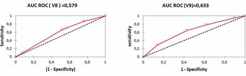
The choice to retain the variable $V_9$ is based on the curve of $ROC$. Indeed, the $AUC$ of the variable $V_9$ is superior to that of the variable $V_8$ . The results of the performance analysis of the two variables are as follows:

Figure 1. Comparison of the performance of correlated variables $V_8$ and $V_9$.

4.2.3. Multivariate analysis and determination of the classification function

Let be $X_j,1\le j\le 12$the quantitative discriminating variables and $T_i,1\le i\le 6$ the qualitative discriminating variables with:

• $(T_i,1\le i\le 6)=\left(q_1,q_6,q_8,q_{12},q_{17},q_{19}\right)$.

• ($X_j,1\le j\le 12)$=($V_1{V}_2,V_3,V_5,V_7,V_9,V_{10},V_{12},V_{13},V_{14},V_{15},V_{16})$.

The multivariate analysis permits the definition of classification functions $f_0$ and $f_1$ of defaulting enterprises and healthy enterprises, respectively, in the Figure 1.

4.2.3.1. The classification function of defaulting enterprises Y = 0

The classification function of defaulting enterprises is defined by:

$f_0=-56,04+0,36\ast X_1+0,01\ast X_2+0,02\ast X_3+0,04\ast X_4-0,03\ast X_5-0,01\ast X_6+0,01\ast X_7+0,1\ast X_8+0,11\ast X_9+0,02\ast X_{10}+0,06\ast X_{11}+0,06\ast X_{12}+0,05\ast T_1+0,08\ast T_2+0,07\ast T_3+0,16\ast T_4+0,55\ast T_5+0,09\ast T_6$

4.2.3.2. The classification function of healthy enterprises Y=1

The classification function of healthy enterprises is defined by:

$f_1=-66,88+0,35\ast X_1+0,01\ast X_2+0,03\ast X_3+0,05\ast X_4+0,02\ast X_5+0,002\ast X_6+0,02\ast X_7+0,1\ast X_8+0,11\ast X_9+0,03\ast X_{10}+0,06\ast X_{11}+0,06\ast X_{12}+0,05\ast T_1+0,09\ast T_2+0,06\ast T_3+0,18\ast T_4+0,71\ast T_5+0,1\ast T_6$

4.2.4. Testing of the significance

The results of the tests of significance defined in the third section are presented as:

The Box’s M test

The results of the test are presented in the Table 17.

Since the calculated p-value is lower than the significance level $\alpha$=0,05, the null hypothesis $H_0$ must be rejected. This means that the model distinguishes between defaulting and healthy enterprises.

Tests relating to the predictive capacity of the score function (Wilks’ lambda)

The results of the test are presented in the Table 18.

Since the calculated p-value is lower than the significance level $\alpha$=0,05, the null hypothesis $H_0$ must be rejected. This means that the model has an acceptable capacity to predict companies in default.

The Confusion matrix

The confusion matrix is presented in the Table 19.

The capacity of the model to classify the company correctly is in the order of 93,7%. This signifies that the model has an excellent capacity to correctly classify enterprises.

Confirmation of this capacity is done using the Q test presented in the third section. The empirical value of the test statistic is:

$Q_{presse}=\frac{{\left(n-\left(n_c\ast p\right)\right)}^2}{n\left(p-1\right)}=1105,89$

The critical value of the ${\chi }^2$ with 1 degree of freedom is equal to 3,84. Since $Q_{presse}$ is superior to the critical value, the null hypothesis $H_0$ must be rejected. This confirms that the model has an excellent capacity to correctly classify enterprises and that it offers a better classification compared to the hazard classification.

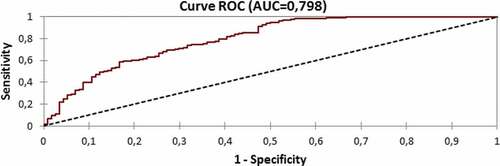
4.2.5. The performance of the model

The $AUC$ of the model is equal to 0,798 which represents an acceptable performance . The results are represented by Figure 2.

Figure 2. Performance of the linear discriminant analysis model.

4.3. The canonical discriminant function

4.3.1. The canonical correlation

The canonical correlation of variables is given by the Table 20.

The canonical correlation of variables is equal to 0,4430. This value does not permit to decide on the discriminating capacity of the model. Indeed, we will support the discriminating capacity of the model on the results of the $AUC$.

4.3.2. The functions at group centroids

The functions at group centroids are presented in the Table 21.

4.3.3. The canonical discriminant function

The number of canonical discriminant functions in the case of two groups is limited to a single function. In our study, this function is presented as follows:

$f_c=-8,031-0,008\ast X_1-0,002\ast X_2+0,003\ast X_3+0,005\ast X_4+0,001\ast X_5+0,003\ast X_6+0,001\ast X_7-0,001\ast X_8+0,001\ast X_9+0,004\ast X_{10}+0,0002\ast X_{11}-0,001\ast X_{12}+0,003\ast T_1+0,004\ast T_2-0,003\ast T_3+0,009\ast T_4+0,086\ast T_5+0,004\ast T_6$

The separation point is equal to zero ($\frac{114\ast \left(-1,6880\right)+1333\ast 0,1440}{1447})$. Indeed, for the prediction of default, a enterprise is considered healthy if $f_c\ge 0$.

The canonical discriminant function shows that the variables most correlated with the score are the return on equity ($X_4$= $\frac{NetProfit}{Equity}$), the seniority of the principal operational staff ($T_4$) and the number of payment incidents in the last 12 months ($T_5$).

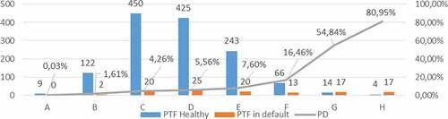
4.4. Conception of the rating model by linear discriminant analysis

The results of the process of the conception of the rating model are presented in the Table 22.

The distribution of healthy and defaulting enterprises and the probability of default by rating class are presented in the Figure 3.

Figure 3. The distribution of healthy and defaulting enterprises and the probability of default by rating class.

4.5. Conception of the notation model using the bayesian approach

For the conception of Bayesian rating models, we opted for an aggregation of the opinions of the selected experts regardless of their weightings. Indeed, the estimation is made with a working group that contains the two categories of experts. Indeed, the results will be weighted at the same time by 25% and 50% to determine the Bayesian models associated with the $LDA$ model.

4.5.1. The explicit probability of default

The results of the assessment of the explicit default probability by rating class are presented as follows:

4.5.2. The implicit probability of default

The implicit probability of default is defined in the Table 23.

$P{D}_{e,K}=\frac{EL}{0,45\ast EAD}$

The results of the assessment of the implicit probability of default by rating class are presented in the Table 24.

The probability of default by experts ($P{D}_{e,K})$ retained is the mean of the explicit and implicit probability of default with a minimum of 0,03% for class A: The Table 25 summarizes the results as follows:

4.5.3. Determination of bayesian rating models

The Bayesian probability of default is a weighting of the experts’ default probability and the default probability determined by the statistical models:

$P{D}_{a,K}=\epsilon \ast P{D}_{e,K}+\left(1-\epsilon \right)\ast P{D}_K$

The Bayesian models according to the weighting of expert opinion are presented in the Table 26.

4.6. Impact of Bayesian modelling on the calculation of unexpected loss (UL)

In Morocco, the legislator has adjusted the formula (4) to take into consideration the characteristics of Moroccan $SMEs$³. Indeed, it provides the following correlation formula for each company (i):

$R_i=0,12\left(\frac{1-e^{-50P{D}_i}}{1-e^{-50}}\right)+0,24\left(1-\frac{1-e^{-50P{D}_i}}{1-e^{-50}}\right)-0,04\left(1-\frac{\left(C{A}_i-10\right)}{165}\right)$

For the $IRB-F$ approach, maturity M for companies is equal to 2,5. As a result, the formula (3) becomes:

$K_i=LG{D}_i\ast \left(N\left(\frac{G\left(P{D}_i\right)+\sqrt{R_i}G\left(0,999\right)}{\sqrt{1-R_i}}\right)-P{D}_i\right)\ast \frac{1}{1-1,5b}$

The weighted assets for each enterprise ($i$) are expressed by:

$RW{A}_i=K_i\ast 12,5\ast EA{D}_i$

The unexpected loss incurred with each company $(i$) is expressed as follows:

$U{L}_i=RW{A}_i\ast 8\mathrm{\%}=K\ast EA{D}_i$

The weighted assets are determined by rating class for each model. Let be $n_{ic},c=A,\dots H$, the size of the class (c), the unexpected loss $U{L}_c$ of class $\left(c\right)$ is defined as follows:

$U{L}_c={\sum }_{i=1}^{n_{ic}}U{L}_i={\sum }_{i=1}^{n_{ic}}RW{A}_i\ast 8\mathrm{\%}$

$\Rightarrow U{L}_c={\sum }_{i=1}^{n_{ic}}{K}_i\ast EA{D}_i$

$\Rightarrow U{L}_c={\sum }_{i=1}^{n_{ic}}LG{D}_i\ast \left(N\left(\frac{G\left(P{D}_i\right)+\sqrt{R_i}G\left(0,999\right)}{\sqrt{1-R_i}}\right)-P{D}_i\right)\ast \frac{1}{1-1,5b}\ast EA{D}_i$

Knowing that the loss given default ($LGD$) in the framework of the $IRB-F$ approach is equal to 45% and that the probability of default ($P{D}_c$) of class (c) is the same for all enterprises in this class, the previous formula is written:

$U{L}_c=0,45\ast \frac{1}{1-1,5b}\ast \left[{\sum }_{i=1}^{n_{ic}}\left(N\left(\frac{G\left(P{D}_c\right)+\sqrt{R_i}G\left(0,999\right)}{\sqrt{1-R_i}}\right)-P{D}_c\right)\ast EA{D}_i\right]$

We pose ${\beta }_c=0,45\ast \frac{1}{1-1,5b}$ thus

$U{L}_c={\beta }_c\ast \left[{\sum }_{i=1}^{n_{ic}}\left(N\left(\frac{G\left(P{D}_c\right)+\sqrt{R_i}G\left(0,999\right)}{\sqrt{1-R_i}}\right)-P{D}_c\right)\ast EA{D}_i\right]$

The total unexpected loss ($UL$) is equal to:

$UL={\sum }_{c=A}^{H}U{L}_c$

4.6.1. The determination of the unexpected loss by LDA

The unexpected loss ($U{L}_0)$ by rating class according to the $LDA$ model is presented in the Table 27.

4.6.2. The Bayesian unexpected loss associated with linear discriminant analysis

The bayesian unexpected loss associated with $LDA$ is presented in the Table 28.

The results show that the Bayesian approach according to the methodology presented above reduces the unexpected loss, respectively, by 4,7% and 10,1%.

5. Conclusion

The measurement of credit risk is a major preoccupation for banks because they have to determine the expected loss to be covered by provisions in the framework of IFRS9 and the unexpected loss that represents the regulatory capital requirement.

The conception of the rating model that classifies counterparties according to their risk profile is the core of the $IRB$ approach. Indeed, several techniques can be used to model the default and determine the different rating classes.

In this paper, we used the linear discriminant analysis to construct a statistical rating model by determining the relationship between the default and the quantitative and qualitative variables of the enterprises.

Then, we proposed a Bayesian approach that permits to integrate the experts’ estimation to calculate the posterior probability of default by rating class. The rating model constructs at the same performance as the statistical model because the adjustment only concerns the probability of default by class.

The proposed approach has several advantages in that it permits the capture of events not taken into account by the statistical model by using the expert opinion such as changes in the economic situation, an increase in the default rate, the various incidents giving rise to the termination of the banking relationship, and changes in the control and decision-making processes.

However, the effectiveness of this approach depends on the rigour of information collection procedures for avoiding an underestimation of default probabilities. Indeed, the Bayesian approach has a major disadvantage related to the quality of information provided by professional experts. As a result, we have presented an approach based on the Delphi technique, proposed the tools for selecting experts and evaluators, and we have determined the steps needed to collect reliable information.

The calculation of the unexpected loss showed that the Bayesian approach reduces the capital requirement. In our empirical study, the lost profit varies between 4,7% and 10,1%.

In summary, the Bayesian approach permits the adjustment of statistical models in order to conform as closely as possible to economic conjuncture and the internal changes in terms of control and decision-making. However, the collection procedures must be very rigorous in order to reduce the risk of the reliability of the information collected from experts.

Additional information

Funding

The authors received no direct funding for this research.

Notes on contributors

Mohamed Habachi

Mohamed Habachi PhD in management science, banking experience of 20 years.

Specialized in Risk Management and Audit.

Two articles published in the field of operational risk and credit risk

Saâd Benbachir

Saâd Benbachir PhD, Studies and Researches in Management Sciences Laboratoy

Director of the Strategic Studies in Law, Economics and Management Center.

31 articles published in market risk, stochastic volatility, operational risk and credit risk.

Notes

1. The correlation formula for companies and banks is $R=0,12\left(\frac{1-e^{-50PD}}{1-e^{-50}}\right)+0,24\left(1-\frac{1-e^{-50PD}}{1-e^{-50}}\right)$. For exposures to SMEs this formula is adjusted to take into account the size of the entity: 0,04 x (1—(S—5)/45)). S is expressed as total annual sales in millions of euros with values of S falling in the range of equal to or less than €50 million or greater than or equal to €5 million. Reported sales of less than €5 million will be treated as if they were equivalent to €5 million. Paragraph 273 of the Basel Committee on Banking Supervision[7].

2. In the case of two groups, Bartlett’s approximation of the lambda distribution is chi-squared with p degrees of freedom $-\left(n-1+\left(p+2\right)/2\right)ln\left(\mathrm{\Lambda }\right)\text{~}{\chi }_p^2$.

3. Bank Al Maghrib’s circular 8/G/2010 considers that SMEs are characterised by a turnover (Sales) that varies between MAD 10 and 175 million $MAD$. The $SMEs$ whose turnover is less than 10 million $MAD$are treated as equivalent to this amount.

Appendix

Table A1. Explanation and significance of quantitative variables

Class	The quantitative variables ($V_j$,$1\le j\le 16$)
$C_1:Activity$	This class determines the impact of the size of the company on the probability of default. Indeed, the size is determined by the turnover, the number of employees, Profit growth and the age of the company;
$V_1$	$V_1$ = Sales or Turnover (ST)
	This variable represents total sales, since a significant turnover is synonymous with the existence of liquidity to honour commitments. As a result, it must be inversely proportional to the probability of default.
$V_2$	$V_2=$ Number of employees
	The size of the company and its stability can be measured by the number of employees
$V_3$	$V_3=$ Profit growth
	Profit growth or decline may be a sign of an upgrading or deterioration of the company’s risk profile
$V_4$	$V_4=$ Age of the company
	The age of the company may explain the failure because new companies are more exposed to failure than older companies. Indeed, in general, the old companies are in a balanced position with regard to the market, to the customers and competitors.
$C_2:Returnofinvestment$	The return on investment is determined by the ratio of net profit to equity and turnover. indeed, low profitability can be synonymous with survival risk and high profitability can be synonymous with a high-risk investment such as high-risk sectors
$V_5$	$V_5=\frac{NetProfit}{Equity}$
	This ratio measures the return on equity. Indeed, low return can mean that the company is having difficulty establishing itself in the market and high return can mean that the company is taking unmeasured risks
$V_6$	$V_6=\frac{NetProfit}{Sales\mathrm{o}\mathrm{r}Turnover\left(ST\right)}$
	This ratio measures the proportion of net profit in turnover. Indeed, a low ratio may mean that the company practices low margins dictated by market conditions or has difficulties mastering the costs of production and marketing. Whereas a high ratio means that sales turnover is high or that the company is dominant in its market so that it can impose these prices by mastering costs.
$C_3:Solvency$	Solvency is measured by the proportion of financial expense in turnover as well as the proportion of debt to equity in the company’s financing. Indeed, high financial costs can be a sign of the company’s difficulty and a high proportion of the debt can mean that the company is over-indebted.
$V_7$	$V_7=\frac{Financialexpenses}{Sales\mathrm{o}\mathrm{r}\mathrm{T}urnover\left(ST\right)}$
	This ratio measures the proportion of financial charges in turnover. a high ratio may mean that the company regularly uses expensive banking services due to long customer lead times payment, lack of liquidity or difficulties in debt collection.
$V_8$	$V_8=\frac{DLMT\left(Debtlongandmeduimterm\right)}{Equity}$
	This ratio measures the proportion of debt log and medium term in the company’s financing. Indeed, a high level of credit financing can mean that the company is over-indebted or small capitalized.
$V_9$	$V_9=\frac{NetDebt}{Equity}$
	Net debt includes $Debtlongandmeduimterm$(DLMT) and short-term debt (DST). As a result, it is an extension of the $V_8$ ratio. in fact, it measures the company’s dependence on debt both in the short term and in the medium and long term
$C_4:Liquidity$	Liquidity represents the ability of current assets to cover current liabilities. Indeed, default depends on the company’s ability to honor these short-term commitments.
$V_{10}$	Let be: A =$\mathrm{A}\mathrm{c}\mathrm{c}\mathrm{o}\mathrm{u}\mathrm{n}\mathrm{t}\mathrm{s}\mathrm{R}\mathrm{e}\mathrm{c}\mathrm{e}\mathrm{i}\mathrm{v}\mathrm{a}\mathrm{b}\mathrm{l}\mathrm{e}$; B =$\mathrm{a}\mathrm{s}\mathrm{s}\mathrm{e}\mathrm{t}\mathrm{s}.\mathrm{C}\mathrm{a}\mathrm{s}\mathrm{h}$; C =$\mathrm{L}\mathrm{i}\mathrm{a}\mathrm{b}\mathrm{i}\mathrm{l}\mathrm{i}\mathrm{t}\mathrm{i}\mathrm{e}\mathrm{s}.\mathrm{C}\mathrm{a}\mathrm{s}\mathrm{h}$; D =$\mathrm{w}\mathrm{o}\mathrm{r}\mathrm{k}\mathrm{i}\mathrm{n}\mathrm{g}\mathrm{c}\mathrm{a}\mathrm{p}\mathrm{i}\mathrm{t}\mathrm{a}\mathrm{l}\mathrm{r}\mathrm{e}\mathrm{q}\mathrm{u}\mathrm{i}\mathrm{r}\mathrm{e}\mathrm{m}\mathrm{e}\mathrm{n}\mathrm{t}\mathrm{s}$; F =$\mathrm{i}\mathrm{n}\mathrm{v}\mathrm{e}\mathrm{n}\mathrm{t}\mathrm{o}\mathrm{r}\mathrm{y}$:
	$V_{10}=\frac{\left(\mathrm{A}+\mathrm{B}\right)}{\left(\mathrm{C}+\mathrm{D}-\mathrm{A}-\mathrm{F}\right)}$
	This ratio represents the rate of coverage of current liabilities and cash liabilities by accounts receivable and cash assets. Indeed, a coverage in excess of 100% is a sign of the company’s solvency.
$C_5:financialstructure$	The financial structure represents the balance between long-term assets and long-term liabilities as well as the proportion of total assets financed by equity.
$V_{11}$	$V_{11}=\frac{WorkingCapital}{CurrentAssets}$
	This ratio represents the proportion of current assets financed by excess of permanent capital over fixed assets. indeed, the company can be in a comfortable position if the coverage rate is significant without going so far as to have an inactive cash position.
$V_{12}$	$V_{12}=\frac{Equity}{TotalAssets}$
	This ratio represents the proportion of equity in the financing of the company’s total assets. Indeed, a low ratio is synonymous with undercapitalization
$C_6:Turnover$	This class is dedicated to the study of the rotation of certain aggregates such as enterprise value, inventory, Accounts receivable and Accounts payable. Indeed, a high rotation is significant for business dynamism and business continuity.
$V_{13}$	$V_{13}=\frac{Sales\mathrm{o}\mathrm{r}\mathrm{T}urnover\left(ST\right)}{Netfixedassets+WCR}$ where WCR is working capital requirement
	The sum of Net fixed assets and WCR of represents the economic value of the company. As a result, this ratio represents the number of times per year that turnover can repay the economic value of the company. Indeed, it means that the company’s activity can repay capital, medium and long-term debts and the working capital requirement a number of times per year equivalent to the value of the ratio.
$V_{14}$	$V_{14}=\frac{inventory}{Sales\mathrm{o}\mathrm{r}Turnover\left(ST\right)}$
	This ratio determines the velocity of stock rotation. Indeed, a high rotation can be synonymous with a dynamic company on its market
$V_{15}$	$V_{15}=\frac{AccountsReceivable}{Sales\mathrm{o}\mathrm{r}Turnove\left(ST\right)}$
	This ratio makes it possible to assess the payment terms granted to customers and the effectiveness of the collection policy. Indeed, a low ratio shows that the company practices short lead times, which can be synonymous with a strong market position and recovery efficiency.
$V_{16}$	$V_{16}=\frac{AccountsPayable}{Totalpurchase}$
	This ratio measures the turnover velocity of supplier credit in relation to total purchases. Indeed, it measures the company’s ability to negotiate payment terms with these suppliers. Supplier credit is measured in number of days of purchases. A high ratio can be synonymous with a solid position of the company with regard to these suppliers.

Appendix

Table A2. Explanation and significance of qualitative variables

Theme	The qualitative variables (${\mathit{q}}_m$,$1\text{lem}\le 19$)
$T_1$: The sector of activity	This theme contains factors external to the company that may correlate with the company’s failure, such as industry, regulation and natural risk.
$q_1$	$q_1=\mathrm{S}\mathrm{e}\mathrm{c}\mathrm{t}\mathrm{o}\mathrm{r}\mathrm{d}\mathrm{e}\mathrm{f}\mathrm{a}\mathrm{u}\mathrm{l}\mathrm{t}\mathrm{r}\mathrm{a}\mathrm{t}\mathrm{e}$
	This variable can explain the company’s default. Indeed, companies in sectors with a high failure rate may have a higher probability of default than companies in sectors with a low failure rate.
$q_2$	$q_2=$ Regulatory impact next year
	Changes in regulations, such as import or export restrictions, increases in taxes, payment delays and labour law, may have a negative impact on the company’s business. consequently, the assessment of the impact of the regulations on the company may influence the default prediction
$q_3$	$q_3=$ Exposure to natural risk
	Climatic conditions can affect the good functioning of certain companies, particularly those in the agri-food sector. As a result, exposure to natural risks such as flooding and drought can have an impact on the probability of default
$T_2$: The company’s positioning and competition	This theme concerns the competitive environment of the company and the difficulties that the company may encounter when setting up. Indeed, the company’s position on the market as well as barriers to entry and national and international competition can have an impact on the company’s failure.
$q_4$	$q_4=\mathrm{C}\mathrm{o}\mathrm{m}\mathrm{p}\mathrm{e}\mathrm{t}\mathrm{i}\mathrm{t}\mathrm{i}\mathrm{v}\mathrm{e}\mathrm{p}\mathrm{o}\mathrm{s}\mathrm{i}\mathrm{t}\mathrm{i}\mathrm{o}\mathrm{n}\mathrm{a}\mathrm{n}\mathrm{d}\mathrm{i}\mathrm{n}\mathrm{t}\mathrm{e}\mathrm{n}\mathrm{s}\mathrm{i}\mathrm{t}\mathrm{y}$
	The company’s position may be monopoly, market leader or among the top 5, top 10 or other. The position may be synonymous with solidity or fragility as a result, it may in some cases explain the default.
$q_5$	$q_5=$ Barriers and new entrants
	The company may be an old or new entrant company and the sector may be open access or requires entry conditions that represent barriers for the company such as technical expertise, a given level of capital, regulatory authorizations etc. The existence or absence of barriers may explain the defaults in certain cases.
$q_6$	$q_6=$ International Competition
	Competition can be national or international. Indeed, for SMEs, international competition can be a major constraint. Consequently, the existence of international competition can encourage default and increase the probability of default.
$T_3$: The concentration and position of the counterparty vis-à-vis its suppliers and customers	The company’s relationship and position with its customers and suppliers can be decisive for its survival and business continuity. Indeed, the company can be a maker or a taker of prices and deadlines with its customers and suppliers, which affects its liquidity. It can also be dependent or independent of its customers and suppliers. As a result, this theme can influence the probability of default.
$q_7$	$q_7=\mathrm{C}\mathrm{u}\mathrm{s}\mathrm{t}\mathrm{o}\mathrm{m}\mathrm{e}\mathrm{r}\mathrm{c}\mathrm{o}\mathrm{n}\mathrm{c}\mathrm{e}\mathrm{n}\mathrm{t}\mathrm{r}\mathrm{a}\mathrm{t}\mathrm{i}\mathrm{o}\mathrm{n}$
	Customer consultation can be crucial for the survival of the company. Indeed, the company may have a single customer, a small number of customers or a diversification of customers. In the first case, the company is dependent on its customer because it can cease its activity following the failure of its customer, the non-conformity of these products and services with the requirements of its customer or following a conflict with him. As a result, the client’s concentration may influence the probability of default.
$q_8$	$q_8=$ Supplier concentration
	The concentration of suppliers can also be decisive for the survival of the company. Indeed, the company may be in a position of strength or weakness vis-à-vis these suppliers because it may suffer if there is only one supplier from the latter’s abuses in terms of price-fixing and payment terms. As a result, supplier concertation can influence the probability of default.
$q_9$	$q_9=$ Positions vis-à-vis suppliers and customers
	The company can be a maker or taker of prices and payment terms with its customers and suppliers, which allows it to define a set of situations defined by the couple (position with regard to the customer, position with regard to the supplier). Each situation can have an impact on the liquidity and cost of products and services. As a result, this variable can influence the probability of default.
$T_4$: Quality and structure of management	This theme integrates all the variables relating to the structure and quality of internal management adopted by the company. Indeed, it covers the capital structure, the experience of the chairmen and senior managers, the successor plan, the timely production of accounting and financial information, historical performance in the event of a crisis and the existence of insurance to cover corporate officers. These variables can influence the probability of default.
$q_{10}$	$q_{10}=\mathrm{S}\mathrm{u}\mathrm{c}\mathrm{c}\mathrm{e}\mathrm{s}\mathrm{s}\mathrm{i}\mathrm{o}\mathrm{n}\mathrm{p}\mathrm{l}\mathrm{a}\mathrm{n}\mathrm{n}\mathrm{i}\mathrm{n}\mathrm{g}\mathrm{a}\mathrm{n}\mathrm{d}\mathrm{b}\mathrm{u}\mathrm{s}\mathrm{i}\mathrm{n}\mathrm{e}\mathrm{s}\mathrm{s}\mathrm{c}\mathrm{o}\mathrm{n}\mathrm{t}\mathrm{i}\mathrm{n}\mathrm{u}\mathrm{i}\mathrm{t}\mathrm{y}$
	The existence of a continuity and succession plan is very important for the survival of the company in the short and long term. Indeed, it ensures that the company is able to ensure the transition in the event of the absence of current managers. The absence of this plan can impact the probability of default.
$q_{11}$	$q_{11}=$ Experience Chairman
	The president’s experience in managing the company, measured in number of years, is an important factor in the company’s survival. Indeed, confirmed experience allows to assure partners about the company’s future, particularly in terms of commercial conflict, debt recovery, banking relations and market mastery. As a result, it can have an impact on the probability of default.
$q_{12}$	$q_{12}=$ Seniority of the principal operational staff
	This variable includes the top managers in the assessment of the probability of default. Indeed, a confirmed experience of the latter can ensure partners on the future of the company, notably in the absence of the president and a succession plan.
$q_{13}$	$q_{13}=\mathrm{C}\mathrm{a}\mathrm{p}\mathrm{i}\mathrm{t}\mathrm{a}\mathrm{l}\mathrm{d}\mathrm{i}\mathrm{s}\mathrm{t}\mathrm{r}\mathrm{i}\mathrm{b}\mathrm{u}\mathrm{t}\mathrm{i}\mathrm{o}\mathrm{n}$
	The concentration of capital in a single hand or in a family represents a high risk because the company will be dependent on the person who has a majority share in the capital. Indeed, a division of capital reduces this risk. As a result, the concentration may increase the probability of default
$q_{14}$	$q_{14}=$ Compliance with the accounting documents delivery schedule
	The timely production of accounting and financial information and its submission to the banker can be synonymous with transparency and better monitoring of the company’s financial situation. The delay can increase partners’ uncertainty about the company’s future, which can lead to an increase in the probability of default.
$q_{15}$	$q_{15}=$ Performance last crisis
	Experience in crisis management is an important indicator of the company’s capacity to surmount difficulties, notably, in terms of liquidity and financing. As a result, this variable permits to adjust the probability of default.
$q_{16}$	$q_{16}=$ Existence of insurance for corporate officers
	Existence of insurance for corporate officers to cover the loss caused by these officers in the event of mismanagement. As a result, it can reduce the probability of default
$T_5$: The company’s history with banking	This theme includes non-payment incidents registered by the bank. Indeed, these incidents are signs of the deterioration of the company’s risk profile. The existence of recent incidents may increase the probability of default.
$q_{17}$	$q_{17}=\mathrm{N}\mathrm{u}\mathrm{m}\mathrm{b}\mathrm{e}\mathrm{r}\mathrm{o}\mathrm{f}\mathrm{p}\mathrm{a}\mathrm{y}\mathrm{m}\mathrm{e}\mathrm{n}\mathrm{t}\mathrm{i}\mathrm{n}\mathrm{c}\mathrm{i}\mathrm{d}\mathrm{e}\mathrm{n}\mathrm{t}\mathrm{s}\mathrm{i}\mathrm{n}\mathrm{t}\mathrm{h}\mathrm{e}\mathrm{l}\mathrm{a}\mathrm{s}\mathrm{t}12\mathrm{m}\mathrm{o}\mathrm{n}\mathrm{t}\mathrm{h}\mathrm{s}$
	This variable represents the number payment incidents. It shows that the company has liquidity problems
$q_{18}$	$q_{18}=\mathrm{P}\mathrm{e}\mathrm{r}\mathrm{c}\mathrm{e}\mathrm{n}\mathrm{t}\mathrm{a}\mathrm{g}\mathrm{e}\mathrm{s}\mathrm{o}\mathrm{f}\mathrm{u}\mathrm{n}\mathrm{p}\mathrm{a}\mathrm{i}\mathrm{d}\mathrm{b}\mathrm{i}\mathrm{l}\mathrm{l}\mathrm{s}\mathrm{o}\mathrm{v}\mathrm{e}\mathrm{r}\mathrm{t}\mathrm{h}\mathrm{e}\mathrm{l}\mathrm{a}\mathrm{s}\mathrm{t}12\mathrm{m}\mathrm{o}\mathrm{n}\mathrm{t}\mathrm{h}\mathrm{s}$
	Similarly, for this variable, it complements the previous one by including commercial paper emitted by the customer and rejected by the bank. It shows that the company has liquidity problems.
$T_6$: $\mathrm{R}\mathrm{e}\mathrm{l}\mathrm{a}\mathrm{t}\mathrm{i}\mathrm{o}\mathrm{n}\mathrm{s}\mathrm{w}\mathrm{i}\mathrm{t}\mathrm{h}\mathrm{b}\mathrm{a}\mathrm{n}\mathrm{k}\mathrm{s}$	This theme concerns the number of banks in relation to the company. Indeed, for small and medium companies, it is preferable for the relationship to be limited to a single bank; this allows the company to benefit from the bank’s advice and to limit the management charge to a single bank. For big companies with a significant financing requirement, it is preferable for banks to form a consortium to finance it in order to prevent the risk of concentration.
$q_{19}$	$q_{19}=\mathrm{N}\mathrm{u}\mathrm{m}\mathrm{b}\mathrm{e}\mathrm{r}\mathrm{o}\mathrm{f}\mathrm{b}\mathrm{a}\mathrm{n}\mathrm{k}\mathrm{s}\mathrm{r}\mathrm{e}\mathrm{l}\mathrm{a}\mathrm{t}\mathrm{e}\mathrm{d}\mathrm{t}\mathrm{o}\mathrm{t}\mathrm{h}\mathrm{e}\mathrm{c}\mathrm{o}\mathrm{m}\mathrm{p}\mathrm{a}\mathrm{n}\mathrm{y}$
	The number of banks in the company must be proportional to its size. The multitude of banks for small and medium-sized structures can be a sign of lack of liquidity and financial mismanagement. As a result, this variable can impact the probability of default

References

- Altman, E. I. (1968, September). Financial ratios, discriminant analysis and the prediction of corporate bankruptcy. Journal of Finance, 23(4), 589–34.
- Ayyub, B. (2001). A practical guide on conducting expert-opinion elicitation of probabilities and consequences for corps facilities. U.S. Army Corps of Engineers Institute.
- Back, B., Laitinen, T., Sere, K., & Wezel, M. V. (1996). Choosing bankruptcy predictors using discriminant analysis, Logit analysis and Genetic Algorithms, Turku Center for computer science. Technical Report, 40, 1–18.
- Bardos, M. (1998). Detecting the risk of company failure at the Banque of France. Journal of Banking and Finance, 22, 1405–1419. doi:10.1016/S0378-4266(98)00062-4
- Basel Committee on Banking Supervision. (1999). Credit risk modelling: Current pratices and applications. Bank for International Settlements.
- Basel Committee on Banking Supervision. (2006). International convergence of capital measurement and capital standards. Bank for International Settlements.
- Basel Committee on Banking Supervision. (2015). Guidance on credit risk and accounting for expected credit losses. Bank for International Settlements.
- Basel Committee on Banking Supervision. (2016). Standardised measurement approach for operational risk, consultative document. Bank For International Settlements.
- Bell, T. B., Ribar, G. S., & Verchio, J. R. (1990), Neural nets vs. logistic regression: A comparison of each model’s ability to predict commercial bank failures. Proceedings of the 1990 Deloitte and Touche-University ofKansas Symposium on Auditing Problems, 29–58.
- Benbachir, S., & Habachi, M. (2018). Assessing the impact of modelling on the Expected Credit Loss (ECL) of a portfolio of small and medium-sized enterprises. Universal Journal of Management, 6(10), 409–431. doi:10.13189/ujm.2018.061005
- Bewick, V., Cheek, L., & Ball, L. (2004). Receiver operating characteristic curves. Critical Care, 8(6), 508–512. doi:10.1186/cc3000
- Bose, I., & Pal, R. (2006). Predicting the survival or failure of click-and-mortar corporations: A knowledge discovery approach. European Journal of Operational Research, 174(2), 959–982. doi:10.1016/j.ejor.2005.05.009
- Bunn, P., & Redwood, V. (2003). Company account based modeling of business failures and the implications for financial stability. The Bank of England’s Working Papers Series N°210.
- Das, S. R., Fan, R., & Geng, G. (2002). Bayesian migration in credit ratings based on probabilities of default. Journal of Fixed Income, 12, 17–23. doi:10.3905/jfi.2002.319329
- Dwyer, D. W. (2006). The Distribution of Defaults and Bayesian Model Validation. Moody KMV.
- Friedman, N., Geiger, D., & Goldszmidt, M. (1997). Bayesian Network Classifiers. Machine Learning, 29(2–3), 131–163. doi:10.1023/A:1007465528199
- Gemela, J. (2001). Financial analysis using bayesian networks. Applied Stochastic Models in Business and Industry, 17(1), 57–67. doi:10.1002/(ISSN)1526-4025
- Giannelloni, J. L., & Vernette, E. (2001). Etudes de marché (pp. 420). édition Vuibert. Paris: Librairie Eyrolles.
- Gôssl, C. (2005). Predictions based on certain uncertainties, A Bayesian credit portfolio approach. Working Paper, Hypo Vereinsbank AG. London.
- Grice, J., & Ingram, R. W. (2001). tests of the generalizability of altman's bankruptcy prediction model. Journal of Business Research, Volume 54 Volume 54 54(Issue 1), 53–61. doi:10.1016/S0148-2963(00)00126-0
- Gurný, P., & Gurný, M. (2013). Comparison of credit scoring models on probability of default estimation for US banks. Prague economic papers. 2, 163-181. doi:10.18267/j.pep.446
- Helmer, O., (1968). “Analysis of the future: The Delphi Method”, https://www.rand.org/content/dam/rand/pubs/papers/2008/P3558.pdf
- Hensher, D. A., Jones, S., William, H., & Greene, W. H. (2007). An error component logit analysis of corporate bankruptcy and insolvency risk in Australia. The Economic Record, 83, 86–103. doi:10.1111/j.1475-4932.2007.00378.x
- Hunter, J., & Isachenkova, N. (2002). A panel analysis of UK industrial company failure. ESRC Centre for Business Research Working Paper 228. Cambridge University.
- Klecka, W. (1980). Discriminant analysis (pp. 16). London: Sage Publications.
- Liang, L., & Wu, D. (2003). An application of pattern recognition on scoring Chinese corporations financial conditions based on back propagation neural network. Computers Et Operations Research, 32, 1115–1120. doi:10.1016/j.cor.2003.09.015
- Ohlson, J. A. (1980). Financial ratios and the probabilistic prediction of bankruptcy. Journal of Accounting Research, 18-1, 109–131. doi:10.2307/2490395
- Oreski, S., Oreski, D., & Oreski, G. (2012). “Hybrid system with genetic algorithm and artificial neural networks and its application to retail credit risk assessment”. Expert Systems with Applications, 39, 12605. doi:10.1016/j.eswa.2012.05.023
- Palm, R. (1999). l’analyse discriminante décisionnelle: principe et applications. Notes stat. Inform. (Gembloux) 99/4, 41p.
- Taffler, R. J. (1982). Forecasting company failure in the UK using discriminant analysis and financial ratio data. Journal of the Royal Statistical Society, Series A, General, 145(3), 342–358. doi:10.2307/2981867
- Tasche, D. (2013). “Bayesian estimation of probabilities of default for low default portfolios”. Journal of Risk Management in Financial Institutions, 6(3), 302–326.
- Zmijeriski, M. (1984). Methodological issues related to the estimation of financial distress prediction models. Journal of Accounting Research, 22, 59–82. doi:10.2307/2490859