The location-inventory model with risk pooling and split demand

Abstract

In the traditional location-inventory system, every demand depot could be served by only one distribution center (DC). This paper relaxes the assumption. The demand depot could be split and served by more than one DC. First, based on the capacitated location-inventory model, the location-inventory model with split demand is presented. Second, the advantage of permitting split and the properties of split are analyzed. Third, in order to solve this new model, a two-phase genetic heuristic algorithm with priority allocating method based on an approximate individual allocating cost are proposed. The results of numerical experiments are compared with non-split version and an important conclusion is illustrated: a small number of split points can make significant cost savings. The results of this study provide a useful reference for location-inventory decision.

Keywords:

• Location-inventory
• genetic heuristic algorithm
• split demand
• safety inventory

PUBLIC INTREST STATEMENT

Location-inventory model could play an important role in integral decision of location and inventory in ecommerce logistics system, which has a great pressure to reduce cost as much as possible. However, in the traditional location-inventory model, the assumption that one demand depot must be served by only one distribution center is not necessary. So, this paper relaxes the assumption and introduces the location-inventory model with split demand. So, its optimal solution is the lower bound of the traditional model since it is the relax of the traditional model. That means the split version has the cost saving advantage compare to the non-split model. In this work, we explore the advantage and the property of the split model. Further, a two-phase genetic heuristic algorithm is developed to solve the new location-inventory model with split demand.

1. Introduction

With the rapid development of e-commerce, the ever-increasing customer demand and operating costs pose significant challenges to the fulfillment operations of e-commerce. In order to improve service level and delivery speed, certain number of distribution centers must be strategically located closely to the associated cities. And the stocks in each distribution center must be set precisely to satisfy the online order. So, both location decisions and inventory decisions play great roles to obtain the competitive advantage of e-commerce. Generally, inventory decisions are greatly affected by the location decisions as the number of DC and the assignment of cities always impact the demand of the DC which is the base of the inventory decisions. Conversely, the location decisions also are affected by the inventory decisions because the transportation cost from DC to its associated cities is affected by the ordering quantities. So, decisions of location and inventory control should be integrated.

For a standard location-inventory problem of e-commerce, the aim is to minimize the average fulfilment cost of integrating location decisions and inventory decisions (Daskin, Coullard, & Shen, 2002; Shen, Coullard, & Daskin, 2003). The location decisions include the optimal number and the location of distribution centers (DCs) and the associated cities should be allocated to DCs. The inventory decisions, help to optimize the inventory level, include the ordering decision and safety stock decisions. In the standard location-inventory problem, each city must be assigned to only one DC. That is, each city is not allowed to be served by more than one DC.

However, in some cases, permit a city be assigned to more than one DC could bring some advantages. A city is assigned to more than one DC means the demand of a city be split to many parts and served by more than one DC. First, splitting of demand may reduce the inventory cost of the logistics network system. The split of demand can get more combination of the demand of cities, to get more opportunity to find some more efficient integrated location-inventory strategy. Second, the split of demand may improve the capacity utilization of DC. When the capacity of DCs is limited, after serve a certain number of associated cities, the left capacity of a DC is not enough to satisfy the whole demand of a city, then the splitting demand could be served by the left capacity. Third, a city could be served by different DCs may reduce the transportation cost because there are more combinations of transportation pairs in the potential possible solutions compare to the none-split version.

The conception of the split demand is originally introduced in the vehicle routing problem (VRP), called VRP with split demand (or the split VRP). In the literature of Dror and Trudeau (1989) and Archetti, Savelsbergh, and Speranza (2006), the advantages of split VRP compare to the non-split VRP has been proved, including the improving of the vehicle utilization and the reducing of the routing cost of VRP solution. Motivated by the idea of split demand in VRP, this paper tends to present the split version of location-inventory problem.

In the split location-inventory problem, the restriction that each city is covered by only one DC is removed. The allocation variables of cities are changed to be real number between 0 and 1 rather than binary. So, we revise the capacitated location-inventory model to the model with split demand. Two simple examples are given to illustrate the advantages of the split. Then, the structural properties of optimal split location-inventory problem solutions are derived. As the split version of location-inventory model is also a non-linear model and is more difficult to solve, a two-phase genetic heuristic algorithm is proposed. At each iteration, the heuristic estimates the individual allocation of each city and decides the split city for each DC as necessary. To show the actual effect of the cost saving of split, we conduct two computational experiments, and compare the results with the non-split version.

To summarize, we list the main contributions of this paper below:

• To begin with, we propose a new model for the location-inventory problem with split demand. The model relax the constraints on city allocation: each city could be allocated to more than one DC as necessary.

• We explore the advantage and the property of the solution in location-inventory problem with split demand. In particular, advantage of the split may be the improvement of capacity utilization of DCs and the combination possibilities of inventory and transportation. The properties could help to decide the possible number of every DC. This allows us to design split location-inventory problem.

• Furthermore, we develop an efficient two-phase heuristic algorithm that allows us to solve the model and builds on its characteristics.

• Last, we show the cost saving of split demand by comparing its results extensively with those of a non-split version location-inventory problem. The split version reaches the highest cost saving of 4.46% in one of the two numerical experiments.

The remainder of this paper is organized as follows. Section 2 reviews the relevant literature. In Section 3, the model of location-inventory with split demand is presented based on the capacitated location-inventory model. Then, two simple examples are proposed to show the advantage of the split. And three key structural properties of the optimal solution are derived in some special conditions. Next, in Section 4, the solution method is analyzed. A two-phase genetic heuristic algorithm with heuristic allocation method is proposed. In Section 5, two computational experiments are presented. Finally, we conclude in Section 6 and give ideas for future work.

2. Related literature

The relevant literature of this study is focus on the location-inventory problems with risk pooling (LIRP) and their solutions. And a brief literature review about the vehicle routing problem with split delivery is reported.

2.1. Location-inventory problem with risk pooling

Risk pooling is a safety stock strategy in the logistics network. Eppen (1979) developed what is known as “risk pooling” in a multi-location newsboy problem with demand consolidated from several facilities. Berman, Krass, and Mahdi Tajbakhsh (2011) verified that the risk pooling can reduce inventory costs by the consolidation of multiple inventory locations into a single location.

Daskin et al. (2002) and Shen et al. (2003) used the idea of risk pooling in order to develop a joint location-inventory problem with unlimited capacity at the warehouses. Their models incorporate fixed facility location cost, working and safety-stock inventory costs at the DCs, transportation costs from the supplier to the DCs, and local delivery costs from the DCs to the retailers.

Ozsen, Coullard, and Daskin (2008) and Miranda and Garrido (2006) developed the capacitated version of the LIRP. Ozsen et al. (2008) only considered the capacity constraints at the warehouses. P A and Garrido (2006) considers two novel capacity constraints. The first constraint states a maximum lot size for the incoming orders to each warehouse, and the second constraint is a stochastic bound regarding inventory capacity.

Recently, the problem has been generalized in different directions. For example, Gebennini, Gamberini, and Manzini (2009) generalizes the model to a dynamic case; Firoozi, Tang, Ariafar, and Ariffin (2013) introduces a quantity discount policy in the model; Silva and Gao (2013) presents the joint replenishment condition; Escalona, Ordóñez, and Marianov (2015) proposes a LIRP with differentiated service levels；Ahmadi-Javid and Hoseinpour (2015) incorporates the price decision into the location-inventory model; Diabat, Abdallah, and Henschel (2015) gives a closed-loop LIRP model. For more detailed review on integrated location-inventory models, we refer the reader to Farahani, Rashidi Bajgan, Fahimnia, and Kaviani (2015). Amiri-Aref, Klibi, and Babai (2018) study the location-inventory model of multi-sourcing. Meissner and Senicheva (2018) and van Wijk and Adan (2019) discuss the transhipment in the location-inventory problem.

All the location-inventory problems in the above literature have a default assumption that each retailer must be served by only one DC. In this article, we relax the assumption and permit each retailer could be split and served by more than one DCs, which could improve the utilization of DC and save the total location and inventory cost.

2.2. Solution methods

Krarup and Pruzan (1983) has proved that the fixed charge location problem (UFLP) is an NP-Hard Problem. Ozsen et al. (2008) think that LIRP model is an extension problem of UFLP by explicitly incorporated inventory decisions into it. Then, we could announce that LIRP is also an NP-Hard Problem, which make it is difficult to solve.

M S et al. (2002) developed a set covering formulation, while Shen et al. (2003) implemented Lagrangian relaxation (LR). Both methods employ the same subproblem, which is solved in O(nlogn) for two special cases: when the variance of the demand is proportional to the mean (as in the Poisson demand case), or when the demand is deterministic. Under this assumption, the objective function could be simplified to be a single nonlinear (concave) form for each retailer, which underlies the efficient solution approach. Based on the same assumption, Ozsen et al. (2008) proposed a Lagrangian method for the capacitated location-inventory problem. Nevertheless, Lagrangian method could not solve the general location-inventory problem without the assumption that the variance of the demand is equal to the mean of demand.

Recently, Atamtürk, Berenguer, and Shen (2012) has given a conic integer programming approach to solve the capacitated location-inventory model, by transform the model to the conic form based on the characters of the binary decision variables. However, the conic integer programming approach is only suitable for the non-split version with the binary allocation variables.

Another stream to solve the NP-hard problem is the heuristic algorithm including the genetic algorithm, Particle Swarm algorithm (De, Wang, & Tiwari, 2019), hybrid algorithm (De, Choudhary, & Tiwari, 2017; 2018), and so on. Silva and Gao (2013) proposes a Greedy Randomized Adaptive Search Procedure (GRASP) to solve the location-inventory problem. Azad and Davoudpour (2008) and Punyim, Karoonsoontawong, Unnikrishnan, and Xie (2018) presents a hybrid Tabu heuristic algorithm to solve capacitated location-inventory problem. Diabat and Deskoores (2016) develops a GA to solve a capacitated location inventory problem. So, based on Diabat and Deskoores (2016), a two-phase heuristic genetic algorithm is presented in this paper.

2.3. Split literature

As mentioned earlier, the research on joint location-inventory problems has almost exclusively assumed the demand depot can only be allocated to one distribution center, they can’t be served by two or more distribution centres. To address the split issue into location-inventory problems, we adopt a split idea in the vehicle routing problem with split deliveries (VRPSD).

The VRPSD is introduced by Dror and Trudeau (1989). They showed how split deliveries could result in savings, both in the total distance traveled and the number of vehicles utilized. Archetti et al. (2006) study the maximum possible savings obtained by allowing split deliveries. Then, VRPSD became a hot issue in the VRP research field and many researchers do the extension study, such as Chen, Golden, and Wasil (2007), Hao and Huili(2015) and Gu, Cattaruzza, and Ogier et al. (2019).

In light of the aforementioned points, one important aim of the current work is to extend the traditional non-split location-inventory problem to account for split permitting. And show how split demand could result in cost savings.

3. Model and split analysis

3.1. Model

Our model is based on the basic capacitated location-inventory model, which was originally studied by Ozsen et al. (2008). Our model assumes the following: for an e-commerce system, certain number of DCs are needed to fulfil the demand of cities in a given certain area. All the cities are the potential location of DCs. Shipments are direct from DCs to cities; Demand at each city is independent and follow Normal distributions. The following notation will be used throughout this paper.

Under the assumptions and the parameters listed above, the joint location-inventory model is formulated as follows:

(1) $Min\sum _{j\in I}\left(f_j{x}_j+\sum _{i\in I}\left(d_{ij}+a_j\right){\mu }_i{y}_{ij}+\left(r_j+g_j\right)\frac{\sum _{i\in I}{\mu }_i{y}_{ij}}{Q_j}+h\frac{Q_j}{2}+z_{\alpha }h\sqrt{L_j\sum _{i\in I}{\sigma }_i^2{y}_{ij}}\right)$(1)

(2) $Q_j+z_{\alpha }\sqrt{L_j\sum _{i\in I}{\sigma }_i^2{y}_{ij}}+L_j\sum _{i\in I}{\mu }_i{y}_{ij}\le C_j,\begin{array}{cc}\hspace{0.17em}& j\in J,\end{array}$(2)

(3) $\sum _{i\in I}{y}_{ij}=1,\begin{array}{cc}\hspace{0.17em}& j\in J,\end{array}$(3)

(4) $y_{ij}\le x_j,\begin{array}{cc}\hspace{0.17em}& i\in I,j\in J\end{array},$(4)

(5) $\begin{array}{cc}\begin{array}{cc}{x}_j\in \left\{0,1\right\},& Q_j\ge 0,\end{array}& j\in J\end{array},$(5)

(6) $\begin{array}{cc}{y}_{ij}\in \left[0,1\right],& i\in I,j\in J\end{array},$(6)

The objective of (1) is to minimize total expected cost of location, shipment, and inventory management. The first objective term is the fixed cost of locating. The second term is the cost of shipping from DC j to the cities and from the supplier plant to DC. The third term in the objective is the expected fixed cost of placing an order at DC and the expected fixed cost per shipment from the central plant to DC. The fourth term is the average inventory holding cost at DC. The fifth term is the expected safety stock cost at DC.

Constraint (2) defines the capacity of each DC to be the sum of the order quantity Qj and the reorder point. Note that in defining the DC capacity, we consider the worst-case scenario, i.e., no demand is observed during lead time. The reorder point is the sum of the safety stock and the expected demand during lead time. Constraint (3) ensures that the demand of each city is satisfied. Constraint (4) guarantee that cities are only assigned to open DCs. Constraints (5) and (6) define the domain of the decision variables.

Compared with the non-split model presented by Ozsen et al. (2008), the similarities and the differences are almost self-explanatory. Clearly, the objective function remains the same. One important difference is the 0–1 allocation variable become a continue variable between 0 and 1.

3.2. Illustration of the advantage of split

As the location-inventory model with split demand is a relax problem of non-split version. So, obviously, the optimal solution of split version model is a lower bound of the optimal solution of non-split version model. So, it is natural that the split version has cost saving advantage compare to the non-split version. In order to get an intuitive illustration about the advantages of split demand in location-inventory problem, two simple examples are shown in this section.

For the capacitated location-inventory model, if the economic ordering quantity (EOQ) of each DC satisfy the capacity limitation, the optimization objective function is similar to the un-capacity version location-inventory model of the Daskin et al. (2002) and Shen et al. (2003). The objective of the model with the working inventory term is given as following:

(7) $Min\sum _{j\in I}\left(f_j{x}_j+\sum _{i\in I}\left(d_{ij}+a_j\right){\mu }_i{y}_{ij}+\sqrt{2h\left(r_j+g_j\right)}\sqrt{\sum _{i\in I}{\mu }_i{y}_{ij}}+z_{\alpha }h\sqrt{L_j\sum _{i\in I}{\sigma }_i^2{y}_{ij}}\right)$(7)

To simplify the problem, the safety inventory, ordering cost and the fixed transportation cost are not considered in the examples. Then, the objective only including three term:

(8) $\sum _{j\in J}{f}_j{x}_j+\sum _{i\in I}{d}_{ij}{\mu }_i{y}_{ij}+\sqrt{2h{r}_j}\sqrt{\sum _{i\in I}{\mu }_i{y}_{ij}}$(8)

Example 1. During a decision horizontal, assume there are three cities with demands u₁ = 3, u₂ = 4, u₃ = 3. All three cities are taken as the potential locations of distribution centers. The unit ordering cost at three points are all equal to 1. The unit transportation cost between the points are: d₁₂ = 1, d₂₃ = 2, d₁₃ = 3; The fix location costs are equal: f₁ = f₃ = f₂ = 6. The unit inventory cost and ordering cost are all equal to 1: h₁ = h₂ = h₃ = 1, r₁ = r₂ = r₃ = 1. The capacities of potential distribution centers in all cities are 5.

Figure 1(a) shows a non-split solution to the location-inventory problem: three distribution centers are set to service its location city. The total cost only includes the fix location cost and the inventory cost, is showed as following.

$3\ast 6+\sqrt{2}\left(\sqrt{4}+\sqrt{3}+\sqrt{3}\right)=25.7274$

Figure 1 (b) shows the split solution to the location-inventory problem: only two distribution centers are set to service three cities, and city 2 is split serviced by both DC 1 and DC 3. The total cost includes the location cost, inventory cost and the transportation cost, is showed as:

$2\ast 6+\sqrt{2}\left(\sqrt{5}+\sqrt{5}\right)+6=24.3426$

Example 1 showed the cost saving of solution of the split demand, which is mainly caused by decreasing the number of DC and inventory cost.

Example 2. Based on the parameter assumption of example 1, only the capacities of potential distribution centers in city 1 and city 2 are changed to be 4 units and 7 units.

Figure 1. (a) The non-split solution and (b) the split solution

The non-split solution is showed in Figure 2 (a). In Figure 2 (a), no split is allowed and the capacity limitation of DC in city 1 is 4. So, city 2 is assigned to the further DC in city 3. The total cost includes the fix location cost, the inventory cost and the transportation cost, is showed as following:

$2\ast 6+\sqrt{2}\left(\sqrt{3}+\sqrt{7}\right)+8=26.1911$

When split allowed, a part of demand of city 2 could be split and served by nearer DC in city 1 (Figure 2 (b)). So, the total cost also includes the location cost, inventory cost and the transportation cost, is showed as:

$2\ast 6+\sqrt{2}\left(\sqrt{6}+\sqrt{4}\right)+5=23.2925$

Example 2 is designed to show the possible transportation cost saving of solution of the split demand.

Figure 2. (a) The non-split solution and (b) the split solution.

3.3. Properties of the optimal solutions of split demand

Motivated by the split VRP, similarly, we presented some properties of the split location-inventory problem under some assumption.

In order to simplify the problem, we also assume the EOQ of each DC can satisfy their capacity limitation, which means the ordering cost and inventory cost terms could simplified like the un-capacitated location-inventory model of Daskin et al. (2002) and Shen et al. (2003). We also assume the variance of the demand of each city to be proportional to the mean demand, in particular, δ_i² = μ_i. Then the objective of the model is simplified as following:

(9) $Min\sum _{j\in I}\left(f_j{x}_j+\sum _{i\in I}\left(d_{ij}+a_j\right){\mu }_i{y}_{ij}+\left(\sqrt{2h\left(r_j+g_j\right)}+z_{\alpha }h\sqrt{L_j}\right)\sqrt{\sum _{i=I}{\mu }_i{y}_{ij}}\right)$(9)

These assumptions make the objective only includes three terms. And the first term is related to the fix location cost, the second term and the third term are related to the mean demand of cities.

Theorem 1: No two distribution center locations in the optimal solution can have more than one split demand point in common.

Proof: For the sake of simplicity, assume two cities p and q with demand d_p, and d_q are served in a split manner by the same two distribution center location 1 and location 2. The quantity (or service) delivered to city p by center 1 is d_1p and by center 2 is d_2p. Similarly define d_1q, and d_2q. (d_1p+ d_2p = d_p; d_1q+d_2q = d_q). This is illustrated in Figure 3. The delivery cost between the demand points and the service depots are c_1p, c_1q, c_2p, c_2q.

Figure 3. The two-distribution center two-split city example.

It is easy to eliminate one of the two-split connects. However, we should prove that the new service structure could decrease the value of the objective function. First, the four deliveries d_1p, d_2p, d_1q, d_2q could be exchanged by three deliveries by the same two distribution center without violating the distribution centers capacity constraints. Let c_min = Min {c_1p+c_2p, c_1q+c_2q}, assume for simplicity that c_min = c_1q+c_2q. Then let d_min = Min {d_1q, d_2q} and assume that d_min = d_1q. Obtain the new quantities delivered to retailer points p and q by routes 1 and 2 as follows:

${d_{1q}}^{\prime }=d_{1q}-d_{1q}=0$, ${d_{2q}}^{\prime }=d_{2q}+d_{1q}$, ${d_{2p}}^{\prime }=d_{2p}-d_{1q}$, ${d_{1p}}^{\prime }=d_{1p}+d_{1q}$

The capacities of the distribution center 1 and 2 are not violated and the total quantities delivered to p and q remain the same as before. One is left with proving that eliminate one connection can results in decreasing (non-increasing) the value of the objective function. As the total demand allocated to the distribution centers are not changed, so the inventory cost doesn’t change. The new total cost function changed only in the transportation cost as follows:

$\mathrm{\Delta }c=d_{1q}\left(c_{1p}+c_{2q}-c_{1q}-c_{2p}\right)$

As we have assumed c_1p + c_2p ≤ c_1q + c_2q, so the cost is decreased.

Next, we present Theorem 2 for which we need the following definition.

Definition: Given k retailer points p₁, p₂, …, p_k and k centers. Center 1 includes the points p₁, p₂; Center 2 includes the points p₂, p₃; center k-1 includes points p_k-1, p_k; And center k includes points p_k, p₁. (This implies that the points p₁, p₂, …, p_k receive split services by the k respective centers and possibly other centers.) We call this subset of demand points, a k-split cycle (show in Figure 4).

Figure 4. k-split cycle of the split deliveries.

Theorem 2: There is no k-split cycle (for any k) in the optimal solution to the SLIRP.

Proof: The proof follows the same argument as in the proof of Theorem 1. Eliminate the least delivery quantity connect of the k-split cycle will decrease the total cost without violating the distribution center capacity constraints.

Theorem 3: The number of splits is less than the number of distribution centers.

Proof: By contradiction. Consider a counterexample to the property with no k-split cycles and the smallest number of the distribution centers. The whole proof process is the same with the property of split-VRP (see in the Archetti et al. (2006)).

4. Solution procedure

4.1. Convex transformation analysis

There are two exist solve method to solve the capacitated location-inventory problem: Lagrangian method (Ozsen et al., 2008) and Conic integer programming approach (Atamtürk et al., 2012). Lagrangian method is a popular solving method of location-inventory problem with a specific assumption that the variance of the demand is equal to the mean of demand, which limit it to be a generate solving method for the split version of location-inventory.

Meanwhile, the Conic integer programming approach is only suitable for the non-split version with the binary allocation variables. In which, the objective of the non-split model is linearized by using t_j and the auxiliary variables for z_j for each city j. Specifically, the following constraint (10) is related with the five term of the objective of formula (1). And constraint (11) is derived from the third term and the fourth term. When no split is allowed, then y_ij is binary and y_ij² = y_ij. Thus, the non-split location-inventory model could be transformed to be a conic convex problem.

(10) $\sum _{i=I}{\sigma }_i{y}_{ij}^2\le t_j^2,\begin{array}{cc}\hspace{0.17em}& \mathrm{\forall }j\in J\end{array}$(10)

(11) $\sum _{i=I}{H}_j{\mu }_i{y}_{ij}^2+{\left(Q_j-\frac{z_j}{2}\right)}^2-\frac{z_j^2}{4}\le 0,\begin{array}{cc}\hspace{0.17em}& \mathrm{\forall }j\in J\end{array}$(11)

However, when the split is permitted, y_ij ∈ [0,1] and y_ij² ≠ y_ij. Then, these two constraints turn back into monomial form and posynomial form as following:

(12) $\sum _{i=I}{\sigma }_i{y}_{ij}\le t_j^2,\begin{array}{cc}\hspace{0.17em}& \mathrm{\forall }j\in J\end{array}$(12)

(13) $\sum _{i=I}{H}_j{\mu }_i{y}_{ij}+{\left(Q_j-\frac{z_j}{2}\right)}^2-\frac{z_j^2}{4}\le 0,\begin{array}{cc}\hspace{0.17em}& \mathrm{\forall }j\in J\end{array}$(13)

Based on conic integer programming model proposed by Atamtürk et al. (2012), the split model can be transformed into a geometric program in log-sum-exp convex form.

(14) $log\left(\sum _{i=I}{e}^{{\hat{y}}_{ij}+2{\hat{t}}_j+b_i}\right)\le 0,\begin{array}{cc}\hspace{0.17em}& \mathrm{\forall }j\in J\end{array}$(14)

(15) $log\left(e^{2{\hat{k}}_j-2{\hat{z}}_j+b^{\ast }}+\sum _{i=I}{e}^{{\hat{y}}_{ij}-2{\hat{z}}_j+{\hat{b}}_{ij}}\right)\le 0,\begin{array}{cc}\hspace{0.17em}& \mathrm{\forall }j\in J\end{array}$(15)

with ${\hat{y}}_{ij}=log{y}_{ij}$, ${\hat{t}}_j=log{t}_j$, $b_i=log{\sigma }_i$, ${\hat{b}}_{ij}=H_j{\mu }_i$, $b^{\ast }=log4$, ${\hat{z}}_j=log{z}_j$, ${\hat{k}}_j=log\left(Q_j-\frac{z_j}{2}\right)$.

However, this convex problem is still very hard to be solved. So, in the next section we proposed a heuristic algorithm to solve the problem.

4.2. Two-phase genetic heuristic method

In this section, we propose a two-phase genetic heuristic method based on approximate individual allocating cost and priority allocating method to solve the new model.

4.2.1. Location search

The evolutionary properties of genetic algorithm can be exploited to determine the location. We represent the chromosome using a binary vector that contains the location decisions including the FDCs alternative locations. Each gene in the chromosome carries a value between 0 and 1, representing for whether a candidate location is selected to locate the FDC (see in Figure 5). Thus, the number of genes in a chromosome is equal to the number of the potential locations.

Figure 5. Individual representation of our GA.

4.2.2. Allocation heuristic method

(1) Individual allocating cost

Once the location of DCs is set, each city should be assigned to an DC. In order to do a quick allocation of the cities, we construct an individual cost function to approximate the real allocating cost.

Based on the objective of un-capacitated location-inventory model (see formulation (7)), only the last three terms, including the transportation cost, the inventory cost and safety stock cost, are strongly related to the assignment of cities. So, we take these three terms as the allocating cost and decomposed them to the individual of every city as their allocating cost when allocating them to DCs. The formulation of approximate allocating cost is:

(16) $c_{ij}={\mu }_i\left(d_{ij}+a_j\right)+\sqrt{2h\left(r_j+g_j\right)}\sqrt{{\mu }_i}+h{z}_{\alpha }\epsilon \sqrt{L_j}{\sigma }_i$(16)

where c_ij is the cost of allocating city i to DC j, ε is an adjustment parameter of safety stock cost. In the allocating cost function (16), the first term is the cost of long-haul transportation and local transportation. The second term is the cost unit of ordering and inventory holding. The third term of function (16) is the safety stock holding cost. The sum of these decomposed individual cost is:

(17) $\sum _{i\in I}{c}_{ik}=\sum _{i\in I}{\mu }_i\left(d_{ij}+a_j\right)+\sqrt{2h\left(r_j+g_j\right)}\sum _{i\in I}\sqrt{{\mu }_i}+h{z}_{\alpha }\sqrt{L_j}\sum _{i\in I}{\sigma }_i$(17)

which is very similar with the last three terms of the objective function (7), which is the approximate of the objective function (1).

In fact, having found the locations of DCs and the allocation of cities, the third decision variable Q_k should be determined according to EOQ and the constrain (2) as follow:

(18) $Q_j^{\ast }=min\left\{EO{Q}_j,Q_j^{limit}\right\}\begin{array}{cc}\hspace{0.17em}& j\in J\end{array}$(18)

where $Q_j^{limit}\le C_k-L_j\sum _{i\in I}{\mu }_i-z_{\alpha }\sqrt{L_j}\sqrt{\sum _{i\in I}{\sigma }_i^2}$

Then, the difference between the cost from objective function (1) and the sum of individual allocation cost (17) is:

(19) $\mathrm{\Delta }=\left[\left(r_j+g_j\right)\frac{\sum _{i\in I}{\mu }_i}{Q_j^{\ast }}+h\frac{Q_j^{\ast }}{2}-\sqrt{2h\left(r_j+g_j\right)}\sum _{i\in I}\sqrt{{\mu }_i}\right]+h{z}_{\alpha }\sqrt{L_j}\left(\epsilon \sum _{i\in I}{\sigma }_i-\sqrt{\sum _{i\in I}{\sigma }_i^2}\right)$(19)

If we set a proper adjustment parameter of safety stock cost, such as:

$\epsilon =\sqrt{\sum _{i\in I}{\sigma }_i^2}/\sum _{i\in I}{\sigma }_i$

Then second term of the cost difference Δ is zero. So, the cost difference Δ only be affected by the first term, which depend on the robust of EOQ.

(2) Priority allocating method

Based on the individual allocating cost, we proposed a way to calculate the priorities of cities to allocate them to DCs. The un-allocated city with the highest priority will be allocated firstly. The priority evaluating formula is:

(20) $p_i=c\left(i,k^{\ast \ast }\left(i\right)\right)-c\left(i,k^{\ast }\left(i\right)\right)$(20)

where p_i is the priority of city i; c(i, k**(i)) is the second lowest allocating cost between city i and DC and c(i, k*(i)) is the lowest allocating cost between city i and DC.

(3) Decide the split cities

According to the given Theorem 3, every chosen distribution center has no more than one split city. So, in our two-phase genetic heuristic method, when the left capacity of DC can’t satisfy the whole demand of the last allocated city, the demand of the last assigned city should be split and the split proportion is:

(21) ${\mathrm{y}}_{\left(i+1\right)j}=C_{left}/\mathrm{\Delta }{Q}_{i+1}$(21)

(22) $C_{left}=C_j-\sqrt{2h\left(r_j+g_j\right)}\sqrt{\sum _{i\in I}{\mu }_i}-z_{\alpha }\sqrt{L_j\sum _{i\in I}{\sigma }_i^2}+L_j\sum _{i\in I}{\mu }_i$(22)

(23) $\mathrm{\Delta }{Q}_{i+1}=\mathrm{\Delta }EOQ+L_j{\mu }_{i+1}+\sqrt{L_j{\sigma }_{i+1}^2}$(23)

However, the optimal ordering quantity of DC with certain assigned cities is difficult to get if the allocation is not finished. To simple the question and get the satisfied solution, we use the EOQ of the DC with cities has allocated to calculate the left capacity of the DC，which is showed as formula (22). Furthermore, as showed in formula (23), we also use EOQ to estimate the change of ordering quantity and take the safety inventory increase as the approximate of the inventory increase when the last city is allocated to the DC. Obviously, the rationality of this heuristic procedure is also dependent on the robust of the EOQ.

4.3. Fitness and other genetic operators

Having found the locations of DCs, the allocation of cities and the split proportion of split point, the third decision variable Q_k should be determined according to EOQ and the equality (18). Then, the objective function for each chromosome can be evaluated. As it is a minimization problem, the fitness function (objective function of the problem) assigns the highest fitness value to the lowest objective function.

Next, the genetic operators, including selection, crossover and mutation should be applied to search for the optimum solution. First, selection method is the roulette selection method, associated a selection probability of each individual chromosome according to its fitness value. Then, the crossover uses randomly created crossover mask to decide the gene get from the parents’ chromosome. Finally, the mutation operator involves generating a random variable for each bit in a sequence. This random variable tells whether a gene will be modified. The parameters of crossover rate and mutation rate of genetic heuristic algorithm could be trial to find the best ones.

5. Computational experiments and results discussion

In this section, two numerical experiments are presented to illustrate this cost saving. One experiment data is extracted from Daskin (1995) since many literatures (Daskin et al. (2002), Shen et al. (2003), Ozsen et al. (2008), Atamtürk et al. (2012)) uses them as the location-inventory benchmark data. We choose the 88-node data from the data set of Daskin (1995) as a typical ecommerce application scene in USA. Similarly, we construct a 31-node data case as a typical ecommerce logistics network in China.

Then, the two-phase genetic heuristic algorithm discussed in the previous sections is used to solve both the split version and the non-split version. We compare the result of split version with the result of the non-split version to show the impact of the split on the solutions. The parameter values of our genetic algorithm are trial to set as following: maximal number of generations is 800, the crossover rate is 0.9, the mutation rate is 0.2.

5.1. Numerical experiments on revised benchmark data

The first numerical experiment in this paper use data from the 1990 U.S. Census described in Daskin (1995). We employ the 88-node data set. However, we need to set the capacities limitation as the original data did not consider the capacity limit. Furthermore, we have noticed that the facility capacities in the data set from Ozsen et al. (2008) were often loose and the facility capacities in the data set from Atamtürk et al. (2012) were too tight. To have DC with a rational capacity limitation, we set the capacities of all the DC are equal to the biggest demand of the cities. So, in 88-node experiment, the capacity is 7400.

To vary the difficulty of problem instances, similar in the literature of Ozsen et al. (2008), β is set as the weight factor associated with the transportation cost. θ is set as the weight factor associated with the inventory cost. Here, we set β and θ values to 0.001 and 0.1 and then to 0.005 and 20.

In Table 2, we report the results obtained by running two-phase genetic heuristic algorithm on both the split version and non-split version of the 88-node data set. We report the objective, the location of the DCs, and the split point for the split version. Focusing on the results obtained by the same solve method, we observe that: first, all the solutions of split version cases have some cost saving compared to the non-split version; second, in the solution of split version, the split happens and the number of split is not more than the number of DCs; the number of DCs do not necessarily decrease the split version compared to the non-split version.

Table 1. The parameters

(µi σ) Demand at each city is independent and follow Normal distributions.

fj: fixed (annual) cost of locating a DC at j, for each j ∈ J;

dij: cost per unit to ship from city j to city i, for each i ∈ I and j ∈ J;

aj: cost per unit of a shipment from the plant to DC j;

rj: fixed administrative and handling cost of placing an order at DC j, for each j ∈ J;

gj: fixed shipment cost per shipment from the plant to DC j;

zα: service level relevant with desired fill rate α;

h: inventory holding cost per unit of product per year;

Lj: lead time of DC j in days;

xj = 1, if retailer j is selected as a distribution center location, and 0 otherwise for each j ∈ J;

yij ∈ [0,1], the proportion of the demand of retailer i is served by a distribution center based at retailer j for each i ∈ I and each j ∈ J.

Table 2. Computational results on the 88-node

β	α	Non-split version		Split version
		Objective	DCs	Objective	DCs	Split points
0.001	0.1	14,088	3-5-7-9-27-30-46-59-67-72	14,013	5-7-18-28-30-33-46-59-67-75	5, 6
0.002	0.1	21,029	3-4-9-15-18-23-28-46-67-72-75-81	20,692	4-5-7-9-15-17-18-28-30-46-47-72	20
0.003	0.1	25,789	3-4-5-7-9-10-15-18-22-26-28-30-32-41-67-72	25,787	3-4-5-7-9-10-15-18-22-26-28-30-32-41-67-72	20
0.004	0.1	29,413	1-2-3-4-5-7-10-12-15-18-22-24-26-28-30-33-36-44-46-51-67	29,343	1-2-3-4-5-7-8-9-10-12-13-15-18-22-23-24-26-30-36-42-46-67	20
0.005	0.1	32,420	1-2-3-4-5-7-8-9-10-12-15-18-23-26-29-30-31-36-38-41-42-44-52	32,391	1-3-4-5-7-8-9-10- 12-13-15-18-22-23-24-26-29-32-34-35-46-47-51-68	20
0.002	0.2	21,284	3-4-5-7-15-28-33-46-47-55-68-72	21,041	3-4-5-7-15-18-30-33-46-67-72	6, 20
0.005	0.5	34,607	1-2-3-4-5-7-8-10-12-13-15-18-22-23-24-30-33-36-41-51-67-76	34,364	1-3-4-5-7-8-9-10-12-13-15-18-22-23-24-26-29-30-32-36-41-42-47	20
0.005	1	36,810	1-2-3-4-5-7-8-9-10-12-13-15-18-22-23-26-29-36-41-47-51-52-68	36,534	1-2-3-4-5-7-8-9-10-12-13-15-18-22–23-24-30-36-41-42-67-76	20
0.005	5	48,600	1-3-4-5-7-9-10-15-18-22-26-28-32-39-51-67-81	48,238	1-2-3-4-5-7-10-15-18-26-28-30-33-41-51-67	20
0.005	10	59,069	1-2-3-4-5-7-9-15-18-30-41-50	59,063	1-2-3-4-5-7-9-15 18-30-41-50	20
0.005	20	77,975	3-4-5-9-15-23-30-32-41-67-72	77,338	1-3-4-5-7-9-15-30 32-46-67	20

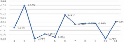
Figure 6 summarizes the cost-reduction percentage of the split version compare with the objective of non-split version. The max reduction percentage is 1.6%.

Figure 6. The percentage cost reduction in the split version of 88-node case.

5.2. Numerical experiments on a new simulation data

To verify the comparison conclusion from the first experiments, the second numerical experiment is necessary. So, we generated a 31-node data based on cities of China using the similar collect method in Daskin (1995). Each of the 31 nodes represents the capital cities and the municipalities. The demand is the total retail sales of consumer goods of the cities. The fixed facility location cost can be obtained by dividing the average house price by 10. The number of the cities are the orders when the cities are ranked in the order of the demands. The capacity is also set as 8400, which is the biggest demand of the cities. Also, in all cases, we set d_ij the unit cost of shipping from candidate DC j to cities i, to the great circle distance between these locations. See Table 1 in Table A1 for the data of 31-node experiment.

In Table 3, we report the results obtained by running two-phase genetic heuristic algorithm on both the split version and non-split version of the 31-node data set. Similarly, we observe the results and find that: all three conclusions found in the first experiment are verified in this second experiment again.

Table 3. Computational results on the 31-node

β	α	Non-split version		Split version
		Objective	DCs	Objective	DCs	Split points
0.001	0.1	30,063	3-4-5-6-7-8-9-10 11-12-13-14-16-19-21-22-25	29,358	3-4-5-7-10-11-12-13-14-16-19-20-21-22-25	5, 9
0.001	0.2	31,254	3-4-5-6-7-8-9-10-11-13-14-15-16-17-19-21-23-25	30,247	3-4-5-7–10-11-13-14-15-16-17-19-20-21-23-25	5, 9, 12
0.001	0.5	32,959	3-4-5-6-7-8-9-10-11-12-13-14-16-19-21-22-25	32,158	3-4-5-7-9-10-11-12-13-14-16-19-20-22-25	5, 9, 21
0.001	1	35,952	3-4-5-6-7-8-9-10-11-13-14-15-16-17-19-21-25	34,688	3-4-5-7-9-10-11-13-14-15-16-17-19-20-25	5, 9, 21, 23
0.001	2	39,968	3-4-5-6-8-9-11-12-16-17-18-25-27	38,367	3-4-5-9-12-16-18-19-20-22-24-25	5, 9, 21, 27, 14
0.001	5	49,658	3-4-6-8-9-11-12-6-17-18-19-22-25	47,794	3-4-5-7-9-12-18-20-22-24-25	5, 9, 28, 14, 15
0.001	10	63,836	3-4-5-6-8-9-16-17-18-24-25-27	60,987	3-4-5-9-12-18-20-22-24-25-27	5, 9, 14, 15, 26

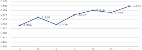
Figure 7 summarizes the cost reduction percentage of the split version in 31-node case. The cost reduction is more obvious than the reduction in first experiment. The max reduction percentage is even higher to be 4.46% in 31-node.

Figure 7. The percentage cost reduction in the split version of 31-node case.

6. Conclusions

This paper studies a location-inventory model with split demand, which is an extension of the traditional capacitated location-inventory model. We relax the constraint that every city must be served by only one DC and permit a city could be served by more than one DCs as necessary. And we assumed that the normal inventory and safety inventory should both served by different DCs according to the assigned split proportion when the demand of the city is split. Then, based on the capacitated location-inventory model, the location-inventory model with split demand is presented. And two simple examples are proposed to show the advantage of the split. Next, inspired by the split VRP, three properties about the structure and the number of the split point of the split location-inventory problem are derived, which could give an approximate way to decide the split points. Furthermore, due to the complexity of the new model, conic integrating programming method can’t be applied any more, we proposed a two-phase genetic heuristic algorithm with an approximate allocation method and approximate split method. Finally, two numerical experiments are presented. The computational results illustrated the advantage of the split and some important conclusions:

1. the great cost-saving effect of the split version compared to the non-split version. The saving percentage can even reach to 4.46%.

2. if splitting is allowed, splitting some points is always a good choice and the number of split points is not more than the number of DCs;

3. the number of DCs do not necessarily decrease in the split version compare to the non-split version.

The main contributions are as follows. First, to our best knowledge, this is the first time to propose location-inventory model with the split demand, which can reduce the total location and inventory cost of the logistics system. Second, the advantage of permitting split demand and the properties are analyzed, which is capable enough to give practical managerial insights for location-inventory by split management. Third, in order to solve this new model, a two-phase genetic heuristic algorithm with priority allocating method based on an approximate individual allocating cost are proposed. The accuracy of this algorithm is mainly based on the robustness of EOQ.

Throughout this paper, there are three analysis are based on EOQ ordering assumption, such as: the analysis of three properties of the split location-inventory model, the calculation of individual allocation cost of city and the estimation of the split proportion of the city, and so on. However, it might be the case that the EOQ formulation sometimes will violate the capacity constraints. Then the decision based on the hypothesis that the order quantities of DCs are EOQs may not be the optimal solution. How will the EOQ assumption affect the objective value of the solution is still unknown. This, in our opinion, provides a promising direction for future research. Another important future direction is to develop more efficient heuristic or hybrid meta-heuristic methods to solve the location-inventory model with split demand, and the heuristic algorithm based on log-sum-exp convex form.

Additional information

Funding

This work was supported by National Natural Science Foundation of China [Grant No. 71461006, No. 71461007 and No. 71761009] and Hainan Province Planning Program of Philosophy and Social Science (HNSK(YB)19-06, HNSK(YB)19-11).

Notes on contributors

Hao Xiong

Hao Xiong is working as a professor and doctoral supervisor in Department of Management Science at Hainan University, China. He had his PhD degree from Tongji University and completed his post-doctoral research at Central South University. He has conducted an academic visitor at Alliance Manchester Business School of the University of Manchester for a year. His areas of research include Operation Research, Tourism management, Inventory control, Vehicle routing problem, E-commerce and Machine learning etc. He has directed many research projects, such as projects from National Natural Science Foundation of China and the project of China Postdoctoral Science Foundation etc. And he has published more than 40 papers in Chinese authoritative journals.

Appendix

Table A1. The second experiment data

City	No.	Latitude	Longitude	Retail sales (ten thousand yuan)	House price (yuan/square meter)
Beijing	1	39.91	116.40	8375.12	4540.00
Shanghai	2	31.24	121.47	8052.00	4186.50
Guangzhou	3	23.13	113.34	6882.85	2096.30
Chongqing	4	29.55	106.55	4599.77	694.20
Tianjin	5	39.10	117.25	4470.43	1800.70
Wuhan	6	30.56	114.38	3916.60	1148.80
Chendu	7	30.71	104.09	3752.88	812.80
Nanjing	8	32.06	118.80	3531.73	2132.00
Hangzhou	9	30.27	120.17	3531.17	1908.90
Shenyang	10	41.83	123.42	3186.09	721.60
Changsha	11	28.21	113.01	2801.97	663.70
Jinan	12	36.65	117.00	2743.35	1107.40
Harbin	13	45.97	126.72	2728.29	742.40
Fuzhou	14	26.08	119.31	2681.72	1564.60
Zhengzhou	15	34.78	113.66	2586.42	1018.80
Xian	16	34.26	108.94	2548.02	695.20
Shijiazhuang	17	38.07	114.49	1972.35	935.50
Changchun	18	43.89	125.32	1970.04	646.70
Kunming	19	25.01	102.70	1702.30	830.40
Hefei	20	31.80	117.26	1480.84	1185.40
Nanning	21	22.65	108.31	1450.84	725.50
Taiyuan	22	37.84	112.52	1281.46	807.20
Huhehaote	23	40.87	111.81	1142.36	653.30
Nanchang	24	28.75	115.83	1132.77	909.20
Wulumuqi	25	43.81	87.61	970.05	662.70
Lanzhou	26	36.08	103.76	843.87	877.00
Guiyang	27	26.54	106.76	785.66	630.40
Haikou	28	20.02	110.33	490.05	766.10
Yinchuan	29	38.48	106.27	348.06	501.70
Xining	30	36.63	101.78	317.46	579.40
Lhasa	31	29.66	91.13	144.11	780.80

References

- Ahmadi-Javid, A., & Hoseinpour, P. (2015). Incorporating location, inventory and price decisions into a supply chain distribution network design problem[J]. Computers & Operations Research, 56, 110–18. doi:10.1016/j.cor.2014.07.014
- Amiri-Aref, M., Klibi, W., & Babai, M. Z. (2018). The multi-sourcing location inventory problem with stochastic demand[J]. European Journal of Operational Research, 266(1), 72–87. doi:10.1016/j.ejor.2017.09.003
- Archetti, C., Savelsbergh, M W., & Speranza, M. G. (2006). Worst-case analysis for split delivery vehicle routing problems[J]. Transportation Science, 40(2), 226–234. doi:10.1287/trsc.1050.0117
- Atamtürk, A., Berenguer, G., & Shen, Z. (2012). A conic integer programming approach to stochastic joint location-inventory problems[J]. Operations Research, 60(2), 366–381. doi:10.1287/opre.1110.1037
- Azad, N., & Davoudpour, H. (2008). A hybrid Tabu-SA algorithm for location-inventory model with considering capacity levels and uncertain demands[J]. Journal of Information and Computing Science, 3(4), 290–304.
- Berman, O., Krass, D., & Mahdi Tajbakhsh, M. (2011). On the benefits of risk pooling in inventory management[J]. Production and Operations Management, 20(1), 57–71. doi:10.1111/poms.2010.20.issue-1
- Chen, S., Golden, B., & Wasil, E. (2007). The split delivery vehicle routing problem: Applications, algorithms, test problems, and computational results[J]. Networks: An International Journal, 49(4), 318–329. doi:10.1002/(ISSN)1097-0037
- Daskin, M S, Coullard, C R, & Shen, Z. M. (2002). An inventory-location model: Formulation, solution algorithm and computational results[J]. Annals of Operations Research, 110(1–4), 83–106. doi:10.1023/A:1020763400324
- Daskin, M.S. (1995). Network and discrete location: Models, algorithms, and applications. New York: Wiley Interscience.
- De, A., Choudhary, A., & Tiwari, M. K. (2017). Multiobjective approach for sustainable ship routing and scheduling with draft restrictions[J]. IEEE Transactions on Engineering Management, 66(1), 35–51. doi:10.1109/TEM.2017.2766443
- De, A., Pratap, S., Kumar, A., & Tiwari, M. K, et al. (2018). A hybrid dynamic berth allocation planning problem with fuel costs considerations for container terminal port using chemical reaction optimization approach[J]. Annals of Operations Research, 1–29. https://doi.org/10.1007/s10479-018-3070-1
- De, A., Wang, J., & Tiwari, M. K. (2019). Hybridizing basic variable neighborhood search with particle swarm optimization for solving sustainable ship routing and bunker management problem[J]. IEEE Transactions on Intelligent Transportation Systems, 1–12. doi:10.1109/TITS.6979
- Diabat, A., Abdallah, T., & Henschel, A. (2015). A closed-loop location-inventory problem with spare parts consideration[J]. Computers & Operations Research, 54, 245–256. doi:10.1016/j.cor.2013.08.023
- Diabat, A., & Deskoores, R. (2016). A hybrid genetic algorithm based heuristic for an integrated supply chain problem[J]. Journal of Manufacturing Systems, 38, 172–180. doi:10.1016/j.jmsy.2015.04.011
- Dror, M., & Trudeau, P. (1989). Savings by split delivery routing[J]. Transportation Science, 23(2), 141–145. doi:10.1287/trsc.23.2.141
- Eppen, G. D. (1979). Note—Effects of centralization on expected costs in a multi-location newsboy problem[J]. Management Science, 25(5), 498–501. doi:10.1287/mnsc.25.5.498
- Escalona, P., Ordóñez, F., & Marianov, V. (2015). Joint location-inventory problem with differentiated service levels using critical level policy[J]. Transportation Research Part E: Logistics and Transportation Review, 83, 141–157. doi:10.1016/j.tre.2015.09.009
- Farahani, R Z, Rashidi Bajgan, H., Fahimnia, B., & Kaviani, M. (2015). Location-inventory problem in supply chains: A modelling review[J]. International Journal of Production Research, 53(12), 3769–3788. doi:10.1080/00207543.2014.988889
- Firoozi, Z., Tang, S H., Ariafar, S., & Ariffin, M. K. A. M. (2013). An optimization approach for a joint location inventory model considering quantity discount policy[J]. Arabian Journal for Science and Engineering, 38(4), 983–991. doi:10.1007/s13369-012-0360-9
- Gebennini, E., Gamberini, R., & Manzini, R. (2009). An integrated production–Distribution model for the dynamic location and allocation problem with safety stock optimization[J]. International Journal of Production Economics, 122(1), 286–304. doi:10.1016/j.ijpe.2009.06.027
- Gu, W., Cattaruzza, D., Ogier, M., & Semet, F., et al. (2019). Adaptive large neighborhood search for the commodity constrained split delivery VRP[J]. Computers & Operations Research, 112:104761. https://doi.org/10.1016/j.cor.2019.07.019
- Hao, X., & HuiLi, Y. (2015). A three-phase tabu search heuristic for the split delivery vehicle routing problem[J]. System Engineering Theory and Practice, 35, 1230–1235.
- Krarup, J., & Pruzan, P. M. (1983). The simple plant location problem: Survey and synthesis[J]. European Journal of Operational Research, 12(1), 36–81. doi:10.1016/0377-2217(83)90181-9
- Meissner, J., & Senicheva, O. V. (2018). Approximate dynamic programming for lateral transshipment problems in multi-location inventory systems[J]. European Journal of Operational Research, 265(1), 49–64. doi:10.1016/j.ejor.2017.06.049
- Miranda, P A, & Garrido, R. A. (2006). A simultaneous inventory control and facility location model with stochastic capacity constraints[J]. Networks and Spatial Economics, 6(1), 39–53. doi:10.1007/s11067-006-7684-5
- Ozsen, L., Coullard, C R., & Daskin, M. S. (2008). Capacitated warehouse location model with risk pooling[J]. Naval Research Logistics (NRL), 55(4), 295–312. doi:10.1002/nav.20282
- Punyim, P., Karoonsoontawong, A., Unnikrishnan, A., & Xie, C. (2018). Tabu search heuristic for joint location-inventory problem with stochastic inventory capacity and practicality constraints[J]. Networks and Spatial Economics, 18(1), 51–84. doi:10.1007/s11067-017-9368-8
- Shen, Z M, Coullard, C., & Daskin, M. S. (2003). A joint location-inventory model[J]. Transportation Science, 37(1), 40–55. doi:10.1287/trsc.37.1.40.12823
- Silva, F., & Gao, L. (2013). A joint replenishment inventory-location model[J]. Networks and Spatial Economics, 13(1), 107–122. doi:10.1007/s11067-012-9174-2
- van Wijk, A., & Adan, I J. (2019). Optimal lateral transshipment policies for a two location inventory problem with multiple demand classes[J]. European Journal of Operational Research, 272(2), 481–495. doi:10.1016/j.ejor.2018.06.033