Multi-objective decision model for green supply chain management

Abstract

In this paper, a multi-objective linear programming model was developed which sought to simultaneously optimize total costs and total GHG emissions for the Thai Rubber supply chain. The model was solved by the ε -constraint method which computed the Pareto optimal solution. Each point in the Pareto set entailed a different design of quantity of rubber product flow between the supply chain entities and transport modes and routes. The result obtained show the trade-offs between costs and GHG emissions. It appears that improvements in cost reductions are only possible by compromising on and allowing for higher GHG emissions. From the Pareto set of solutions, each point is equally effective solution for achieving significant cost reductions without compromising too far on GHG emissions. Scenarios analysis were considered to examine the impact of transportation and distribution restructuring on the trade-off between GHG emissions and costs vis-à-vis the baseline model. Overall, the model developed in this research, together with its Pareto optimal solutions analysis, shows that it can be used as an effective tool to design a new and workable GSCM model for the Thai Rubber industry.

Keywords:

• green supply chain management
• multi-objective optimization
• rubber industry
• GHG emissions

PUBLIC INTEREST STATEMENT

The global rubber industry has witnessed significant growth recently, but efforts to tackle its negative environmental impacts have been limited. This formed the motivation for this study which aims to develop and test a multi-objective decision support model that effectively trades-off environmental performance (GHG emissions) with economic (operational cost) performance. The Thai rubber industry, the world’s largest natural rubber producer is used as the setting. Eight scenarios were considered to examine the impact of transportation and distribution restructuring on the trade-off between GHG emissions and costs vis-à-vis the baseline model. The results show that different GHG emissions target levels will lead to different transport/distribution restructuring strategies for achieving the target. Findings from the study are expected to help policymakers in their supply chain design/redesign decisions so that cost-effective environmental performance improvements can be realized.

1. Introduction

Environmental pollution and global climate change have emerged as one of the major challenges of the twenty-first century with governments worldwide racing to curb their countries’ environmental impacts. This was evident in the recent Paris climate deal where more than 200 countries formally signed an agreement to do this (Salawitch et al., 2017). Thus, industries around the world are looking at options to meet the market demand in a more environmentally responsible way (Dayaratne & Gunawardana, 2015; Habib et al., 2020).

Amongst sectors, rubber-based industries have witnessed significant worldwide growth in recent times (Chanchaichujit & Saavedra-Rosas, 2018; Jawjit et al., 2010) and that is expected to continue in the future; annual growth rate of around 5% is projected for the next 10 years to reach a market size of USD 45 billion globally by 2027 (Kenneth Research, 2019). Today, rubber can be found in more than 50,000 manufactured products today (Rubberworld, 2018). From an environmental standpoint though, the booming rubber industry is a cause for concern given that rubber production is energy-intensive and which also contributes to several environmental pollutions (Dayaratne & Gunawardana, 2015; Jawjit et al., 2015). Importantly, there have been few efforts to tackle its negative environmental impacts (Jawjit et al., 2015).

As in other industries, the environmental consequences of the rubber industry are typically dispersed across different supply chain stages. Greening of the industry, therefore, requires a supply chain-wide focus that includes all key stages and stakeholders; moreover, economic/cost performance implications need to be considered when undertaking environment footprint reduction measures across stages/stakeholders which is essentially the green supply chain management (GSCM) approach/perspective (Rao & Holt, 2005). Given that the rubber industry is struggling to meet the (increased) global demand as also the pressure for cost-competitiveness and environmental friendliness, GSCM is particularly relevant in its case. This forms the motivation for this work which seeks to realize cost-effective improvements in the environmental performance of the rubber industry. The specific objectives are:

1. To develop and apply a multi-objective decision model to achieve trade-offs between environmental and economic performance

2. To conduct multiple scenario analysis for decision support for policymakers

Thailand’s rubber industry was used as the context to test and validate the decision model, and which is because of the following: Thailand is the world’s largest rubber producer (around 5 million tons per year accounting for one-third of the global production (Krungsri Report, 2019); also because the negative environmental impacts from the rubber industry are well recognized there (Pollution Control Department, 2018); and finally because Thailand, is actively engaged in lowering its carbon emissions and developing a climate-resilient society; it not only signed the Kyoto Protocol in 1998 but also developed Nationally Appropriate Mitigation Actions (NAMAs) to lower greenhouse gas emissions below business as usual (BAU) levels by 2020 as well as reduce emissions by a further 20–25% in 2030 compared to the BAU level (ONREPP, 2016). Thailand, therefore, provides an appropriate context for understanding the competing actions required from governments and organizations to lessen the environmental impacts associated with the rubber industry while meeting the increasing global demand of rubber products and sustaining its economic contribution. The latter is equally important given that more than six million people are directly involved in the rubber industry across Thailand (Nobnorb & Fongsuwan, 2015). To date, very few studies on the rubber industry and even fewer on the Thai rubber supply chain have dealt with environmental and economic issues together. The few studies that were conducted (e.g., Chanchaichujit et al., 2016) only attempted a single-objective optimization. Here we have tried to generate a full set of trade-off solutions for both costs and GHG emissions so that (from a set of alternative solutions) the decision-maker can select the most appropriate (from their perspective) supply chain network design.

The rest of the paper is structured as follows: In the next section, the mathematical modeling approaches in GSCM used in previous studies are discussed to identify the appropriate model for this work. In section three, we give an account of the Thai rubber supply chain. Section four describes our model, including the associated data sets, parameters, and decision variables; it also includes mathematical formulations and solution procedures to solve the multi-objective optimization problem. The Pareto optimal solutions to costs and GHG emissions are then presented and discussed in section five. The study concludes in section six by presenting valuable insights obtained from the Pareto optimal solution and its scenarios analysis, with regard to the design of the Thai rubber supply chain model trade-off between environmental and economic performance, limitations and suggestions for future research.

2. Mathematical modelling based approaches in GSCM

The use of optimization models for decision making in GSCM has seen significant interest in recent years (Ansari & Kant, 2017). The optimization modeling is based on mathematical procedures that strive to find the optimum solution under a given set of relevant assumptions, constraints, and data (Coyle et al., 2004). While these models apply several mathematical programming techniques such as linear programming, mixed-integer programming, and non-linear programming (Ansari & Kant, 2017; Srivastava, 2007), the application of single and multi-objective linear programming techniques were found to be the most popular (Ansari & Kant, 2017).

Single objective linear programming models have one objective function requiring optimization. For example, Chanchaichujit et al. (2016) used the single objective linear programming model to find the association between the quantity of rubber product flow between supply chain entities and the transportation mode and route, to minimize total GHG emissions. The authors considered GHG emissions and costs as two single objective functions and found the relationship between GHG emissions and costs to be in conflict with each other. The main limitation of using single objective linear programming models is that policymakers are likely to make decisions that fulfill one objective but jeopardize the other. On the other hand, the advantage of the multi-objective model is that it provides trade-offs between conflicting objectives. Given that GSCM decisions usually involve trade-offs among different incompatible objectives, such a model is, therefore, more reasonable and practical in application terms (Wang et al., 2011). Therefore, it is recommended to consider both environmental and economic criteria as multi-objective functions to capture the trade-offs between the two in the supply chain network subject to defined constraints. (Bloemhof-Ruwaard et al., 2008; Walther et al., 2009) highlighted that achieving a win-win solution between the environment and economic dimensions is difficult in practice and therefore, they suggested seeking effective trade-offs as a way forward for real-world problems.

Previously, the multiple-objective decision-making approach has been extensively used in the field of operational research and related application areas to find non-inferior solutions (Radin, 1998; Rangan & Poolla, 1996). In GSCM, multi-objective optimization has also been considered by different researchers, this involve minimizing total costs or maximizing total profits while simultaneously minimizing environmental impacts (Buddadee et al., 2008; Guillén-Gosálbez et al., 2010; Hugo & Pistikopoulos, 2005; Kim et al., 2010; Wang et al., 2011). In these studies, total costs are generally the summation of supply chain activities costs such as production, inventory, and transportation (You & Wang, 2011) while total profit is expressed in terms of net profit values (Hugo & Pistikopoulos, 2005). For environmental objectives, various measures used include CO2 emissions (Kim et al., 2010; Wang et al., 2011), GHG emissions (You & Wang, 2011), energy consumption (Winebrake et al., 2008) and Global Warming Potential (Buddadee et al., 2008). For example, Sheu (2008) used a linear multi-objective optimization model to optimize the operations of both the nuclear power generation and the corresponding induced-waste reverse logistics. Similarly, (Gabriel et al., 2007) proposed a multi-objective optimization model to simultaneously minimize the biosolids odor as well as processing and distribution costs. Given that the nature of supply chains including their structure, costs, and environmental impacts differ for each sector, separate studies are needed for each including one for rubber given its significant environmental impact. Despite its potential, we did not come across any study that utilized a multiple-objective decision-making approach in GSCM in the rubber industry in any country let alone Thailand. From Thailand’s perspective, we came across only one study (Buddadee et al., 2008) set in the country that applied a multiple-objective decision-making approach in GSCM. This study, on the sugar cane supply chain provides insights on the following: (i) location and size of the ethanol production plants; (ii) the allocation of bagasse from each sugar mill to the corresponding ethanol plant. Global Warming Potential objective is used to represent the impact of all GHG emissions, while economic objectives are captured through the summation of all operational costs.

There are two general approaches to solving multiple-objective problems (Carrillo & Taboada, 2012). The first approach involves the aggregation of all the objective functions into a single composite objective function. Mathematical methods like the weighted sum method, goal programming, or utility functions pertain to this general approach. The output of this method is a single solution. In contrast, multiple objective evolutionary algorithms offer the decision-maker a set of trade-off solutions usually called non dominated solutions or Pareto-optimal solutions (Carrillo & Taboada, 2012). By definition, a Pareto is a set where none of the objective functions can be improved without worsening the value of another objective function (Caramia & Dell’Olmo, 2008). Therefore, the Pareto set of solutions offers a range of alternative solutions; decision-makers can investigate and select the one that most satisfies their preferences (Caramia & Dell’Olmo, 2008).

Among the studies that applied Pareto optimal solutions, You and Wang (2011) applied a multi-objective optimization model to develop a trade-off between total cost and environmental influence in green supply chain network design. The Pareto optimal curve in each scenario showed that the model as an effective tool in strategic planning for green supply chain in terms of the trade-offs between CO₂ emissions and investment costs. Specifically, improving the capacity of the network and increasing the amount of supplies to the facilities decreased CO₂ emissions and total costs for the whole supply chain network. Similarly, You and Wang (2011) used a Pareto optimal solution in their mixed-integer multi-objective decision model to optimize the design of the biomass-to-liquid (BTL) supply chain to simultaneously minimize economic aspects and environmental pollution. The multi-objective model was solved by using the ε -constraint method to produce a Pareto curve representing the trade-offs between optimal costs and environmental performance. Furthermore, a study by (Kim et al., 2010) used a Pareto optimal solution in their multi-objective optimization problem to find trade-offs between freight costs and CO₂ emissions. Their study examined six scenarios for various routes in the East-West European corridor, with different market demands and freight mode capacities. The results showed that the trade-off curves tended to have a linear relationship with freight costs and CO₂ emissions.

3. The Thai rubber supply chain

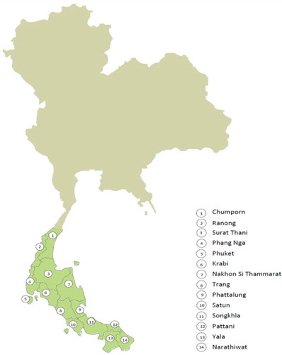
The main rubber plantation and production in Thailand is in Southern part of the country which account for approximately 79% of the total Thai rubber production (Thai Rubber Association [TRA], 2010). It is consisting of 14 provinces in Southern Thailand. These comprise Ranong, Chumporn, Suratthani, Nakhon Si Thammarat, Trang, Phang Nga, Phuket, Krabi, Pattalung, Satun, Songkhla, Pattani, Yala, and Narathiwat. (see Figure 1).

Figure 1. Thai rubber plantation and production

The Thai rubber supply chain is shown in Figure 1 below. As can be seen in the figure, it has divided to rubber plantation, upstream rubber industry and midstream rubber industry. At rubber plantation, farmer grow and harvest rubber to Fresh Latex before delivered to upstream rubber processing plant to processing it into 3 types of upstream rubber products: Field Latex (FL), Unsmoked Sheet (US) and Cup-Lump (CL). Almost all upstream rubber products produced in Thailand will be delivered to midstream rubber industry through trader (dealer, general market, cooperative) before sent to factory processing midstream rubber products of the Concentrated Latex (CL), Block Rubber (BR) and Ripped Smoke Sheet (RS). These products will be delivered to keep as domestic stock or an input for downstream rubber processing such as condom, latex glove, automobile tires, and so on in both domestic and international via 14 routes (R1, R2, R3, R4, R5, R6, R7, R8, R9, R10, R11, R12, R13, R14). R1 to R4 is road freight from midstream rubber processing plants in each province to domestic stock outlet, downstream rubber processing plants, Songkhla port and Penang port for export respectively. R5, R6 and R7 route destination is Penang port. R5 is road freight from midstream rubber processing plants in each province to Padang Basar rail station interchange to rail freight to final destination at Penang port while R6 and R7 is road—rail transportation to Hat Yai rail station and Tung Song rail station respectively before arrived to Padang Basar rail station. R8 is direct road freight to Bangkok port. R9 and R10 is a combination between road and rail to Bangkok port via Hatyai rail station for R9 and Tung song rail station for R10 before arriving to Ladkrabang ICD rail station to continue to Bangkok port. R11 is direct road freight to final destination at Laemchabang port. R12 and R13 is a road and rail transportation to Lamchabang port. R14 is a road and shortsea shipping transportation to Laemchabang port.

Figure 2. Thai rubber supply chain

4. A linear multi-objective optimization model for costs and GHG emissions

A linear programming approach was chosen for studying the association of the quantity of rubber product flow between the supply chain entities at upstream, midstream and downstream rubber industry and the transportation mode and route. The aim was to minimize the total costs and total GHG emissions simultaneously.

There are different techniques for solving problems involving multiple objectives. Guillén-Gosálbez et al. (2010) have classified the techniques for solving multi-objective optimization problems into three approaches. The first approach is based on the transformation of the problem into a single objective and using a single-objective optimization model to solve the problem (Ehrgott, 2005). The second approach is the non-Pareto method which uses search operators based on the objective to be optimized. The general concept of this method can be found in (Blanke et al., 2008). The third approach is the Pareto method. This technique generates a set of solutions to the trade-offs for different objectives (Deb, 2005). This Pareto method will be employed in this study to investigate the trade-offs between cost and GHG emissions minimization in the Thai rubber supply chain. In this way, it will be possible to provide the decision-maker with sufficient alternative options to make trade-off decisions between the objectives (Chanchaichujit et al., 2019).

4.1. Multi-objective optimization and Pareto solutions

In multi-objective optimization problems, no unique solution exists (Deb, 2005). However, there are several solutions that are equal to one another in terms of effectiveness. These solutions are known as Pareto solutions (Miettinen, 2008). The general formulation for multi-objective optimization can be expressed as follows (Blanke et al., 2008):

$Min\left\{f_1\left(x\right),f_2\left(x\right),\dots ,f_k\left(x\right)\right\}$

Subject to $x\in S$

Where

• $k\left(\ge 2\right)$ is the conflicting objective functions $f_i:R^n\to R$, where $R$ denotes the set of real numbers

• The decision variable vectors $x={\left(x_1,x_2,\dots ,x_n\right)}^T$ belong to the non- empty feasible region $S\in R^n$

• Objective vectors are images of decision vectors and consist of the objective function value$z=f\left(x\right)={\left(f_1\left(x\right),f_2\left(x\right),\dots ,f_k\left(x\right)\right)}^T$.

A decision vector $X^{\prime }\in S$is known as Pareto optimal if another $X\in S$does not exist such that $f_i\left(x\right)\le f_i\left(x^{\prime }\right)$ for all $i=1,..,k$ and $f_i\left(x\right)<f_i\left(x^{\prime }\right)$ for at least one index. In multi-objective optimization, objective vectors are regarded as optimal if none of their components can be improved without deterioration to at least one of the other components (Blanke et al., 2008).

4.2. Research methodology and mathematical formulation

This study builds on the work of Chanchaichujit et al. (2016) in which the authors developed a single-objective optimization model for minimizing costs and GHG emissions for the Thai rubber supply chain. The multi-objective optimization model developed in this study includes objective function 1 for cost minimization, objective function 2 for GHG emission minimization and constraints 3–16 for the model constraints (See Tables A1 and B1 in the appendix). The sets, parameters, and decision variables of the multi-objective optimization model used in this study for minimizing costs and GHG emissions optimization are provided in the appendix. These were collected from primary and secondary data sets in the public domain such as the Office of Agricultural Economics (OAE, 2017) and Rubber Authority of Thailand (RRI, 2017). In order to validate the secondary data sets taken from published sources, interviews were conducted for data triangulation. Each Pareto optimal solution within the set represents an alternative to the quantity of rubber product flowing between the supply chain entities and the transportation mode and route, to minimize total costs while at the same time minimizing total GHG emissions. In the next section, the procedure for calculating the Pareto set for the above multi-objective model is explored.

Table B1. Mathematical formulation

Objective function for costs minimization:

$\begin{array}{rl}& Min{Z}_1=\sum _r\sum _f\sum _u\sum _t\sum _g{X}_{rfutg}(C{R}_{fu}+C{T}_{ftg}+C{G}_{gu})+\sum _r\sum _g\sum _p\sum _m\sum _a{Y}_{rgpma}\left(C{T}_{rgp}+C{F}_{pm}+C{T}_{pa}\right)\\ & +\sum _m\sum _a\sum _b\sum _d{Z}_{mabd}\left(C{T}_{ab}+C{M}_b+C{T}_{bd}\right)(1)\end{array}$

Objective function for GHG emissions minimization:

$\begin{array}{rl}& Min{Z}_2=\sum _r\sum _f\sum _u\sum _t\sum _g{X}_{rfutg}(E{R}_{fu}+E{T}_{ftg}+E{G}_{gu})+\sum _r\sum _g\sum _p\sum _m\sum _a{Y}_{rgpma}\\ & \left(E{T}_{rgp}+E{F}_{pm}+E{T}_{pa}\right)+\sum _m\sum _a\sum _b\sum _d{Z}_{mabd}\left(E{T}_{ab}+E{M}_b+E{T}_{bd}\right)(2)\end{array}$

Constraints:

Upstream Rubber Cultivation capacity:

$\sum _u\sum _t\sum _g{X}_{rfutg}\le RP{C}_{fr},\mathrm{\forall }fϵF,\mathrm{\forall }rϵR(3)$

Trader group capacity:

$\sum _f\sum _t{X}_{rfutg}\le TG{C}_{gur},\mathrm{\forall }gϵG,\mathrm{\forall }uϵU,\mathrm{\forall }rϵR(4)$

Midstream rubber processing plant capacity:

$\sum _r\sum _g\sum _a{Y}_{rgpma}\le M{C}_{pm},\mathrm{\forall }pϵP,\text{forallm}ϵM(5)$

Gateway node capacity:

$\sum _r\sum _g\sum _p\sum _m{Y}_{rgpma}\le GW{C}_a,\mathrm{\forall }aϵA(6)$

Freight route system capacity:

$\sum _m\sum _a\sum _d{Z}_{mabd}\le FR{C}_b,\mathrm{\forall }bϵB(7)$

Demand:

$\sum _a\sum _b{Z}_{mabd}=D{E}_{dm},\mathrm{\forall }dϵD,\text{forallm}ϵM(8)$

Production product mix ratio:

$\alpha *\text{left({mathop {}\sum \text{^ }limits\_}r\text{ mathop {}\sum \text{^ }limits\_}g\text{ mathop {}\sum \text{^ }limits\_}p\text{ mathop {}\sum \text{^ }limits\_}a{Y}_{rgpBRa}\text{} right)}+\text{ left({mathop {}\sum \text{^ }limits\_}r\text{ mathop {}\sum \text{^ }limits\_}g\text{ mathop {}\sum \text{^ }limits\_}p\text{ mathop {}\sum \text{^ }limits\_}a{Y}_{rgpRSa}\text{} right)}=\text{mathop {}\sum \text{^ }limits\_}r\text{ mathop {}\sum \text{^ }limits\_}f\text{ mathop {}\sum \text{^ }limits\_}t\text{ mathop {}\sum \text{^ }limits\_}g{X}_{rf\text{US}tg},\forall p\in P,\forall u\in U(9)$

$\left(1-\alpha \right)*\text{left({mathop {}\sum \text{^ }limits\_}r\text{ mathop {}\sum \text{^ }limits\_}g\text{ mathop {}\sum \text{^ }limits\_}p\text{ mathop {}\sum \text{^ }limits\_}a{Y}_{rgpBRa}\text{} right)}=\text{ mathop {}\sum \text{^ }limits\_}r\text{ mathop {}\sum \text{^ }limits\_}f\text{ mathop {}\sum \text{^ }limits\_}t\text{ mathop {}\sum \text{^ }limits\_}g{X}_{rf\text{CL}tg},\forall p\in P,\forall u\in U(10)$

$\text{left({mathop {}\sum \text{^ }limits\_}r\text{ mathop {}\sum \text{^ }limits\_}g\text{ mathop {}\sum \text{^ }limits\_}p\text{ mathop {}\sum \text{^ }limits\_}a{Y}_{rgpCLa}\text{} right)}=\text{ mathop {}\sum \text{^ }limits\_}r\text{ mathop {}\sum \text{^ }limits\_}f\text{ mathop {}\sum \text{^ }limits\_}t\text{ mathop {}\sum \text{^ }limits\_}g{X}_{rfFLtg}(11)$

Conservation flow:

$\sum _r\sum _f\sum _u\sum _t{X}_{rfutg}=\sum _r\sum _p\sum _m\sum _a{Y}_{rgpma},\mathrm{\forall }gϵG(12)$

$\sum _r\sum _g\sum _p{Y}_{rgpma}=\sum _b\sum _d{Z}_{mabd},\text{forallm}ϵM,\mathrm{\forall }aϵA(13)$

Non-negativity constraints:

$X_{rfutg}\ge 0(14)$

$Y_{rgpma}\ge 0(15)$

$Z_{mabd}\ge 0(16)$

4.3. Solution procedure and model implementation

For the calculation of the Pareto set, two basic methods exist in the literature. These are the weighting method and the $\epsilon$ -constraint method (Miettinen, 2008). In recent years, some literature has pointed out the drawbacks of using the weighting method (Arora, 2017; Khan & Rehman, 2013). Arora (2017) highlighted the main weakness of the weighting method as being that, although the weights were chosen consistently and continuously, an even distribution of Pareto optimal points will not necessarily result, thus, there is no guarantee of an accurate representation of the Pareto optimal set. In contrast, previous works in the literature on GSCM have highlighted the advantage of using the $\epsilon$ -constraint method (Caramia & Dell’Olmo, 2008; Gebreslassie et al., 2009; Miettinen, 2008). In addition, the $\epsilon$ -constraint method has been widely used to solve many multi-objective problems in GSCM (for e.g., (Guillén-Gosálbez et al., 2010; Hugo & Pistikopoulos, 2005; Kim et al., 2010). The $\epsilon$-constraint method was therefore used in the study.

In the $\epsilon$-constraint method, one of the objective functions in the original problem was selected for optimization while the other objective was converted into constraints (Caramia & Dell’Olmo, 2008). In this research, $Z_1$ was selected for optimisation and $Z_2$ was formulated as an additional constraint. The right hand value of the additional constraint is $\epsilon$, which represents the limit of GHG emissions. The reformulated model is as follows:

(1) $Min{Z}_1=\sum _r\sum _f\sum _u\sum _t\sum _g{X}_{rfutg}(C{R}_{fu}+C{T}_{ftg}+C{G}_{gu})+\sum _r\sum _g\sum _p\sum _m\sum _a{Y}_{rgpma}\left(C{T}_{rgp}+C{F}_{pm}+C{T}_{pa}\right)+\sum _m\sum _a\sum _b\sum _d{Z}_{mabd}\left(C{T}_{ab}+C{M}_b+C{T}_{bd}\right)$(1)

Subject to:

Constraints 3–16;

$Z_2\le \epsilon$ (additional constraint)

In this model, if the $\epsilon$ parameter is set at $\mathrm{\infty }$ (infinity or a very large number); the resulting model then solves the single-objective problem of total cost minimization. In other words, this formulation is a generalization of the cost minimization model as a single objective. In contrast, if the $\epsilon$ parameter is set to too small, the resulting problem is infeasible. To avoid these two extreme situations, it is first necessary to determine reasonable bounds for the $\epsilon$ parameter.

The procedure to calculate the upper and lower boundaries for the ε parameter with the constraints and estimation of the Pareto solution is as follows:

Step 1: Calculate the lower and upper boundaries for the $\epsilon$ parameter (Denote them as ${\epsilon }_{L}and{\epsilon }_U$ respectively). Based on these boundaries, determine a step ($h$) to be used to define a partition of the interval (${\epsilon }_k={\epsilon }_L+h\cdot k\mathrm{\forall }k\in K$) with $K\subseteq N$ as a finite subset of the natural numbers.

Step 2: For $k\in K$

Step 2.1: Initialize all parameters, objective functions, constraints 3–16, and $\epsilon$.

Step 2.2: Run linear programming single-objective optimization function 1 ($Z_1$) with $\epsilon \mathrm{\_}k$ to obtain the optimal solution for $Z_1$ (denoted by $v_k^{\ast }\left(Z_1\right)$)

Step 2.3: Save the set of ordered values: tuple (${\epsilon }_k,v_k^{\ast }\left(Z_1\right)$)

Step 3: The collection of points $\{({\epsilon }_k,v_k^{\ast }\left(Z_1\right)){\}}_{k\in K}$ is a discrete approximation of the Pareto efficiency frontier.

The intervals between the lower and upper boundaries of $\epsilon$ parameter were partitioned into 50 sub-intervals of equal length. Calculations in the model were then performed to find every possible value for$\epsilon$. The ILOG CPLEX version 12.3 optimization software was used to formulate and solve the model. The respective scope was specified by 10,927 variables subjected to 309 constraints. The multi-objective Pareto solution for the Thai rubber supply chain is presented in the next section.

5. Results and discussions

5.1. Pareto optimal solution

The Pareto set of solutions for minimizing costs and GHG emissions is illustrated in Figure 3 (See Table C1 in the appendix for the corresponding table of the Pareto set of solutions). All the optimal solutions lie on the Pareto curve. Thus, the solutions above the curve are sub-optimal while any solutions below the curve are infeasible. Each point in the Pareto set entails a specific quantity of rubber product flow between the supply chain entities (farmer, trader group and factory) and the transportation modes and routes. The marginal point at the upper left (point A) is the extreme solution for GHG emission minimization whereas the marginal point at the lower right (point C) is the extreme solution for cost minimization.

Figure 3. Pareto curve of costs and GHG emissions

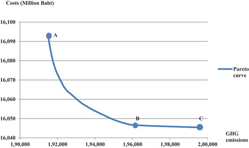
Table C1. The Pareto set of solutions for minimizing costs and GHG emissions using the $\epsilon$ -constraint method

Sub-interval	Parameter value (GHG emissions; Ton)	Costs (Million Baht)
1	199,550	16,045
2	199,390	16,045
3	199,230	16,046
4	199,070	16,046
5	198,910	16,046
6	198,750	16,046
7	198,590	16,046
8	198,430	16,046
9	198,270	16,046
10	198,110	16,046
11	197,950	16,046
12	197,790	16,046
13	197,630	16,046
14	197,470	16,046
15	197,310	16,046
16	197,150	16,046
17	196,990	16,046
18	196,830	16,046
19	196,670	16,046
20	196,510	16,046
21	196,350	16,046
22	196,190	16,047
23	196,030	16,047
24	195,870	16,047
25	195,710	16,047
26	195,550	16,048
27	195,390	16,048
28	195,230	16,049
29	195,070	16,049
30	194,910	16,050
31	194,750	16,050
32	194,590	16,051
33	194,430	16,052
34	194,270	16,053
35	194,110	16,053
36	193,950	16,054
37	193,790	16,055
38	193,630	16,056
39	193,470	16,057
40	193,310	16,058
41	193,150	16,059
42	192,990	16,060
43	192,830	16,062
44	192,670	16,063
45	192,510	16,064
46	192,350	16,066
47	192,190	16,069
48	192,030	16,072
49	191,870	16,076
50	191,710	16,082

The Pareto curve demonstrates the trade-offs between costs and GHG emissions. It shows that GHG emission reduction is only possible by compromising costs (which will be higher). The X and Y-axes in the Pareto graph are GHG emissions in tons and costs in millions of Baht (1 Thai Baht equals 0.033 US dollars). These can be used to indicate changes in costs relative to GHG emissions. As seen in Figure 3, the Pareto curve shows two distinct patterns. The first pattern from point B to point A (right to the left) shows a drastic increase in costs relative to minimal decrements in GHG emissions as the curve moves towards the extreme solution for GHG emission minimization at point A. The second pattern from point C (extreme solution for cost minimization) to point B shows a minimal increase in costs relative to significant decrements in GHG emissions. The Pareto curve is almost a flat line.

From the alternative solutions, policymakers in the Thai rubber industry can choose the best-fit solution, according to preference and applicable policy. Although environmental responsibility is currently voluntary in the industry, policymakers can begin to consider making environmental improvements for a marginal increase in total costs. Although each point in the Pareto curve is equally effective at representing different solutions to or compromises between these two objectives, it is possible to find a “good choice” solution in the above curves. The solution in point B may be a promising answer given that a significant reduction in GHG emissions can be achieved without compromising too much in terms of costs. In addition, the Thai rubber policymakers can use this Pareto curve as a tool to estimate the potential gain in environmental improvements compared with the costs to obtain this gain. The solution in point B shows that to reduce 1 ton of GHG emissions, the compromise must be an increase of 0.01 million Baht in costs.

5.2. Scenario analysis

From the theoretical standpoint, the existing literature agrees that any changes made to transportation and distribution networks are highly likely to influence the costs and environmental impact of the supply chain (Hugo & Pistikopoulos, 2005). Therefore, different likely scenarios are tested to examine the potential impact of transportation restructure and distribution restructure scenarios on the trade-off to assist policymakers in their supply chain redesign decisions.

5.2.1. Transportation restructure scenario analysis- Pareto solutions

Rail freight is widely regarded as an economical and environmentally friendly mode of transport among the four commonly used modes of transportation: road, rail, sea, and air (Kim et al., 2010; Winebrake et al., 2008). Four different scenarios relating to road-rail intermodal transport service capacity were explored when the rail freight service capacity of routes R5, R6, R7, R10, R11, R12, and R13 (see Figure 2 for each route description) was increased by 25% (Scenario 1), 50% (Scenario 2), 75% (Scenario 3) and 100% (Scenario 4) in relation to the baseline model. The descriptions of the transportation scenarios are presented in Table 1.

Table 1. Transportation restructure scenarios

Scenario	Description
1	Increase rail freight service capacity of route R5, R6, R7, R10, R11, R12, R13 by 25%
2	Increase rail freight service capacity of route R5, R6, R7, R10, R11, R12, R13 by 50%
3	Increase rail freight service capacity of route R5, R6, R7,R10, R11, R12, R13 by 75%
4	Increase rail freight service capacity of route R5, R6, R7, R10, R11, R12, R13 by 100%

The Pareto curve for transportation scenarios compared with the baseline model is presented in Figure 4. In the figure, the four scenarios have the same scale in each panel, while the baseline Pareto curve was re-scaled to make comparisons with each of the four scenarios. In each scenario, rail freight capacity is increased by 25% to baseline (See Tables C2–C5 in the appendix for the corresponding table to the Pareto set of solutions for each scenario).

Figure 4. Pareto curves of four transportation scenarios

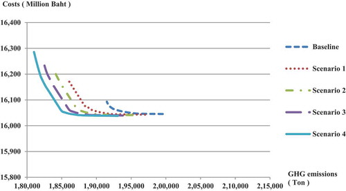
Table C2. The Pareto set of solutions for minimizing costs and GHG emissions using the $\epsilon$ -constraint method: Transportation restructure scenarios 1 (Increase rail freight service capacity by 25% of route R5, R6, R7, R10, R11, R12, R13)

Sub-interval	Parameter value (GHG emissions; Ton)	Costs (Million Baht)
1	197,000	16,043
2	196,772	16,043
3	196,544	16,043
4	196,316	16,043
5	196,088	16,043
6	195,860	16,043
7	195,632	16,043
8	195,404	16,043
9	195,176	16,044
10	194,948	16,044
11	194,720	16,044
12	194,492	16,044
13	194,264	16,044
14	194,036	16,044
15	193,808	16,044
16	193,580	16,044
17	193,352	16,044
18	193,124	16,044
19	192,896	16,044
20	192,668	16,044
21	192,440	16,045
22	192,212	16,045
23	191,984	16,046
24	191,756	16,047
25	191,528	16,047
26	191,300	16,049
27	191,072	16,050
28	190,844	16,051
29	190,616	16,052
30	190,388	16,053
31	190,160	16,054
32	189,932	16,056
33	189,704	16,058
34	189,476	16,060
35	189,248	16,062
36	189,020	16,064
37	188,792	16,071
38	188,564	16,071
39	188,336	16,077
40	188,108	16,085
41	187,880	16,095
42	187,652	16,104
43	187,424	16,114
44	187,196	16,124
45	186,968	16,133
46	186,740	16,143
47	186,512	16,152
48	186,284	16,162
49	186,056	16,172
50	185,828	16,183

Table C3. The Pareto set of solutions for minimizing costs and GHG emissions using the $\epsilon$ -constraint method: Transportation restructure scenarios 2 (Increase rail freight service capacity by 50% of route R5, R6, R7, R10, R11, R12, R13)

Sub-interval	Parameter value (GHG emissions; Ton)	Costs (Million Baht)
1	195,200	16,041
2	194,974	16,041
3	194,748	16,041
4	194,522	16,041
5	194,296	16,041
6	194,070	16,042
7	193,844	16,042
8	193,618	16,042
9	193,392	16,042
10	193,166	16,042
11	192,940	16,042
12	192,714	16,042
13	192,488	16,042
14	192,262	16,042
15	192,036	16,042
16	191,810	16,042
17	191,584	16,042
18	191,358	16,043
19	191,132	16,043
20	190,906	16,043
21	190,680	16,043
22	190,454	16,043
23	190,228	16,044
24	190,002	16,044
25	189,776	16,045
26	189,550	16,046
27	189,324	16,047
28	189,098	16,048
29	188,872	16,050
30	188,646	16,051
31	188,420	16,052
32	188,194	16,054
33	187,968	16,056
34	187,742	16,058
35	187,516	16,060
36	187,290	16,064
37	187,064	16,070
38	186,838	16,079
39	186,612	16,089
40	186,386	16,098
41	186,160	16,108
42	185,934	16,117
43	185,708	16,127
44	185,482	16,136
45	185,256	16,146
46	185,030	16,155
47	184,804	16,166
48	184,578	16,177
49	184,352	16,189
50	184,126	16,201

Table C4. The Pareto set of solutions for minimizing costs and GHG emissions using the $\epsilon$ -constraint method: Transportation restructure scenarios 3 (Increase rail freight service capacity by 75% of route R5, R6, R7, R10, R11, R12, R13)

Sub-interval	Parameter value (GHG emissions; Ton)	Costs (Million Baht)
1	193,800	16,040
2	193,574	16,040
3	193,348	16,040
4	193,122	16,040
5	192,896	16,040
6	192,670	16,040
7	192,444	16,040
8	192,218	16,040
9	191,992	16,040
10	191,766	16,040
11	191,540	16,040
12	191,314	16,040
13	191,088	16,041
14	190,862	16,041
15	190,636	16,041
16	190,410	16,041
17	190,184	16,041
18	189,958	16,041
19	189,732	16,041
20	189,506	16,041
21	189,280	16,041
22	189,054	16,042
23	188,828	16,042
24	188,602	16,043
25	188,376	16,044
26	188,150	16,045
27	187,924	16,046
28	187,698	16,047
29	187,472	16,048
30	187,246	16,049
31	187,020	16,051
32	186,794	16,053
33	186,568	16,055
34	186,342	16,057
35	186,116	16,060
36	185,890	16,068
37	185,664	16,078
38	185,438	16,087
39	185,212	16,096
40	184,986	16,106
41	184,760	16,115
42	184,534	16,125
43	184,308	16,134
44	184,082	16,144
45	183,856	16,153
46	183,630	16,163
47	183,404	16,175
48	183,178	16,186
49	182,952	16,199
50	182,726	16,214

Table C5. The Pareto set of solutions for minimizing costs and GHG emissions using the $\epsilon$ -constraint method: Transportation restructure scenarios 4 (Increase rail freight service capacity by 100% of route R5, R6, R7, R10, R11, R12, R13)

Sub-interval	Parameter value (GHG emissions; Ton)	Costs (Million Baht)
1	193,100	16,038
2	192,858	16,038
3	192,616	16,038
4	192,374	16,038
5	192,132	16,038
6	191,890	16,038
7	191,648	16,039
8	191,406	16,039
9	191,164	16,039
10	190,922	16,039
11	190,680	16,039
12	190,438	16,039
13	190,196	16,039
14	189,954	16,039
15	189,712	16,039
16	189,470	16,039
17	189,228	16,039
18	188,986	16,039
19	188,744	16,040
20	188,502	16,040
21	188,260	16,040
22	188,018	16,040
23	187,776	16,041
24	187,534	16,041
25	187,292	16,042
26	187,050	16,043
27	186,808	16,044
28	186,566	16,045
29	186,324	16,046
30	186,082	16,047
31	185,840	16,048
32	185,598	16,050
33	185,356	16,052
34	185,114	16,054
35	184,872	16,061
36	184,630	16,071
37	184,388	16,081
38	184,146	16,091
39	183,904	16,101
40	183,662	16,111
41	183,420	16,122
42	183,178	16,132
43	182,936	16,142
44	182,694	16,152
45	182,452	16,164
46	182,210	16,177
47	181,968	16,192
48	181,726	16,212
49	181,484	16,235
50	181,242	16,260

These curve patterns strongly suggest that, at the same cost level, an increase in rail freight service capacity leads to lower GHG emissions at the same proportional rate as the increase in rail freight capacity. For the same total GHG emissions, there are two observations related to cost reduction. The first concerns GHG emission levels lower than approximately 190,000 tons. It shows that at the same level of GHG emissions, costs gradually and continuously increase relative to the lower rail freight capacity ratio. The second observation concerns GHG emission levels greater than approximately 190,000 tons. The Pareto curves in all the scenarios become flat and overlapping, meaning that GHG emission levels become increasingly independent of costs. There is no or very minimal increase in costs, but the GHG emissions continue to decrease until entering the realm of extreme solution for GHG emission minimization in which a drastic increase in costs is seen in all scenarios relative to minimal decrements in GHG emissions.

This is a significant finding for policymakers in that any solutions in this curve range may not be effective choices as trade-off solutions. In other words, when GHG emissions reduce to a certain level, it is not worth reducing them further, as a compromise must be made with the greater increases in costs.

It can be seen that when rail freight capacity is increased from the baseline by 25% (Scenario 1), this results in a greater shift of the curve from right to left. The other scenario curves shift (from right to left) consecutively in a relatively smaller proportion. This suggests that an increase in the first 25% of rail freight capacity has a greater influence on the reduction of GHG emissions. Consequently, Scenario 1 may be a more effective solution compared with the other scenarios, particularly when considering that a capacity increase of 25% is a more realistic proposal due to the rail freight capacity expansion limitation (State Railway of Thailand, 2019). However, it is worth observing with regard to Scenarios 2, 3 and 4, that the greater the capacity of the rail freight operation is, the lower the GHG emissions become.

Improvements in rail freight capacity will unavoidably incur investment costs. Therefore, the policymakers must decide whether it is worthwhile to make such improvements, using the Pareto curves as a guide. For example, with GHG emissions reduction as a goal, the policymaker will be able to estimate the cost difference between the baseline and each scenario. If the cost difference is significant enough to cover the investment in rail freight capacity improvement, this goal is worthwhile. Otherwise, the search for alternative trade-off solutions must continue. More specifically, if the Thai rubber industry policymakers set GHG emission levels at 191,500 tons as a goal, the cost difference between the baseline and Scenario 1 is 46 million Baht (costs of 16,093 and 16,047 million Baht for the baseline and Scenario 1, respectively). Thus, if the investment costs of upgrading rail track facilities are lower than 46 million Baht, it is worthwhile pursuing the strategy in Scenario 1.

5.2.2. Distribution restructure scenario analysis—Pareto solutions

This section aims to examine distribution restructure scenario based on (Chanchaichujit et al., 2017)’s work. The author examined the optimum number of gateway nodes for cost and GHG emission minimization in the Thai rubber industry. The results of cost minimization identified an optimum number of four gateway nodes made up of Songkhla, Suratthani, Nakhon Si Thammarat and Trang. For GHG emission minimization results, five provinces were identified as optimum gateway nodes. These were Songkhla, Suratthani, Nakhon Si Thammarat, Trang and Chumporn. The authors also propose the new transportation route R15 for the distribution restructuring in the Thai rubber supply chain. This new route is made up of road-sea intermodal transport. Here, cargo is transported by truck, from its origin to the Kantang coast’s port terminal before being moved by short-sea shipping to Penang (MOT, 2017). Thus, this route is seen as a potential development route for the rubber industry. Figure 5 represents an overview of the optimal network configuration, using the costs and GHG emissions minimization results and new transportation route R15.

Figure 5. Optimum gateway node locations and transportation route R15 (Chanchaichujit et al., 2017)

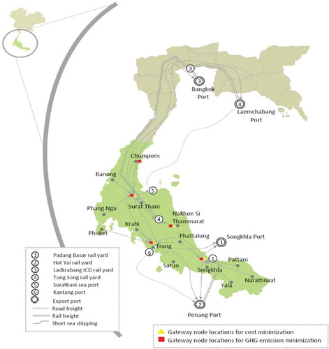
Table 2 shows the distribution restructure scenario analysis considered in this study. This includes the optimal cost solution at four gateway nodes (Scenario 1); optimal cost solution at four gateway nodes with R15 (Scenario 3); optimal GHG emissions at five gateway nodes (Scenario 2); and optimal GHG emissions at five gateway nodes with R15 (Scenario 4). The scenarios with new route R15 aim to provide new insight for policymakers to evaluate the feasibility of developing Kantang port as the western short-sea shipping corridor for the Thai rubber industry.

Table 2. Distribution restructure scenarios

Scenario	Description
1	Four gateway nodes
2	Five gateway nodes
3	Four gateway nodes with new route R15
4	Five gateway nodes with new route R15

Figures 6 and 7 illustrate the Pareto curves for the baseline and four different scenarios related to the distribution restructure (See Tables C6–C9 in the appendix for the corresponding table for the Pareto set of solutions in each scenario). In Figure 6, the Pareto curves only show two visible curves for the baseline and Scenario 4, as the curves for Scenarios 1, 2 and 3 lies under the curve in Scenario 4. Therefore, Figure 7 is presented to view the individual Pareto curves in Scenarios 1, 2 and 3.

Figure 6. Pareto curves of four distribution scenarios (Only baseline and Scenario 4 are visible)

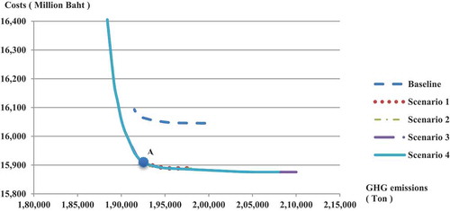
Figure 7. Pareto curves of distribution scenarios 1, 2 and 3

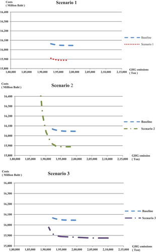
Table C6. The Pareto set of solutions for minimizing costs and GHG emissions using the $\epsilon$ -constraint method: Four distribution node (Trang, Songkhla,Nakhon Si Thammarat, Suratthani)

Sub-interval	Parameter value (GHG emissions; Ton)	Costs (Million Baht)
1	197,500	15,889
2	197,500	15,889
3	197,390	15,889
4	197,280	15,889
5	197,170	15,889
6	197,060	15,889
7	196,950	15,889
8	196,840	15,889
9	196,730	15,889
10	196,620	15,889
11	196,510	15,889
12	196,400	15,889
13	196,290	15,889
14	196,180	15,889
15	196,070	15,889
16	195,960	15,889
17	195,850	15,889
18	195,740	15,889
19	195,630	15,889
20	195,520	15,889
21	195,410	15,889
22	195,300	15,889
23	195,190	15,889
24	195,080	15,890
25	194,970	15,890
26	194,860	15,890
27	194,750	15,890
28	194,640	15,891
29	194,530	15,892
30	194,420	15,892
31	194,310	15,893
32	194,200	15,894
33	194,090	15,894
34	193,980	15,895
35	193,870	15,896
36	193,760	15,897
37	193,650	15,898
38	193,540	15,899
39	193,430	15,900
40	193,320	15,901
41	193,210	15,902
42	193,100	15,903
43	192,990	15,905
44	192,880	15,906
45	192,770	15,908
46	192,660	15,910
47	192,550	15,912
48	192,440	15,914
49	192,330	15,916
50	192,100	15,920

Table C7. The Pareto set of solutions for minimizing costs and GHG emissions using the $\epsilon$ -constraint method: Five distribution node (Trang, Songkhla,Nakhon Si Thammarat, Suratthani, Chumporn)

Sub-interval	Parameter value (GHG emissions; Ton)	Costs (Million Baht)
1	198,000	15,889
2	197,808	15,889
3	197,616	15,889
4	197,424	15,889
5	197,232	15,889
6	197,040	15,889
7	196,848	15,889
8	196,656	15,889
9	196,464	15,889
10	196,272	15,889
11	196,080	15,889
12	195,888	15,889
13	195,696	15,889
14	195,504	15,889
15	195,312	15,889
16	195,120	15,889
17	194,928	15,890
18	194,736	15,890
19	194,544	15,891
20	194,352	15,892
21	194,160	15,893
22	193,968	15,894
23	193,776	15,896
24	193,584	15,896
25	193,392	15,896
26	193,200	15,896
27	193,008	15,903
28	192,816	15,906
29	192,624	15,908
30	192,432	15,912
31	192,240	15,916
32	192,048	15,921
33	191,856	15,928
34	191,664	15,936
35	191,472	15,945
36	191,280	15,958
37	191,088	15,971
38	190,896	15,984
39	190,704	15,997
40	190,512	16,011
41	190,320	16,025
42	190,128	16,039
43	189,936	16,067
44	189,744	16,096
45	189,552	16,126
46	189,360	16,155
47	189,168	16,185
48	188,976	16,223
49	188,784	16,284
50	188,400	16,406

Table C8. The Pareto set of solutions for minimizing costs and GHG emissions using the $\epsilon$ -constraint method: Four distribution node (Trang, Songkhla,Nakhon Si Thammarat, Suratthani) with new transportation route R15

Sub-interval	Parameter value (GHG emissions; Ton)	Costs (Million Baht)
1	210,000	15,876
2	209,620	15,876
3	209,240	15,876
4	208,860	15,876
5	208,480	15,876
6	208,100	15,876
7	207,720	15,876
8	207,340	15,876
9	206,960	15,876
10	206,580	15,876
11	206,200	15,876
12	205,820	15,876
13	205,440	15,876
14	205,060	15,876
15	204,680	15,876
16	204,300	15,876
17	203,920	15,877
18	203,540	15,877
19	203,160	15,877
20	202,780	15,878
21	202,400	15,878
22	202,020	15,879
23	201,640	15,880
24	201,260	15,880
25	200,880	15,881
26	200,500	15,881
27	200,120	15,882
28	199,740	15,882
29	199,360	15,883
30	198,980	15,884
31	198,600	15,884
32	198,220	15,885
33	197,840	15,885
34	197,460	15,886
35	197,080	15,886
36	196,700	15,887
37	196,320	15,887
38	195,940	15,888
39	195,560	15,889
40	195,180	15,889
41	194,800	15,890
42	194,420	15,892
43	194,040	15,894
44	193,660	15,897
45	193,280	15,900
46	192,900	15,904
47	192,520	15,910
48	192,140	15,919
49	191,760	15,932
50	191,000	15,977

Table C9. The Pareto set of solutions for minimizing costs and GHG emissions using the $\epsilon$ -constraint method: Five distribution node (Trang, Songkhla,Nakhon Si Thammarat, Suratthani, Chumporn) with new transportation route R15

Sub-interval	Parameter value (GHG emissions; Ton)	Costs (Million Baht)
1	208,200	15,876
2	207,608	15,876
3	207,216	15,876
4	206,824	15,876
5	206,432	15,876
6	206,040	15,876
7	205,648	15,876
8	205,256	15,876
9	204,864	15,876
10	204,472	15,876
11	204,080	15,876
12	203,688	15,877
13	203,296	15,877
14	202,904	15,878
15	202,512	15,878
16	202,120	15,879
17	201,728	15,879
18	201,336	15,880
19	200,944	15,881
20	200,552	15,881
21	200,160	15,882
22	199,768	15,882
23	199,376	15,883
24	198,984	15,884
25	198,592	15,884
26	198,200	15,885
27	197,808	15,885
28	197,416	15,886
29	197,024	15,886
30	196,632	15,887
31	196,240	15,888
32	195,848	15,888
33	195,456	15,889
34	195,064	15,889
35	194,672	15,891
36	194,280	15,893
37	193,888	15,895
38	193,496	15,898
39	193,104	15,902
40	192,712	15,907
41	192,320	15,914
42	191,928	15,926
43	191,536	15,941
44	191,144	15,967
45	190,752	15,994
46	190,360	16,022
47	189,968	16,062
48	189,576	16,122
49	189,184	16,182
50	188,400	16,406

The Pareto curves for distribution restructure show that at the four gateway nodes, the curve moved sharply to the lower bottom panel (see Figure 7 Scenario 1). Likewise, with the five gateway nodes, the curve moved to the lower bottom of the panel. However, for the five gateway nodes, the curve shape changed with a lengthening of the line to the upper left side (see Figure 7 Scenario 2). The curve pattern suggests that at the same GHG emissions level, the more gateway nodes there are, the lower the cost becomes compared with the baseline scenario. In addition to the curve shape, it can be noted that the Scenario 1 curve is a portion of the Scenario 2 curve.

For Scenarios 3 and 4, when the new transportation route R15 is implemented in conjunction with four and five gateway nodes, the graph shows the same pattern as Scenarios 1 and 2 respectively. In other words, the curve pattern for Scenarios 1 and 3, and Scenarios 2 and 4 are almost the same. The differences between these curves are that the scenario curves for route R15 lengthen in a straight horizontal line to the bottom right panel before entering the zone of the extreme cost minimization solution.

Another important insight from Figures 6 and 7 is that the curves of these four scenarios lie under and overlap each other. The curves clearly show that Scenario 1 is a partial duplication of Scenario 3 while Scenario 2 is a partial duplication of Scenario 4. Overall, scenarios 1, 2 and 3 are part duplications of Scenario 4. In addition, these four curves have the same turning point (point A) on a flat horizontal line. This information suggests that Scenario 4 may be the most promising, with point A as an effective solution to achieving significant GHG emissions reduction without compromising too much on increased costs.

5.3. Comparison of transportation and distribution Pareto solutions

This section aims to present the Pareto curves for the selected transportation and distribution scenarios. As discussed in the previous section, Scenario 1 for transportation is the most realistic scenario for achieving significant GHG emission reductions without compromising too much in terms of increased costs. In addition, Scenario 4, the distribution restructure, is considered to be one of the most promising possibilities for achieving a notable GHG emissions reduction without compromising greatly on increased costs. Therefore, further examining the relationship between these two scenarios’ Pareto optimal curves is worthwhile.

Figure 8 depicts the Pareto curves for transportation in Scenario 1 (see the Scenario 1: T curve), and distribution Scenario 4 (see the Scenario 4: D curve) and the baseline model.

Figure 8. Pareto curves of baseline, Scenario 1 for transportation and Scenario 4 for distribution

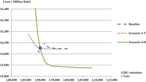
It is clearly illustrated in Figure 8 that at the same cost level, Scenario 1: T indicates lower GHG emissions while at the same GHG emission level, Scenario 4: D exhibits lower costs. The interesting point about this figure is that the Pareto curve of these two scenarios intersects at point A. This is the point where the transportation and distribution scenarios have the same effectiveness. The optimal solution at this point for simultaneous cost and GHG emission reductions would be where GHG measures are taken at a load level of 189,968 tons and the total costs would be 16,062 million Baht. Therefore, if the policymaker were to select this solution, it could be achieved by adopting either Transportation Scenario 1 or Distribution Scenario 4.

For any solution where GHG emission levels are higher than 189,968 tons, Scenario 4: D provides a better compromise. Scenario 4: D indicates a higher cost reduction with a marginal GHG emissions increase than does Scenario 1:T. In contrast, for a GHG emissions level lower than the 189,968 measure, only Scenario 1: T will produce a feasible solution. For this reason, policymakers must focus clearly on GHG emission targets to achieve their goals. It is important to note that different GHG emissions target levels will lead to different strategies for achieving the target by using the best compromise.

In short, the analysis of the Pareto curves in this section shows that the more stringent the GHG emissions target is, the greater the rail operation needed will be. In contrast, if the GHG emissions target is a consideration, but not the ultimate priority, the strategy for achieving environmental gains without increasing costs for trade-offs would be to set up more distribution centers.

6. Implications and conclusion

In this study, a multi-objective linear programming model was developed with the aim of optimizing total costs and total GHG emissions simultaneously for the Thai rubber supply chain. The results obtained in this study show the trade-offs between costs and GHG emissions. It appears that improvements in environmental performance are only possible by compromising on and allowing for higher costs and vice versa. From the Pareto set of solutions, although each point is equally effective in representing a compromise solution, it is possible to identify an effective solution for achieving significant GHG emission reductions without compromising too far on costs.

From the scenario analyses, it can be seen that a transportation restructure is more beneficial to the environment than a distribution restructure is. The greater the increase in rail freight, the lower the GHG emissions in the supply chain. In this study, an increase of 25% in the rail freight capacity was seen as the most feasible scenario leading to lower GHG emissions without significant cost compromises. From an economic perspective, restructuring distribution to five gateway nodes, along with the development of route R15, will result in notable cost reductions.

Overall, this paper showed that the model developed together with its Pareto solutions analysis, can be used as an effective tool to design a new and workable supply chain model that optimizes costs and GHG emissions for the Thai rubber industry.

The study has several practical and research implications. From a practical standpoint, the study provides a decision-support model for the Thai rubber industry policymakers to better manage their supply chain, considering costs and environmental improvements. This includes decisions like whether to facilitate the expansion of or investment in distribution and transportation facilities such as distribution centers, roads, railways and port terminals. The increasing global demand and push for environmental sustainability are putting pressure on Thai rubber industry to increase production levels and remain cost-competitive while minimizing its environmental impacts. Unfortunately, to date, the industry does not have a controlled plan or policy guidelines for the expansion of rubber facilities and transport infrastructure. Therefore, the study is timely in the sense of improving the environmental performance of the Thai rubber industry in an organized manner without losing cost-competitiveness. Moreover, the study is directly aligned with Thailand’s commitment to achieving low GHG emissions, and a climate-resilient society consistent with the strategies of the 12th National Economic and Social Development Plan (NESDP) 2017–2021, and Thailand’s Climate Change Master Plan 2015–2050 (ONREPP, 2016).

In terms of research implications, this research is arguably the first significant attempt to apply a multi-objective decision model to the rubber industry anywhere, let alone in Thailand. Therefore, the contributions of this study are novel. Further researchers could adapt, test and validate this model in other leading rubber-producing countries such as Malaysia, Indonesia, Vietnam and China.

The study has some limitations. It fails to consider the uncertainty inherent in real-world rubber production and distribution networks. Therefore, to address this limitation, future research could consider input uncertainties such as demand, supply, and price. For instance, uncertain rubber production capacities and yield per farm, rubber demand and rubber prices may be incorporated into the model as uncertain parameters. In addition, there could be other potential optimal scenarios that have not been accounted for in this study. The other concern is that the Pareto-optimal solutions sets are typically vast, and the decision-maker usually faces the problem of reducing the size of the set to have a manageable number of solutions to analyze.

Despite the limitations, we think that the application of the proposed model and findings of this study can significantly contribute toward the greening efforts of the rubber industry sector, as well as encourage more research in this field.

Additional information

Funding

The authors received no direct funding for this research.

Notes on contributors

Janya Chanchaichujit

Janya Chanchaichujit is an Assistant Professor in Logistics Management in the School of Management at Walailak University in Thailand. Dr. Chanchaichujit has over twenty years industrial, project consultancy and academic work experience. Her research interest focuses on incorporating various aspects of operational research applications, and technologies into the design and operation of sustainable supply chain management.

Sreejith Balasubramanian

Sreejith Balasubramanian is a Senior Lecturer in Supply Chain Management, and Chair of the Research Committee at Middlesex University, Dubai. His areas of expertise include supply chain, operations management, and sustainability. He is also an expert data analyst with skills in statistical modeling and forecasting.

Vinaya Shukla

Vinaya Shuka is a Senior Lecturer in Operations and Supply Chain Management at Middlesex University Business School, London. Prior to academia, he spent many years as a Management Consultant. His research interests are in green supply chain management, supply chain systems and supply chain risk management.

Appendix A.

Table A1. Model notation

Set
$rϵR$	Set of plantation areas ($r$ = 1,2,3,4,5,6,7,8,9,10,11,12,13,14)
$uϵU$	Set of upstream rubber products ($u$ = Field Latex (FL), Unsmoked Sheet (US), Cup-Lump (CL))
$fϵF$	Set of farmer sizes ($f$ = small, medium, large)
$tϵT$	Set of truck types ($t$ = 4 wheels, 10 wheels) $gϵG$ Set of trader groups ($g$ = dealer, general market, cooperative)
$pϵP$	Set of midstream rubber processing plants ($p$ = summation of all plants in plantation area: 1,2,3,4,5,6,7,8,910,11,12,13,14)
$mϵM$	Set of midstream rubber products ($m$= Concentrated Latex (CL), Ripped Smoked Sheet (RS), Block Rubber (BR))
$aϵA$	Set of gateway nodes ($a$ = 3 (Suratthani), 7 (Nakhon Si Thammarat), 11(Songkhla))
$bϵB$	Set of intermodal freight routes ($b$ = R,R2,R3,R4, … R14)
$dϵD$	Set of domestic destinations and exporting ports ($d$ = Country stock, Midstream Rubber Processing, Songkhla port, Penang port, Bangkok port, Lamchabang port) $\alpha$Mixing parameters
Decision Variables
$X_{rfutg}$	Amount of upstream rubber product $u$ produce from farmer $f$ in plantation area $r$transported by truck type $t$ to trader group $g$
$Y_{rgpma}$	Amount of upstream rubber product$u$ from trader group $g$in plantation area $r$ transported to midstream processing plant $p$ to produce midstream rubber product $m$ and then transported to gateway node $a$ $Z_{mabd}$ Amount of midstream rubber product $m$ from gateway node $a$transported by intermodal freight route $b$ to domestic destinations and exporting port $d$
Data and	Parameters
$RP{C}_{fr}$	Aggregated upstream rubber cultivation capacity of farmer $f$ in each plantation area $r$
$TG{C}_{gur}$	Aggregated trader group capacity of a given trader group $g$ for upstream rubber product u in each plantation area $r$
$M{C}_{pm}$	Aggregated midstream rubber processing plant production capacity of midstream rubber product $m$in a given midstream rubber processing plant $p$
$GW{C}_a$	Aggregated gateway node capacity in a given gateway node $a$
$FR{C}_b$	Aggregated freight route capacity for a given freight route $b$
$D{E}_{dm}$	Aggregated demand for midstream rubber product $m$at destination $d$
Cost	Parameters
$C{R}_{fu}$	Costs of farmer $f$ to process upstream rubber product $u$
$C{T}_{ftg}$	Costs of transport upstream rubber product from farmer $f$ to trader group $g$ by truck type $t$
$C{G}_{gu}$	Costs of trading upstream rubber product $u$ in trader group $g$
$C{T}_{rgp}$	Costs of transport upstream rubber product from trader group $g$ in plantation area $r$ to midstream rubber processing plant $p$
$C{F}_{pm}$	Costs of midstream rubber processing $p$to process midstream rubber product $m$
$C{T}_{pa}$	Costs of transport midstream rubber product from midstream rubber processing plant $p$ to gateway node $a$
$C{T}_{ab}$	Costs of transport midstream rubber product from gateway node $a$ to freight route $b$
$C{M}_b$	Costs of exporting midstream rubber product via freight route $b$
$C{T}_{bd}$	Costs of transport midstream rubber product from freight route $b$ to destination $d$
Environmental Parameters
$E{R}_{fu}$	GHG emissions of farmer $f$ to process upstream rubber product $u$
$E{T}_{ftg}$	GHG emissions of transport upstream rubber product from farmer $f$ to trader group $g$ by truck type $t$
$E{G}_{gu}$	GHG emissions of trading upstream rubber product $u$ in trader group $g$
$E{T}_{rgp}$	GHG emissions of transport upstream rubber product from trader group $g$ in plantation area $r$ to midstream rubber processing plant $p$
$E{F}_{pm}$	GHG emissions of midstream rubber processing $p$to process midstream rubber product $m$
$E{T}_{pa}$	GHG emissions of transport midstream rubber product from midstream rubber processing plant $p$ to gateway node $a$
$E{T}_{ab}$	GHG emissions of transport midstream rubber product from gateway node $a$ to freight route $b$
$E{M}_b$	GHG emissions of exporting midstream rubber product via freight route $b$
$E{T}_{bd}$	GHG emissions of transport midstream rubber product from freight route $b$ to destination $d$

Appendix B.

Appendix C.

References

- Ansari, Z. N., & Kant, R. (2017). Exploring the framework development status for sustainability in supply chain management: A systematic literature synthesis and future research directions. Business Strategy and the Environment, 26(7), 873–33. https://doi.org/10.1002/bse.1945
- Arora, J. S. (2017). Introduction to optimum design (4th ed.). Academic Press.
- Blanke, J., Deb, K., Miettinen, K., & Slowinski, R. (2008). Lecture notes in computer science: Multiobjective optimization, interactive and evolutionary approaches (Vol. 5252). Springer. https://doi.org/10.1007/978-3-540-88908-3
- Bloemhof-Ruwaard, J., Van Nunen, J. M., & Van Heck, E., & Quariguasi Frota Neto. (2008). Designing and evaluating sustainable logistics networks. International Journal of Production Economics, 111(2), 195–208. http://doi.org/10/1016/j.ijpe.2006.10.014
- Buddadee, B., Wirojanagud, W., Watts, D. J., & Pitakaso, R. (2008). The development of multi-objective optimization model for excess bagasse utilization: A case study for Thailand. Environmental Impact Assessment Review, 28(6), 380–391. https://doi.org/10.1016/j.eiar.2007.08.005
- Caramia, M., & Dell’Olmo, P. (2008). Multi-objective management in freight logistics: Increasing capacity, service level and safety with optimization algorithms. Springer.
- Carrillo, V. M., & Taboada, H. (2012). A post-pareto approach for multi-objective decision making using a non-uniform weight generator method. Procedia Computer Science, 12, 116–121. https://doi.org/10.1016/j.procs.2012.09.040
- Chanchaichujit, J., Pham, Q. C., & Tan, A. (2019). Sustainable supply chain management: A literature review of recent mathematical modelling approaches. International Journal of Logistics Systems and Management, 33(4), 467–496. https://doi.org/10.1504/IJLSM.2019.101794
- Chanchaichujit, J., Saavedra-Rosas, J., & Kaur, A. (2017). Analysing the impact of restructuring transportation, production and distribution on costs and environment – A case from the Thai Rubber industry. International Journal of Logistics Research and Applications, 20(3), 237–253. https://doi.org/10.1080/13675567.2016.1217317
- Chanchaichujit, J., Saavedra-Rosas, J., Quaddus, M., & West, M. (2016). The use of an optimisation model to design a green supply chain: A case study of the Thai rubber industry. The International Journal of Logistics Management, 27(2), 595–618. https://doi.org/doi:10.1108/IJLM-10-2013-0121
- Chanchaichujit, J., & Saavedra-Rosas, J. F. (2018). Using simulation tools to model renewable resources. Springer Books.
- Coyle, J. J., Bardi, E. J., & Langley, C. J. (2004). The management of business logistics: A supply chain perspective. South-Western/Thomson Learning.
- Dayaratne, S. P., & Gunawardana, K. D. (2015). Carbon footprint reduction: A critical study of rubber production in small and medium scale enterprises in Sri Lanka. Journal of Cleaner Production, 103, 87–103-2015 v.2103. https://doi.org/10.1016/j.jclepro.2014.09.101
- Deb, K. (2005). Multi objective optimization. In K. E. Burke & G. Kendall (Eds.), Introductory tutorials in optimization and decision support techniques (pp. 235-247). Springer.
- Ehrgott, M. (2005). Multicriteria optimization (Vol. 491). Springer Science & Business Media.
- Gabriel, S. A., Sahakij, P., Ramirez, M., & Peot, C. (2007). A multiobjective optimization model for processing and distributing biosolids to reuse fields. The Journal of the Operational Research Society, 58 (7), 850–864. https://doi.org/10.1057/palgrave.jors.2602201
- Gebreslassie, B. H., Guillén-Gosálbez, G., Jiménez, L., & Boer, D. (2009). Design of environmentally conscious absorption cooling systems via multi-objective optimization and life cycle assessment. Applied Energy, 86(9), 1712–1722. https://doi.org/10.1016/j.apenergy.2008.11.019
- Guillén-Gosálbez, G., Mele, F. D., & Grossmann, I. E. (2010). A bi-criterion optimization approach for the design and planning of hydrogen supply chains for vehicle use. AIChE Journal, 56(3), 650–667. https://doi.org/10.1002/aic.12024
- Habib, M. A., Bao, Y., & Ilmudeen, A. (2020). The impact of green entrepreneurial orientation, market orientation and green supply chain management practices on sustainable firm performance. Cogent Business & Management, 7(1), 1743616. https://doi.org/10.1080/23311975.2020.1743616
- Hugo, A., & Pistikopoulos, E. N. (2005). Environmentally conscious long-range planning and design of supply chain networks. Journal of Cleaner Production, 13(15), 1471–1491. https://doi.org/10.1016/j.jclepro.2005.04.011
- Jawjit, W., Kroeze, C., & Rattanapan, S. (2010). Greenhouse gas emissions from rubber industry in Thailand. Journal of Cleaner Production, 18(5), 403–411. https://doi.org/10.1016/j.jclepro.2009.12.003
- Jawjit, W., Pavasant, P., & Kroeze, C. (2015). Evaluating environmental performance of concentrated latex production in Thailand. Journal of Cleaner Production, 98, 84–91. https://doi.org/10.1016/j.jclepro.2013.11.016
- Kenneth Research. (2019). Industrial rubber market share, trend, opportunity and forecast. Kenneth Research. https://www.kennethresearch.com/report-details/industrial-rubber-market/10075809
- Khan, S. A., & Rehman, S. (2013). Iterative non-deterministic algorithms in on-shore wind farm design: A brief survey. Renewable and Sustainable Energy Reviews, 19, 370–384. https://doi.org/10.1016/j.rser.2012.11.040
- Kim, N. S., Janic, M., & van Wee, B. (2010). Trade-off between carbon dioxide emissions and logistics costs based on multiobjective optimization. Transportation Research Record, 2139(1), 107–116. https://doi.org/10.3141/2139-13
- Krungsri Report. (2019). Natural rubber processing: Thailand industry outlook 2019-2021. Bank of Ayudha (Krungsri).
- Miettinen, K. (2008). Introduction to multiobjective optimization: Noninteractive approaches. In J. Blanke, K. Deb, K. Miettinen, & R. Slowinski (Eds.), Multiobjective optimization interactive and evolutionary approaches (pp. 1–26). Springer.
- MOT. (2017). Transport for Thailand’s sustainable development. Ministry of Transport.
- Nobnorb, P., & Fongsuwan, W. (2015). ASEAN and Thai Rubber industry labor mobility determinants: A structural equation model. Research Journal of Business Management, 9(2), 404–421. https://doi.org/10.3923/rjbm.2015.404.421
- OAE. (2017). Rubber report 2010: A report under ministry of agricultural and cooperative. Office of Agriculture Economics.
- ONREPP. (2016). Second biennial update report of Thailand. Office of Natural Resources and Environmental Policy and Planning. https://www4.unfccc.int/sites/SubmissionsStaging/NationalReports/Documents/347251_Thailand-BUR2-1-SBUR%20THAILAND.pdf
- Pollution Control Department. (2018). Booklet on Thailand state of pollution. Ministry of Natural Resources and Environment.
- Radin, B. A. (1998). Searching for government performance: The government performance and results act. PS, Political Science & Politics, 31(3), 553–555. https://doi.org/10.2307/420615
- Rangan, S., & Poolla, K. (1996). Time-domain validation for sample-data uncertainty models. IEEE Transactions on Automatic Control, 41(7), 980–991. https://doi.org/10.1109/9.508901
- Rao, P., & Holt, D. (2005). Do green supply chains lead to competitiveness and economic performance? International Journal of Operations & Production Management, 25(9), 898–916. https://doi.org/10.1108/01443570510613956
- RRI. (2017). Thailand rubber statistics. Thailand Rubber Research Institute.
- Rubberworld. (2018). Market report. Rubber World Magazine. https://www.rubberworld.com/news.asp#2671
- Salawitch, R. J., Canty, T. P., Hope, A. P., Tribett, W. R., & Bennett, B. F. (2017). Paris climate agreement: Beacon of Hope. Springer International Publishing.
- Sheu, J.-B. (2008). Green supply chain management, reverse logistics and nuclear power generation. Transportation Research Part E: Logistics and Transportation Review, 44(1), 19–46. https://doi.org/10.1016/j.tre.2006.06.001
- Srivastava, S. (2007). Green supply-chain management: A state-of-the-art literature review. International Journal of Management Reviews, 9(1), 53–80. https://doi.org/10.1111/j.1468-2370.2007.00202.x
- State Railway of Thailand. (2019). The development of frail freight service capacity outlook. Ministry of Transport. http://www.thairailways.com
- Thai Rubber Association (TRA). (2010). Thailand’s natural production 2000–2010 statistics. http://www.thainr.com/en/index.php?detail=stat-thai#
- Walther, J., Bloemhof, G., van Nunen, J., & Spengler, T., & Quariguasi Frota Neto. (2009). A methodology for assessing eco-efficiency in logistics networks. European Journal of Operational Research, 193(3), 670–682. http://doi.org/10.1016/j.ejor.2007.06056
- Wang, F., Lai, X., & Shi, N. (2011). A multi-objective optimization for green supply chain network design. Decision Support Systems, 51(2), 262–269. https://doi.org/10.1016/j.dss.2010.11.020
- Winebrake, J., Corbett, J., Falzarano, A., Hawker, J. S., Korfmacher, K., Ketha, S., & Zllora, S. (2008). Assessing energy, environmental, and economic tradeoffs in intermodal freight transportation. Journal of the Air & Waste Management Association, 58(8), 1004–1013. https://doi.org/10.3155/1047-3289.58.8.1004
- You, F., & Wang, B. (2011). Life cycle optimization of biomass-to-liquid supply chains with distributed–centralized processing networks. Industrial & Engineering Chemistry Research, 50(17), 10102–10127. https://doi.org/10.1021/ie200850t