On the optimal strategy for the hedge fund manager:An experimental investigation

Abstract

This paper examines the empirical validity of Nicolosi’s optimal strategy for a hedge fund manager under a specific payment contract. The contract specifies that the manager’s payment consists of a fixed payment and a variable payment, which is a performance-based payment. The model assumes that the manager is an Expected Utility agent who maximises his/her expected utility by buying and selling the asset at appropriate moments. Nicolosi derives the optimal strategy for the manager by assuming a Black-Scholes setting where the manager can invest either in an asset or in a money account. The asset price follows geometric Brownian motion and the money account has a constant interest rate. I experimentally test Nicolosi’s optimal strategy to investigate whether the agents invest according to the optimal strategy. To meet the aim of this paper, I compare the empirical support of the optimal strategy with other possible strategies. The results show that Nicolosi’s optimal strategy receives strong empirical support for explaining the subjects’ behaviour, though not all of the subjects follow the optimal strategy. Having said this, it seems that the subjects somehow follow the intuitive prediction of Nicolosi’s optimal strategy in which the decision-maker responds to the difference between the managed portfolio and the benchmark to determine the portfolio allocation.

Keywords:

• fund manager
• portfolio strategy
• laboratory experiment

JEL classificatioon:

• G11
• C91

PUBLIC INTEREST STATEMENT

This paper tries to examine the empirical validity of Nicolosi (2018) through a laboratory experiment. Nicolosi (2018) provides the optimal strategy for the hedge fund manager where he/she has to manage the investor’s funds under a specific contract. The fund manager can invest either in an asset or in a money account where the asset price is a subject to random and money account has a constant return. The results show that the optimal strategy of Nicolosi (2018) receives strong empirical support for explaining the subjects’ behaviour by comparing it with other possible strategies—though not all of the subjects follow the optimal strategy. They somehow follow the intuitive prediction of Nicolosi’s optimal strategy in determining the portfolio allocation. This sheds the lights that portfolio strategy, at some point, can be well-predicted by a theoretical strategy.

1. Introduction

The hedge fund industry has grown enormously in the last few decades. It may be best defined as the private investment vehicle deploying a wide range of investment strategies in order to achieve a high rate of return, though there are alternative definitions for it (Hildebrand, 2005). It has a wide variety of investments such as stock, bonds, real estate and other commodities. The hedge fund manager is then responsible to manage the investor’s funds under a specific contract. The contract initially specifies the investor’s target (usually referred to as the benchmark), the investment period and the payment scheme. The payment typically is based on the manager’s performance with respect to a pre-specified benchmark; though the benchmark may be arbitrarily set by the investor. The better is the manager’s performance with respect to the benchmark, the higher is the manager’s payment.

Clearly, the payment scheme determines the manager’s behaviour, given his/her risk attitude, in managing the investor’s funds (Palomino & Prat, 2003). The investor employs this payment scheme to meet his/her benchmark, and the manager maximises his/her expected utility by buying and selling the asset at appropriate moments given the payment scheme. So once the contract is agreed, the manager chooses his/her portfolio strategy, given the risk attitude, to ensure beating the benchmark at maturity, in order to maximise the manager’s utility.

Much literature has explored the optimal portfolio strategy for the hedge fund manager in order to maximise his/her expected utility under a specific contract. Notable amongst these recently are Browne (1999), Carpenter (2000), Gabih et al. (2006), Hodder and Jackwerth (2007), Panageas and Westerfield (2009), and Guasoni and Obloj (2016) which investigate the optimal portfolio choice for the manager in continuous-time with respective to a selected benchmark by the investor; this literature being motivated by the work of Merton (1969, 1971)).¹ One clear conclusion from this literature is that the benchmark level determines the manager’s behaviour, given his/her risk attitude (measured by the level of risk aversion). In particular, this literature investigates how the manager’s risk attitude affects his/her allocation decision: that is, how much to allocate in the risky asset. Generally, the literature shows that the manager is highly likely to hold more of the asset (that is, take on more risk) when the portfolio value is below the benchmark, in order to increase his/her chance of ending up with a higher payment. Contrariwise, the manager should reduce his/her portfolio volatility (by holding less of the asset) when the performance is relatively above the benchmark.

This paper examines the empirical validity, with a laboratory experiment, of Nicolosi (2018) which investigates the dynamic optimal strategy for the hedge fund manager under a performance-based payment. Nicolosi derives the optimal portfolio strategy for the manager to maximise his/her expected utility subject to the given investment funds. The optimal strategy is dynamic portfolio choice decisions that maximises the manager’s expected utility at maturity. The intuition behind this solution is similar to the existing literature in which the optimal strategy manages the manager’s risk-taking behaviour, given his/her level of risk aversion, in order maximise his/her expected utility at maturity. One crucial implication of Nicolosi’s optimal strategy is that, during the trading period, the manager should not hold a high allocation in the asset when his/her portfolio is above the benchmark. Mutatis mutandis, the manager should allocate his/her portfolio to the asset when his/her portfolio value is lower than that of the benchmark. Following the optimal strategy, thus, helps the manager to end up earning both fixed and variable payments as his/her portfolio value is higher than that of the benchmark at maturity—hence receiving the maximum utility.

The aim of this paper is to investigate how close the actual behaviour is to the optimal strategy of Nicolosi given the estimated risk aversion. Actual behaviour is then compared with other strategies to check the empirical validity of Nicolosi’s optimal strategy. I estimate the individual risk aversion—elicited from the actual choice—which best explains behaviour and use it to compute the optimal strategy and the portfolio value at maturity. In the next section, I thoroughly describe Nicolosi’s optimal strategy. Section 3 describes the experimental design, Section 4 describes the econometric specification, Section 5 presents the results and analysis, and Section 6 discusses and concludes.

2. Nicolosi’s optimal strategy for the fund manager

Nicolosi explores the optimal strategy for the hedge fund manager who wants to maximise his/her expected utility subject to the investment funds. The optimal strategy is specified through two types of payment: a fixed payment and a variable payment, where the variable payment is based on the over-performance at maturity with respect to the benchmark. So, the manager surely earns the fixed payment and will earn the variable payment depending on what (s)he achieves. The benchmark is a linear combination of the investment invested in the risky and riskless assets, and the over-performance is achieved if the manager makes a higher portfolio value than that of the benchmark at maturity. Nicolosi imposes two important rules of the game: 1) the manager allocates the fund between an asset (risky) and a money account (riskless), and 2) the manager’s performance is assessed by the value of the portfolio at maturity. He also assumes that the asset price follows geometric Brownian motion while the money account provides a constant interest rate.

The hedge fund manager starts the game by receiving the investment funds (W₀) from the investor and takes responsibility to invest in the financial market. There are two types of the financial market where the manager can invest, the risky asset market and the money market. The risky asset market trades an asset whose price (S) fluctuates over time t. The money market is riskless and gives a constant return (r). What the manager does then is to set portfolio allocation to be invested in the asset (θ) and in the money market (1—θ). The investor asks if the manager can achieve, at least, the benchmark (Y) from the investment funds over an investment period T.² This benchmark is the basis of manager’s performance measure and it is used to determine his/her payment; this payment will be explained later. The investor arbitrarily sets his/her benchmark as the value at maturity of a portfolio with a constant proportion (β) invested in the asset and a constant proportion (1—β) in the money market. The investor then sees what would happen to his/her benchmark value at maturity (Y_T) following this scheme.

The manager agrees on a contract, determined by the investor, which sets the investment period and the payment scheme for the manager. The investor pays the manager depending on what the manager achieves at maturity (W_T). The payment (Π) consists of two terms, a fixed and a variable payment. The fixed payment is a percentage (K) of the initial investment funds and the variable payment is a share (α) on the over-performance (W_T—Y_T)⁺ relative to the benchmark. It is assumed that there is no penalty for the manager if (s)he under-performs relative to the benchmark.³ It follows that the manager will always earn non-negative payment irrespective of his/her performance. However, the better is the performance compared to the benchmark, the higher is the payment for the manager.

Nicolosi assumes a Black-Scholes setting⁴ with the asset price following standard geometric Brownian motion. We can write this as: dS_t = S_t(μdt + σdZ_t); where S_t is the asset price at time t ∈ [0,T), μ and σ are trend and volatility of the asset price, respectively, and Z is a standard Brownian motion which follows N(0,1). The asset price follows the geometric Brownian motion, hence it is defined as:

(1) $S_t=S_0{e}^{\left(\mu -0.5{\sigma }^2\right)t+\sigma V_t}$(1)

where V_t = Z_td_t^0.5 is the increment of a Wiener process⁵ and S₀ is the initial asset price. Both the manager and the investor are aware of this process and its parameters.

Given the contract, the investor will pay the manager with a linear combination of the fixed and the variable payment which can be written as: Π = K + α(W_T—Y_T)⁺. The first term is the fixed payment (K) and the second term is the variable payment where α is a positive underlying managed portfolio minus benchmark at maturity (W_T—Y_T)⁺. So the higher is the (W_T—Y_T)⁺, the higher is the manager’s payment.

The manager is assumed to be an Expected Utility (EU) agent who maximises his/her expected utility from the payment. The model assumes that the utility function of the manager is that of constant relative risk aversion (CRRA) with a parameter risk aversion γ.⁶ In addition, it assumes that the manager is strictly risk-averse, so that γ > 0. Therefore, the manager’s problem is written as follows:

(2) $\underset{W_T}{max}E\left[u\left(\alpha {\left(W_T-Y_T\right)}^{+}+K\right)\right]s.t.E\left[\frac{{\xi }_T}{{\xi }_0}{W}_T\right]=W_0$(2)

where ξ is the state price density⁷ which is defined as ξ_T = exp[-(r + 0.5X²)T—XZ_T] and ξ₀ = 1—where X = (μ—r)/σ and X > 0. Although Equation (2)(2) $\underset{W_T}{max}E\left[u\left(\alpha {\left(W_T-Y_T\right)}^{+}+K\right)\right]s.t.E\left[\frac{{\xi }_T}{{\xi }_0}{W}_T\right]=W_0$(2) is a static problem, it is maximised through optimising the dynamic problem throughout the investment period by setting the optimal allocation θ* subject to W_t.⁸ Crucial to this approach is to define the optimal portfolio at maturity (W_T*). Carpenter (2000) proposes the solution of this problem in which W_T* depends on Y_T, since the manager would never want W_T ∈ (0,Y_T], and the realisation of ξ_T. It is given by:

(3) $W_T^{\ast }=\left\{\left[I\left(\frac{{\lambda }^{\ast }{\xi }_T}{\alpha }\right)-K\right]\frac{1}{\alpha }+Y_T\right\}{\mathrm{I}}_{\left\{{\xi }_T\le \hat{\xi }\right\}}$(3)

where I(x) = (u’)⁻¹(x) is the inverse function of the marginal utility and I_{.} is the indicator function over {.} and ξ^ˆ is the threshold state price density. This is the final optimal portfolio strategy of Nicolosi which depends on the benchmark (Y) and the state price density (ξ). As a part of the solution, there exists a unique Lagrange multiplier λ* > 0 to ensure that $E\left[\frac{{\xi }_T}{{\xi }_0}{W}_T\right]=W_0$is satisfied for any W_T* > Y_T.

Proposition 1 of Nicolosi (2018) proposes the optimal portfolio strategy throughout the investment period (W_t*) that leads to the optimal portfolio value at maturity (W_T*). Given the manager’s risk aversion γ, the optimal portfolio strategy W_t* for any β ≤ β_m—where β_m = X/σ—is:

(4) $W_t^{\ast }=\frac{1}{{\xi }_t}{E}_t\left[{\xi }_T{W}_T^{\ast }\right]$(4)

where E_t[.] is the expectation of the optimality conditional to the information at time t which is ξ_t. Since ξ follows Markovian process, for which the future probability is determined by its most recent value, we can rewrite ξ_T as:

(5) ${\xi }_T={\xi }_{t}exp\left[-\left(r+0.5X^2\right)\left(T-t\right)-X\left(Z_T-Z_t\right)\right]$(5)

The corresponding optimal strategy to achieve W_t* as in Equation (4)(4) $W_t^{\ast }=\frac{1}{{\xi }_t}{E}_t\left[{\xi }_T{W}_T^{\ast }\right]$(4) given the manager’s risk aversion γ is:

(6) $\begin{array}{c}{\vartheta }_t^{\ast }={\vartheta }^M+\frac{{\beta }_m}{W_t^{\ast }}\left(-\frac{1}{\gamma }{C}_2\left(t\right)\mathrm{N}\left(d_2\left(t,{\xi }_t\right)\right)+\left(\frac{\beta }{{\beta }_m}-\frac{1}{\gamma }\right)C_3\left(t\right){\xi }_t^{-\beta /{\beta }_m}\mathrm{\Phi }\left(d_3\left(t,{\xi }_t\right)\right)+\right.\\ \left.\frac{C_1\left(t\right){\xi }_t^{-1/\gamma }{e}^{-0.5d_1{\left(t,{\xi }_t\right)}^2}}{X\sqrt{2\pi \left(T-t\right)}}+\frac{C_2\left(t\right)e^{-0.5d_2{\left(t,{\xi }_t\right)}^2}}{X\sqrt{2\pi \left(T-t\right)}}+\frac{C_3\left(t\right){\xi }_t^{-\beta /{\beta }_m}{e}^{-0.5d_3{\left(t,{\xi }_t\right)}^2}}{X\sqrt{2\pi \left(T-t\right)}}\right)\end{array}$(6)

where θ^M = β_m/γ the Merton’s strategy (Merton, 1971) in the dynamic optimisation problem without compensation scheme and ɸ(.) is the cumulative distribution function (cdf) of the normal distribution. What C₁, C₂, C₃, d₁, d2 and d₃ mean are defined in Appendix B. All parameters in Equation (6)(6) $\begin{array}{c}{\vartheta }_t^{\ast }={\vartheta }^M+\frac{{\beta }_m}{W_t^{\ast }}\left(-\frac{1}{\gamma }{C}_2\left(t\right)\mathrm{N}\left(d_2\left(t,{\xi }_t\right)\right)+\left(\frac{\beta }{{\beta }_m}-\frac{1}{\gamma }\right)C_3\left(t\right){\xi }_t^{-\beta /{\beta }_m}\mathrm{\Phi }\left(d_3\left(t,{\xi }_t\right)\right)+\right.\\ \left.\frac{C_1\left(t\right){\xi }_t^{-1/\gamma }{e}^{-0.5d_1{\left(t,{\xi }_t\right)}^2}}{X\sqrt{2\pi \left(T-t\right)}}+\frac{C_2\left(t\right)e^{-0.5d_2{\left(t,{\xi }_t\right)}^2}}{X\sqrt{2\pi \left(T-t\right)}}+\frac{C_3\left(t\right){\xi }_t^{-\beta /{\beta }_m}{e}^{-0.5d_3{\left(t,{\xi }_t\right)}^2}}{X\sqrt{2\pi \left(T-t\right)}}\right)\end{array}$(6) are pre-determined except the risk aversion γ; both λ* and ξ are solved from the solution to the final optimal portfolio (W_t*) as in Equation (3)(3) $W_T^{\ast }=\left\{\left[I\left(\frac{{\lambda }^{\ast }{\xi }_T}{\alpha }\right)-K\right]\frac{1}{\alpha }+Y_T\right\}{\mathrm{I}}_{\left\{{\xi }_T\le \hat{\xi }\right\}}$(3) . Therefore, this paper reports on an experiment to see how close the subjects’ choices are, of the θ_t, to those optimal choices as in the theory and elicit the risk aversion γ from the subjects’ choice.

3. Experimental design

The actual experiment design differs in two aspects from the theoretical design: a non-consequential and a consequential difference. The non-consequential difference is that the experimental design implements a discrete approximation to the continuous time problem, due to computer system limitation. Each discrete time step has a length dt = 0.1 second—hence the asset price changes every 0.1 second. The consequential difference is that the subjects were allowed to allocate their portfolio in the asset market (θ) only between 0% and 100%. By this, the subjects were not allowed to short-sell asset and borrowing and lending money in order to avoid a large negative payment for the subjects. However, the theory allows −∞ < θ < ∞.

There were 10 problems in the real experiment, all of the same type; the number of problems was chosen arbitrarily considering the experiment duration.⁹ The problems vary in the μ and σ of the Brownian motion parameters and, more importantly, vary in β_m that has to satisfy the condition of β ≤ β_m. By this, it differs the chance of knowing the final benchmark since the higher is the β_m, the (relatively) easier to predict the final benchmark; as more allocation in the money market. However the problems were randomly ordered for all subjects.

The experiment was preceded by two practice problems. The subjects were given paper and on-screen instructions, and a simulation practice to generate the actual asset price with adjustable parameters (µ and σ) before going on to practice session. They were informed (in non-technical terms) that the asset price followed geometric Brownian motion, and were presented with as many simulations as they liked of such motion. Each simulation lasted for one minute; subjects could see how as many simulated asset price paths as they wanted. After they were clear of what being asked to do and of how the asset price is generated, they started the practice session; after that, they started the real experiment. At the beginning of every problem, subjects were told all parameters for that problem (S₀, K, α, T, t, β, µ, σ, W₀, r); the initial price S₀, initial wealth W₀, and interest rate r are always 25 ECU, 100 ECU and 0 ECU, respectively, in every problem. They were also given six examples of the asset price chart for given parameters in every problem. Given all this information, subjects were asked to set their θ₀ before the trading period.

Subjects were shown all update information during trading (the managed portfolio value in the asset, in the money account and in total, the benchmark value, the asset price, trading time and portfolio allocation in both asset and money market). They adjusted their portfolio allocation in the stock market using a slider. In addition, short instructions and the parameters used were displayed on the trading screen. They could start trading anytime they wished by clicking the “START” button. Each problem lasted for one minute in the practice session and three minutes in the real experiment. Subjects were also shown their performance (the managed portfolio value, the benchmark value and the payoff) by the end of every problem.

Monetary incentives were provided in accordance with the theory. One problem from the real experiment was randomly drawn to determine the subjects’ payment. Subjects were asked to draw a disk themselves from a closed bag containing the numbered disks from 1 to 10—this identifies the problem number. The conversion rate is £1:3 ECU rounded up to the nearest 5 pence. The payment then will be added to a show-up fee of £3.

The experiment was conducted in the EXEC Lab, University of York. Invitation messages were sent through hroot (Hamburg registration and organization online tool) to all registered subjects in the system. 73 university members participated in this experiment: 46 males and 27 females. Composition of their educational degree was: 49 subjects were bachelor, 15 subjects were master, 7 subjects were PhD, 1 subject was diploma and 1 subject did not report his/her educational degree (See Figure 1 below).

Figure 1. Composition of subjects.

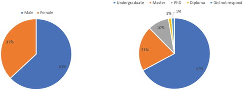
I targeted the subjects who were or had been enrolled in the specific study that teaches finance and/or Brownian motion (e.g., Economics, Finance, Physics, Mathematics and Statistics). Most of them (48 subjects) had participated in at least one economic experiment prior to this experiment. The average payment to the subjects was £8.1 and the average duration of the experiment (including reading the instructions and the payment session) was around one and quarter hours. Communication was prohibited during the experiment. The experimental software was written (mainly by Alfa Ryano) in Python 2.7.

4. Econometric specification

I use maximum likelihood to estimate the parameter of the model—risk aversion (γ), estimating subject by subject. Maximum likelihood requires a specification of the stochastic nature of the data to capture the noise or error in the subjects’ choice (θ_t). I assume this error is independent in every period during trading (t). Since the optimal choice (θ_t*) takes any values, I consider a normal distribution to specify the stochastic story to account for this case. I assume that the choice of θ_t was normally distributed with mean θ_t* (so that there is no bias) and standard deviation ς; I will report s = 1/ς which indicates the precision. My estimation takes into account the difference between the model and the actual as the latter is bounded between 0 and 1—as I have explained above. This strategy is thought as inferring risk aversion from the subjects’ decisions depending on the context of this experiment itself; in which it remains valid to follow the assumption of risk-averse agent as in Nicolosi (2018).¹⁰

Before I turn to the specification of the log-likelihood function, I introduce further notations which will be used in the estimation to create an interval around θ_t since the log-likelihood function is continuous, while the actual choices were discrete, with steps of 0.1 second:

(7) $\begin{array}{c}{\vartheta }_t^{+}={\vartheta }_t+0.005\\ {\vartheta }_t^{-}={\vartheta }_t-0.005\end{array}$(7)

Given these notations, the log-likelihood function finds the probability that θ_t lies within θ_t⁺ and θ_t⁻ for any given γ (risk aversion). Under this specification, the contribution to the likelihood of an observation θ_t is:

(8) $\begin{array}{c}{\vartheta }_t=0\iff \mathrm{\Phi }\left({\vartheta }_t^{+},{\vartheta }_t^{\ast },\frac{1}{s_1}\right)\\ 0<{\vartheta }_t<1\iff \mathrm{\Phi }\left({\vartheta }_t^{+},{\vartheta }_t^{\ast },\frac{1}{s_1}\right)-\mathrm{\Phi }\left({\vartheta }_t^{-},{\vartheta }_t^{\ast },\frac{1}{s_1}\right)\\ {\vartheta }_t=1\iff \mathrm{\Phi }\left({\vartheta }_t^{-},{\vartheta }_t^{\ast },\frac{1}{s_1}\right)\end{array}$(8)

where ɸ is the cdf of a normal distribution with parameters θ_t* (mean) and 1/s₁ (standard deviation) given an observation θ_t. For this specification, I estimate γ₁ (risk aversion) and s₁ (precision).

I also estimate using the average dataset. This is addressed to minimise the noise since the discrete time step (t) is quite fast (0.1 second). By this, I take an average of the dataset on every second, excluding the initial decision which remains as a single data—that is every 10 discrete time step (t). I denote subjects’ choice as θ^¯i in this specification where i is the average discrete time step. Given this specification, the contribution to the likelihood of an observation θ^¯i is:

(9) $\begin{array}{c}{\bar{\vartheta }}_i=0\iff \mathrm{\Phi }\left({\bar{\vartheta }}_i^{+},{\bar{\vartheta }}_i^{\ast },\frac{1}{s_2}\right)\\ 0<{\bar{\vartheta }}_i<1\iff \mathrm{\Phi }\left({\bar{\vartheta }}_i^{+},{\bar{\vartheta }}_i^{\ast },\frac{1}{s_2}\right)-\mathrm{\Phi }\left({\bar{\vartheta }}_i^{-},{\bar{\vartheta }}_i^{\ast },\frac{1}{s_2}\right)\\ {\bar{\vartheta }}_i=1\iff \mathrm{\Phi }\left({\bar{\vartheta }}_i^{-},{\bar{\vartheta }}_i^{\ast },\frac{1}{s_2}\right)\end{array}$(9)

where θ^¯i⁺ = θ^¯i + 0.005 and θ^¯i⁻ = θ^¯i—0.005. Let me call these two specifications as Nicolosi 1, following the specification in Equation (8)(8) $\begin{array}{c}{\vartheta }_t=0\iff \mathrm{\Phi }\left({\vartheta }_t^{+},{\vartheta }_t^{\ast },\frac{1}{s_1}\right)\\ 0<{\vartheta }_t<1\iff \mathrm{\Phi }\left({\vartheta }_t^{+},{\vartheta }_t^{\ast },\frac{1}{s_1}\right)-\mathrm{\Phi }\left({\vartheta }_t^{-},{\vartheta }_t^{\ast },\frac{1}{s_1}\right)\\ {\vartheta }_t=1\iff \mathrm{\Phi }\left({\vartheta }_t^{-},{\vartheta }_t^{\ast },\frac{1}{s_1}\right)\end{array}$(8) , and Nicolosi 2, following the specification as in Equation (9)(9) $\begin{array}{c}{\bar{\vartheta }}_i=0\iff \mathrm{\Phi }\left({\bar{\vartheta }}_i^{+},{\bar{\vartheta }}_i^{\ast },\frac{1}{s_2}\right)\\ 0<{\bar{\vartheta }}_i<1\iff \mathrm{\Phi }\left({\bar{\vartheta }}_i^{+},{\bar{\vartheta }}_i^{\ast },\frac{1}{s_2}\right)-\mathrm{\Phi }\left({\bar{\vartheta }}_i^{-},{\bar{\vartheta }}_i^{\ast },\frac{1}{s_2}\right)\\ {\bar{\vartheta }}_i=1\iff \mathrm{\Phi }\left({\bar{\vartheta }}_i^{-},{\bar{\vartheta }}_i^{\ast },\frac{1}{s_2}\right)\end{array}$(9) . As with previous specification, I estimate γ₂ (risk aversion) and s₂ (precision) in this specification.

One may think of other stochastic assumptions to underlie estimation. For example, I could use a beta distribution to specify the stochastic of the subjects’ choices since they are bounded between 0 and 1. However, I start simple in this paper with a normal distribution specification.

To give a proper assessment to Nicolosi’s optimal strategy, I fit the data additionally assuming both random and risk-neutral choices. The former (random choice) assumes that the choice of θ_t is random following a uniform distribution; that every allocation decision is equally likely to occur. The latter (risk-neutral choice) assumes that the choice of θ_t follows risk-neutral behaviour. Theoretically, the risk neutrality returns either −Inf or Inf, depending on the asset price change. Here I assume that θ_t is 1 if the asset price goes up, otherwise 0 if the asset price goes down. Note crucially, neither of these alternatives involves parameter risk aversion γ.

Again I consider a normal distribution to specify the stochastic story for both random and risk-neutral choices. I also estimate using both all observations and the average dataset. The contribution to the log-likelihood for these specifications adopts Equations (8)(8) $\begin{array}{c}{\vartheta }_t=0\iff \mathrm{\Phi }\left({\vartheta }_t^{+},{\vartheta }_t^{\ast },\frac{1}{s_1}\right)\\ 0<{\vartheta }_t<1\iff \mathrm{\Phi }\left({\vartheta }_t^{+},{\vartheta }_t^{\ast },\frac{1}{s_1}\right)-\mathrm{\Phi }\left({\vartheta }_t^{-},{\vartheta }_t^{\ast },\frac{1}{s_1}\right)\\ {\vartheta }_t=1\iff \mathrm{\Phi }\left({\vartheta }_t^{-},{\vartheta }_t^{\ast },\frac{1}{s_1}\right)\end{array}$(8) and (9(9) $\begin{array}{c}{\bar{\vartheta }}_i=0\iff \mathrm{\Phi }\left({\bar{\vartheta }}_i^{+},{\bar{\vartheta }}_i^{\ast },\frac{1}{s_2}\right)\\ 0<{\bar{\vartheta }}_i<1\iff \mathrm{\Phi }\left({\bar{\vartheta }}_i^{+},{\bar{\vartheta }}_i^{\ast },\frac{1}{s_2}\right)-\mathrm{\Phi }\left({\bar{\vartheta }}_i^{-},{\bar{\vartheta }}_i^{\ast },\frac{1}{s_2}\right)\\ {\bar{\vartheta }}_i=1\iff \mathrm{\Phi }\left({\bar{\vartheta }}_i^{-},{\bar{\vartheta }}_i^{\ast },\frac{1}{s_2}\right)\end{array}$(9) ) as appropriate. For these specifications, let me call random choice specification as Random 1 (for the all-observation estimation) and Random 2 (for the average-dataset estimation), and Risk Neutral 1 (for the all-observation estimation) and Risk Neutral 2 (for the average-dataset estimation) for risk-neutral choice.¹¹

5. Results and analyses

One main purpose of this paper is how well the optimal strategy of Nicolosi (2018) explains the subjects’ choice compared to other strategies (random and risk-neutral choices). The analyses for this purpose use all observations and average dataset from the real experiment. The former sees 1,801 decisions while the latter sees 181 decisions in each problem for each subject. However, the risk-neutral choice will see 1,800 and 180 decisions respectively, excluding the initial decision, since it is drawn following the realisation of the price change.

Additionally, I develop a simple strategy from a regression model using variables in Nicolosi (2018). This is a simplification of the theory as in Equation (6)(6) $\begin{array}{c}{\vartheta }_t^{\ast }={\vartheta }^M+\frac{{\beta }_m}{W_t^{\ast }}\left(-\frac{1}{\gamma }{C}_2\left(t\right)\mathrm{N}\left(d_2\left(t,{\xi }_t\right)\right)+\left(\frac{\beta }{{\beta }_m}-\frac{1}{\gamma }\right)C_3\left(t\right){\xi }_t^{-\beta /{\beta }_m}\mathrm{\Phi }\left(d_3\left(t,{\xi }_t\right)\right)+\right.\\ \left.\frac{C_1\left(t\right){\xi }_t^{-1/\gamma }{e}^{-0.5d_1{\left(t,{\xi }_t\right)}^2}}{X\sqrt{2\pi \left(T-t\right)}}+\frac{C_2\left(t\right)e^{-0.5d_2{\left(t,{\xi }_t\right)}^2}}{X\sqrt{2\pi \left(T-t\right)}}+\frac{C_3\left(t\right){\xi }_t^{-\beta /{\beta }_m}{e}^{-0.5d_3{\left(t,{\xi }_t\right)}^2}}{X\sqrt{2\pi \left(T-t\right)}}\right)\end{array}$(6) ; hereinafter referred to as Simple 1 (for the all-observation estimation) and Simple 2 (for the average-dataset estimation). As previously, I compare Nicolosi’s optimal strategy and this simple strategy given the estimated risk aversion γ from both the all-observation and average-dataset estimations.

Before going on the main analyses, I estimate the individual risk aversion and precision in Nicolosi 1 and Nicolosi 2, which can be found in Figures 2 and 3.

Figure 2. Estimated individual risk aversion and precision in Nicolosi 1.

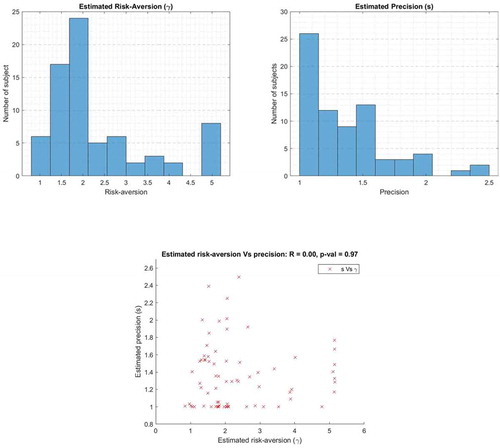
Figure 3. Estimated individual risk aversion and precision in Nicolosi 2.

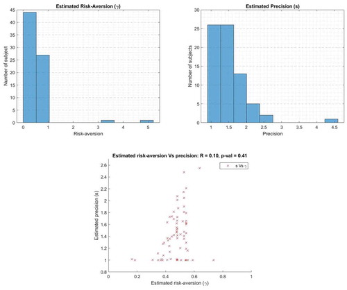
The results between both estimates show that estimate in Nicolosi 2 returns less risk-averse and higher precision on average than that of estimates in Nicolosi 1.¹² This can be a further point of interest, but I take this merely as a consequence of using different approach since the main purpose of this study is to test the empirical validity of Nicolosi’s optimal strategy.

The estimated risk aversion then is used to compute the individual final portfolio values (W_T* as in Equation (3)(3) $W_T^{\ast }=\left\{\left[I\left(\frac{{\lambda }^{\ast }{\xi }_T}{\alpha }\right)-K\right]\frac{1}{\alpha }+Y_T\right\}{\mathrm{I}}_{\left\{{\xi }_T\le \hat{\xi }\right\}}$(3) ) across all problems. It should be the case that following the optimal strategy (W_t*) in each t < T will return a better final portfolio value than that of the final benchmark value given the estimated risk aversion. There are 730 portfolios at maturity in total from 10 problems across 73 subjects. Figure 4 shows comparisons of the optimal portfolio (W_T*) and the benchmark values (Y_T) at maturity across all problems in both Nicolosi 1 and 2.

Figure 4. The optimal portfolio (W_T*) vs the benchmark (Y_T) at maturity given the estimated risk aversion in Nicolosi 1 and Nicolosi 2.

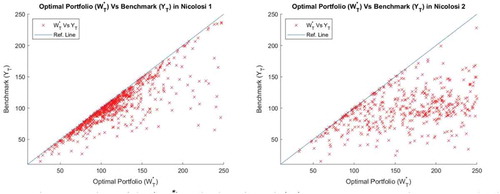
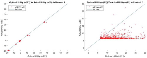
Results from Nicolosi 1 show that all of the final optimal portfolio values (730 portfolios) are better than that of the final benchmark values; meanwhile results from Nicolosi 2 show that 711 final optimal portfolio values (97.4% of the total) are better than that of the final benchmark values given the individual estimated risk aversion. This shows that following the optimal strategy of Nicolosi (in every t < T) is highly likely to end up with both payments (fixed and variable payments). In addition, the optimal portfolios return the higher utility than that of the actual portfolios—as shown in Figure 5.¹³ This is surely not surprising.

Figure 5. Optimal utility (u(Π*)) vs actual utility (u(Π*)) given the estimated risk aversion in Nicolosi 1 and Nicolosi 2.

5.1. Nicolosi’s optimal strategy vs random and risk-neutral strategies

Now we move on to the first comparison between Nicolosi’s optimal strategy and the random and risk-neutral strategies. The concern is to find the best fitting strategy as the explanation of the individual behaviour in selecting the portfolio allocation between the asset and the money account with Nicolosi’s optimal strategy as the subject to test. I measure the goodness-of-fit by maximising the log-likelihood function, as specified in the Equations (8)(8) $\begin{array}{c}{\vartheta }_t=0\iff \mathrm{\Phi }\left({\vartheta }_t^{+},{\vartheta }_t^{\ast },\frac{1}{s_1}\right)\\ 0<{\vartheta }_t<1\iff \mathrm{\Phi }\left({\vartheta }_t^{+},{\vartheta }_t^{\ast },\frac{1}{s_1}\right)-\mathrm{\Phi }\left({\vartheta }_t^{-},{\vartheta }_t^{\ast },\frac{1}{s_1}\right)\\ {\vartheta }_t=1\iff \mathrm{\Phi }\left({\vartheta }_t^{-},{\vartheta }_t^{\ast },\frac{1}{s_1}\right)\end{array}$(8) and (9(9) $\begin{array}{c}{\bar{\vartheta }}_i=0\iff \mathrm{\Phi }\left({\bar{\vartheta }}_i^{+},{\bar{\vartheta }}_i^{\ast },\frac{1}{s_2}\right)\\ 0<{\bar{\vartheta }}_i<1\iff \mathrm{\Phi }\left({\bar{\vartheta }}_i^{+},{\bar{\vartheta }}_i^{\ast },\frac{1}{s_2}\right)-\mathrm{\Phi }\left({\bar{\vartheta }}_i^{-},{\bar{\vartheta }}_i^{\ast },\frac{1}{s_2}\right)\\ {\bar{\vartheta }}_i=1\iff \mathrm{\Phi }\left({\bar{\vartheta }}_i^{-},{\bar{\vartheta }}_i^{\ast },\frac{1}{s_2}\right)\end{array}$(9) ), but we need to correct the maximised log-likelihood for the number of parameters in each specification—Nicolosi’s optimal strategy has two estimated parameters while each of the random and risk-neutral choices has one estimated parameter. In particular, I simulate 100 times of the decisions in each problem to generate the dataset for both random choices (Random 1 and 2), then take its average log-likelihood.¹⁴

I use the Akaike Information Criterion (AIC) as the measure of the goodness-of-fit to find the best explanation for each subject. The details of the judgment can be seen in Appendix D and E. With the all-observation estimation—between Nicolosi 1, Random 1 and Risk Neutral 1—of all 73 subjects, 49 subjects are better explained with Risk Neutral 1 while the other 24 subjects are better explained with Nicolosi 1; Random 1 is always the worst. Nevertheless, with the average dataset estimation, 40 subjects are better explained with Nicolosi 2 while the other 33 subjects are better explained with Risk Neutral 2; Random 2 remains the worst. This finding obviously shows that subjects did not randomise their choice in allocating their portfolio—that they followed some specific strategies for this. In particular, averaging the dataset improves the goodness-of-fit of Nicolosi’s optimal strategy. This may be the evidence that subjects somehow follow the optimal strategy as in Nicolosi’s optimal strategy but having difficulties to be as precise as the theory.

So far it is obvious that the subjects did not randomise their choices, and that following the optimal strategy is highly likely to end up with a better portfolio than that of the benchmark. As it also has shown, Nicolosi’s optimal strategy receives the most empirical support on the average level. Nevertheless, the subjects might find it difficult to follow the optimal strategy of Nicolosi, which involves sophisticated dynamic programming, given his/her risk aversion—calculating and implementing as precise as the optimal strategy. Results from the estimated precision show that the subjects’ choices are noisy compared to the optimal strategy in both Nicolosi 1 and 2; with average estimated precisions are 1.3556 (or standard deviation 0.7377) and 1.4763 (or standard deviation 0.6774) respectively. However, they must respond to some variables shown on the screen to determine their choice.

5.2. Nicolosi’s optimal strategy vs the simple strategy

Building on the previous results, I try to explore the determinants of the subjects’ choice in a simple way using a regression model. Following Nicolosi, the portfolio allocation in the asset (θ_t) should not be constant, as in the Merton’s strategy (θ^M = β_m/γ), when the managed portfolio value is lower than that of the benchmark during trading in order to increase the chance to beat the benchmark at maturity. In particular, θ_t tends to be low, during trading, when the portfolio value (W_t) is higher than that of the benchmark (Y_t), vice versa. So I involve the difference between the managed portfolio and the benchmark (W_t − Y_t) in the regression model; I denote this as ∆_t. In addition, I also involve the asset price (S_t) and the benchmark value (Y_t) since they were shown to the subjects in the experimental interface—I denote θ^¯, S^¯, Y^¯ and ∆^¯ for variables used in Simple 2. The regression results from Simple 1 and Simple 2 are as follows¹⁵:

(10) ${\vartheta }_t=\underset{\left(0.129\right)}{43.649}-\underset{\left(0.005\right)\ast }{0.041S_t}+\underset{\left(0.002\right)\ast }{0.115Y_t}-\underset{\left(0.002\right)\ast }{0.008{\mathrm{\Delta }}_t}$(10)

(11) ${\bar{\vartheta }}_i=\underset{\left(0.401\right)\ast }{43.642}-\underset{\left(0.017\right)\ast \ast }{0.042{\bar{S}}_i}+\underset{\left(0.007\right)\ast }{0.115{\bar{Y}}_i}-\underset{\left(0.004\right)\ast \ast \ast }{0.008{\bar{\mathrm{\Delta }}}_i}$(11)

I use percentage values for θ, t is time step and i is average time step. Overall results from both regression model above show that all independent variables are significant in determining the subjects’ choice—the signs of the independent variables are identical. Both the asset price and the difference between the managed portfolio and the benchmark have a negative effect on the subjects’ choice, meanwhile, the value of the benchmark has a positive effect on the subjects’ choice. These results are sensible and intuitive. Overall, subjects tended to buy the asset when its price was low and to sell the asset when its price was high; to some extent, it is commonly known as “buy low, sell high” strategy. This strategy is possibly the most famous adage in making profits from an asset market. Moreover, subjects tended to hold the asset as they saw the benchmark value was high. Lastly, subjects were consistent with the theoretical prediction in which they were unlikely to hold the asset when their portfolio value was relatively far above the benchmark.

Building on the regression results, I then run the regression model individually using the same structure as in Equations (10)(10) ${\vartheta }_t=\underset{\left(0.129\right)}{43.649}-\underset{\left(0.005\right)\ast }{0.041S_t}+\underset{\left(0.002\right)\ast }{0.115Y_t}-\underset{\left(0.002\right)\ast }{0.008{\mathrm{\Delta }}_t}$(10) and (11(11) ${\bar{\vartheta }}_i=\underset{\left(0.401\right)\ast }{43.642}-\underset{\left(0.017\right)\ast \ast }{0.042{\bar{S}}_i}+\underset{\left(0.007\right)\ast }{0.115{\bar{Y}}_i}-\underset{\left(0.004\right)\ast \ast \ast }{0.008{\bar{\mathrm{\Delta }}}_i}$(11) ). This is to give a comparison of which model to have a better explanation for each subject between Nicolosi’s optimal strategy and the simple strategy using their measure of the goodness-of-fit; I compare between Nicolosi 1 and Simple 1, and between Nicolosi 2 and Simple 2. Since the models have different specifications, hence different degree of freedom, I calculate the AIC to correct for differing degrees of freedom.¹⁶ I compare them and have a conclusion accordingly for each subject.

Results from the two estimation procedures (using all observations and the average dataset) produce a slightly different AIC conclusion. With the all-observation estimation, 37 subjects are better explained with Nicolosi’s optimal strategy; 36 subjects are better explained with the simple strategy. Meanwhile, with the average-dataset estimation, 36 subjects are better explained with Nicolosi’s optimal strategy; 37 subjects are better with the simple strategy. The details of the judgment can be seen in Appendix F.

6. Discussion and conclusion

This paper examines Nicolosi (2018) by investigating the subjects’ behaviour in order to follow the optimal strategy of Nicolosi in a controlled lab-experiment. Subjects act as if they are the hedge fund manager who takes a responsibility to manage the investor’s funds. The manager agrees on a contract, determined by the investor, who pays the manager with a two-term payment: the fixed payment and the variable payment, where the variable payment is a share-based on the over-performance with respect to the specific benchmark.

I follow Nicolosi’s design in which there are two markets for the manager to invest: the asset market and the money market. The asset price follows geometric Brownian motion and subjects were aware of all parameters used in the experiment. However, there are non-consequential and consequential differences in the experimental setup from the theoretical design. The former relates to the computer limitation to implement the continuous time in generating the asset price, hence I use the discrete approximation to the continuous time with an increment of 0.1 second. The latter restricts the maximum portfolio allocation between the asset and the money account, and that the subjects are not allowed to either borrow and lend money. This is addressed to prevent the subjects from a negative payoff from short-selling since it may have an unlimited loss.

To give a proper assessment of the empirical validity of Nicolosi (2018), I compare its optimal choice, given the estimated subjects’ risk aversion, with two alternative strategies. First, I compare the optimal strategy of Nicolosi with random and risk-neutral choices. The random choice generates θ (portfolio allocation in the asset market) randomly following a normal distribution while the risk-neutral choice generates θ as if the subject was a risk-neutral agent; put everything on the asset if the asset price goes up, otherwise nothing if the asset price goes down. Second, I compare Nicolosi’s optimal strategy with the simple strategy, developed using a regression model. One obvious conclusion from the first assessment is that the subjects did not randomise their choice. They followed some specific strategies to maximise their utility from the experiment. Of all subjects, 24 subjects are better explained with Nicolosi’s optimal strategy while the other 49 subjects are better explained with risk-neutral choice using all the observations. We get a different conclusion if we use the average dataset. Of all subjects, 40 subjects are better explained with Nicolosi’s optimal strategy; the other 33 subjects are better explained with the risk-neutral choice.

Building on the previous results, I then develop a regression model to provide the simple strategy in which the subjects may plausibly have followed. With this simple strategy, one tends to hold the asset when its price is low and to sell the asset when its price is high. In addition, one manages its portfolio value depending on the benchmark value and the difference between the managed portfolio and the benchmark. I compare Nicolosi’s optimal strategy with this simple strategy individually—as with the previous analysis. The comparison sees that 37 subjects are better explained with Nicolosi’s optimal strategy, 36 others are better explained with the simple strategy, using all observations. If we use the average dataset, we get slightly different results: of all subjects, 36 subjects are better explained with Nicolosi’s optimal strategy, while 37 others are better explained with the simple strategy.

Although the optimal strategy of Nicolosi ensures a high possibility to end up with both fixed and variable payments, hence the maximum utility, the subjects found it difficult to follow. As it has shown, the subjects’ choices are noisy compared with the optimal strategy. One may argue that the subjects could have more precise computation if they were well accommodated in the experiment since Nicolosi’s optimal strategy involves sophisticated dynamic programming. For example, we could ask the subject to specify their own strategy to be implemented during trading at the beginning of each problem, and they are free to adjust their strategy at any time. Will it improve the empirical validity of the theory? I may not think so because it depends on how subjects understand the random process in the asset price, hence determining the benchmark value.

Alternatively, we could go further with other models within similar substantial framework of Nicolosi’s optimal strategy. Among these are Nicolosi et al. (2018) and Herzel and Nicolosi (2019). Both provide the optimal solution for the fund manager, similar to Nicolosi (2018), who invests in one riskless asset and several risky assets. However the former assumes that there is no fixed payment, instead the manager is compensated with implicit incentives as shown in Chevalier and Ellison (1997). By this the asset under management is multiplied if the manager performs well due to the inflow in the investor’s funds, otherwise a part of the asset under management is withdrawn. Other possibility is to model the subject’ choice assuming one preference function within either risk or ambiguity frameworks as shown in He and Zhou (2011) and Ahn et al. (2014), though they do not take into account the payment scheme for the fund manager; but they are not restricted only for the risk-averse agent case. Nevertheless, the optimal choice of Nicolosi (2018) receives strong empirical support in explaining the subjects’ behaviour. In addition, subjects follow the intuitive prediction of Nicolosi’s optimal strategy where the difference between the managed portfolio and the benchmark determines the subjects’ choice.

Acknowledgements

I am thankful to John Hey, Marco Nicolosi, and participants at Gama ICEB 2019 and the 4^th International ICNDBM Conference on New Directions in Business, Management, Finance and Economics for helpful comments and feedback. This paper was funded by Indonesia Endowment Fund for Education (Ref: S-4294/LPDP.3/2015). All errors and omissions are solely mine.

Additional information

Funding

This work was supported by the Indonesia Endowment Fund for Education [Ref: S-4294/LPDP.3/2015].

Notes on contributors

Yudistira Permana

I am a staff at Vocational College, Universitas Gadjah Mada. I hold PhD in Economics from the University of York. My research interests are in Behavioural Economics and Experimental Economics and I have been actively conducting a laboratory experiment, particularly, in individual decision making under risk and under uncertainty. This paper tries to provide the empirical findings of the portfolio strategies where the theory can well-predict human complex thinking and behaviour in the particular setting. In the wider context, it should bring this study into a further exploration on why and how some fund managers may fail to manage the investor’s funds.

Notes

1. This benchmark can be either fixed or variable. The fixed benchmark usually is the expected return from the investment funds whereas the variable benchmark usually is the portfolio value at maturity following the investor’s portfolio allocation choice.

2. One may also refer this to as the “investment planning horizon”.

3. Despite this assumption, there may be various implementation to be taken for the case of under-performance considering that the investor pays a relatively high amount of payment for the manager. For example, a percentage deduction to the fixed payment depending on the magnitude of the under-performance.

4. Black-Scholes setting has following assumptions: a) there are two types of market, the asset market (risky) and the money market (risk-free), b) asset pays no dividend and there is no transaction cost in the market, c) asset price reflects all information in the asset market, d) asset price is exogenous to all agents, e) it is possible to borrow and lend cash at riskless rate as well as doing short-selling, f) the asset price change is random with known parameters, and g) it is possible to buy and to sell asset at any time. This assumption is important in the model in order to draw stochasticity of the asset price.

5. Wiener process (V_t) has the following properties: a) it is continuous, b) its change process is independent of the previous values, c) its increment process follows N(0, d_t), d) V₀ = 0.

6. See Appendix A for the specification of CRRA utility function.

7. State price density contains important information on the behaviour and expectations of the market (Hardle & Hlavka, 2009). It follows a log-normal distribution in the Black-Scholes setting.

8. Equation (2)(2) $\underset{W_T}{max}E\left[u\left(\alpha {\left(W_T-Y_T\right)}^{+}+K\right)\right]s.t.E\left[\frac{{\xi }_T}{{\xi }_0}{W}_T\right]=W_0$(2) is the implication of the martingale approach used in the model which decomposes a dynamic optimization problem $\underset{\vartheta }{max}E\left[u\left(\alpha {\left(W_T-Y_T\right)}^{+}+K\right)\right]$ s.t. W_t into a static optimisation problem as in Equation (2)(2) $\underset{W_T}{max}E\left[u\left(\alpha {\left(W_T-Y_T\right)}^{+}+K\right)\right]s.t.E\left[\frac{{\xi }_T}{{\xi }_0}{W}_T\right]=W_0$(2) . This determines the optimal condition at maturity. This approach was notably developed by Pliska (1986), Karatzas et al. (1987), and Cox and Huang (1989) among others.

9. See Appendix C for the parameters used in the experiment.

10. One alternative is to have a separate experiment to elicit subjects’ risk aversion and calibrate only those risk-averse agents with Nicolosi’s optimal strategy. However Nicolosi (2018) does not say anything about this in which one needs to check if the agent has to be risk averse to enter the game and that inferring risk aversion from the subjects’ decisions remains valid (see Zhou and Hey (2018) for this issue).

11. I use pattersearch routine in Matlab to maximise the log-likelihood function in all specifications.

12. The average estimated risk aversion in Nicolosi 1 is 2.3353 compared to 0.5778 from the result in Nicolosi 2. Meanwhile, the average estimated precision in Nicolosi 1 is 1.3556 compared to 1.4763 from the result in Nicolosi 2; with θ_t is bounded between 0 and 1 whereas θ_t* is unbounded.

13. This sees 535 optimal portfolios (73.29% of the total) returns the better utility than that from the actual portfolios from results in Nicolosi 1; and 665 optimal portfolios (91.1% of the total) returns the better utility than that of the actual portfolios from results in Nicolosi 2.

14. The procedures for this are: i) draw the decisions in each problem using uniform distribution (to create values between 0 and 1) for 100 times, ii) fit the simulated decisions using a normal distribution (as in Equations (8) and (9)) to compute the likelihood, iii) take the average log-likelihood in each problem.

15. I use a simple linear procedure in both regression models. Standard errors are in parentheses and *, **, *** denote the significance at 1%, 5%, and 10% respectively. All coefficients are jointly not equal to zero in both regression model. Adjusted R² in both models are 0.0094 and 0.0097 respectively, and the number of observations is 1,314,730 and 132,130 respectively.

16. The AIC is given by 2 k—2LL, where k is the number of estimated parameters and LL is the log-likelihood.

Appendices

Appendix A.

Specification of CRRA utility function

Nicolosi (2018) assumes that the manager is utility maximiser specified with CRRA utility function. It can be written as:

$CRRA:u\left(x\right)=\frac{x^{1-\gamma }}{1-\gamma };\begin{array}{cc}\gamma >0& \gamma \ne 1\end{array}$

The manager is assumed to be strictly risk-averse and the function is undefined when γ = 1. However I apply CRRA utility function so it is able to accommodate when γ = 1 as follows:

$CRRA:u\left(x\right)=\left\{\begin{array}{c}\frac{x^{1-\gamma }}{1-\gamma };\gamma \ne 1\\ log\left(x\right);\gamma =1\end{array}\right.$

Appendix B.

Definitions to Equation (6)(6) $\begin{array}{c}{\vartheta }_t^{\ast }={\vartheta }^M+\frac{{\beta }_m}{W_t^{\ast }}\left(-\frac{1}{\gamma }{C}_2\left(t\right)\mathrm{N}\left(d_2\left(t,{\xi }_t\right)\right)+\left(\frac{\beta }{{\beta }_m}-\frac{1}{\gamma }\right)C_3\left(t\right){\xi }_t^{-\beta /{\beta }_m}\mathrm{\Phi }\left(d_3\left(t,{\xi }_t\right)\right)+\right.\\ \left.\frac{C_1\left(t\right){\xi }_t^{-1/\gamma }{e}^{-0.5d_1{\left(t,{\xi }_t\right)}^2}}{X\sqrt{2\pi \left(T-t\right)}}+\frac{C_2\left(t\right)e^{-0.5d_2{\left(t,{\xi }_t\right)}^2}}{X\sqrt{2\pi \left(T-t\right)}}+\frac{C_3\left(t\right){\xi }_t^{-\beta /{\beta }_m}{e}^{-0.5d_3{\left(t,{\xi }_t\right)}^2}}{X\sqrt{2\pi \left(T-t\right)}}\right)\end{array}$(6)

Solution in Equation (6)(6) $\begin{array}{c}{\vartheta }_t^{\ast }={\vartheta }^M+\frac{{\beta }_m}{W_t^{\ast }}\left(-\frac{1}{\gamma }{C}_2\left(t\right)\mathrm{N}\left(d_2\left(t,{\xi }_t\right)\right)+\left(\frac{\beta }{{\beta }_m}-\frac{1}{\gamma }\right)C_3\left(t\right){\xi }_t^{-\beta /{\beta }_m}\mathrm{\Phi }\left(d_3\left(t,{\xi }_t\right)\right)+\right.\\ \left.\frac{C_1\left(t\right){\xi }_t^{-1/\gamma }{e}^{-0.5d_1{\left(t,{\xi }_t\right)}^2}}{X\sqrt{2\pi \left(T-t\right)}}+\frac{C_2\left(t\right)e^{-0.5d_2{\left(t,{\xi }_t\right)}^2}}{X\sqrt{2\pi \left(T-t\right)}}+\frac{C_3\left(t\right){\xi }_t^{-\beta /{\beta }_m}{e}^{-0.5d_3{\left(t,{\xi }_t\right)}^2}}{X\sqrt{2\pi \left(T-t\right)}}\right)\end{array}$(6) contains some components (C₁, C₂, C₃, d₁, d₂ and d₃) where they are defined as follows:

$C_1\left(t\right)=\frac{1}{\alpha }{\left(\frac{{\lambda }^{\ast }}{\alpha }\right)}^{-\frac{1}{\gamma }}exp\left[\left(\frac{1}{\gamma }-1\right)\left(r+\frac{1}{2\gamma }{X}^2\right)\left(T-t\right)\right]$

$C_2\left(t\right)=-\frac{K}{\alpha }exp\left[-r\left(T-t\right)\right]$$C_3\left(t\right)=Y_0{A}_{T}exp\left[\left(\frac{\beta }{{\beta }_m}-1\right)\left(r+\frac{1}{2}\beta \alpha X\right)\left(T-t\right)\right]$

$d_1\left(t,{\xi }_t\right)=\frac{ln\left(\frac{\hat{\xi }}{{\xi }_t}\right)+\left(r-\frac{1}{2}{X}^2\left(1-\frac{2}{\gamma }\right)\right)\left(T-t\right)}{X\sqrt{T-t}}$

$d_2\left(t,{\xi }_t\right)=\frac{ln\left(\frac{\hat{\xi }}{{\xi }_t}\right)+\left(r-\frac{1}{2}{X}^2\right)\left(T-t\right)}{X\sqrt{T-t}}$

$d_3\left(t,{\xi }_t\right)=\frac{ln\left(\frac{\hat{\xi }}{{\xi }_t}\right)+\left(r-\frac{1}{2}{X}^2\left(1-\frac{2\beta }{{\beta }_m}\right)\right)\left(T-t\right)}{X\sqrt{T-t}}$

$A_T=exp\left[\left(r+\frac{1}{2}\beta \sigma X-\frac{1}{2}{\beta }^2{\sigma }^2-r\frac{\beta \sigma }{X}\right)T\right]$

Appendix C.

Parameters used in the experiment

Table

W0	K	a	b	r	m	s	bm
100	0.1	0.2	95	0	0.1	0.25	1.6
100	0.1	0.5	30	0	0.1	0.5	0.4
100	0.1	0.5	15	0	0.1	0.75	0.18
100	0.1	0.1	95	0	0.25	0.25	4
100	0.1	0.3	90	0	0.25	0.5	1
100	0.1	0.4	40	0	0.25	0.75	0.44
100	0.1	0.1	95	0	0.5	0.25	8
100	0.1	0.2	95	0	0.5	0.5	2
100	0.1	0.4	75	0	0.5	0.75	0.89
100	0.1	0.3	95	0	0.75	0.75	1.33

Appendix D.

Individual AIC of Nicolosi’s optimal strategy vs random and risk-neutral strategies from the all-observation estimation

Table

Sub.	Nicolosi 1	Random 1	Risk Neutral 1	Judgment
1	198,321.246	210,458.42	196,036.112	Risk Neutral 1
2	94,621.670	103,252.13	95,907.756	Nicolosi 1
3	197,009.678	206,736.15	191,808.286	Risk Neutral 1
4	192,582.322	205,440.70	189,739.869	Risk Neutral 1
5	122,903.085	131,323.40	119,387.990	Risk Neutral 1
6	189,562.792	203,599.82	189,052.356	Risk Neutral 1
7	84,860.704	94,743.10	99,462.459	Nicolosi 1
8	186,540.242	197,489.72	183,558.288	Risk Neutral 1
9	182,607.437	206,393.14	195,904.024	Nicolosi 1
10	106,135.443	114,638.24	115,009.369	Nicolosi 1
11	196,790.120	210,550.01	193,273.823	Risk Neutral 1
12	54,509.687	63,318.91	59,471.648	Nicolosi 1
13	152,116.133	161,483.96	153,503.171	Nicolosi 1
14	194,862.244	211,418.61	193,953.201	Risk Neutral 1
15	186,890.991	204,993.00	191,504.509	Nicolosi 1
16	189,016.232	197,130.47	181,871.617	Risk Neutral 1
17	148,867.582	156,670.82	147,838.409	Risk Neutral 1
18	176,018.071	144,099.70	138,768.587	Risk Neutral 1
19	163,426.340	171,948.40	161,666.209	Risk Neutral 1
20	189,294.637	197,458.22	184,832.636	Risk Neutral 1
21	160,497.587	168,868.88	155,350.027	Risk Neutral 1
22	186,078.435	197,709.35	183,769.752	Risk Neutral 1
23	170,643.478	179,437.87	170,967.209	Nicolosi 1
24	51,079.834	60,661.36	54,270.308	Nicolosi 1
25	187,165.955	199,075.21	186,916.125	Risk Neutral 1
26	126,078.497	134,849.94	116,499.274	Risk Neutral 1
27	151,085.506	159,730.07	145,798.463	Risk Neutral 1
28	175,190.721	183,009.93	169,266.254	Risk Neutral 1
29	157,320.343	165,790.83	146,924.193	Risk Neutral 1
30	190,712.679	201,154.21	186,811.810	Risk Neutral 1
31	157,683.899	165,125.00	153,422.846	Risk Neutral 1
32	188,010.084	209,725.21	195,939.363	Nicolosi 1
33	171,356.837	178,758.00	163,075.761	Risk Neutral 1
34	180,645.237	197,379.75	186,878.163	Nicolosi 1
35	148,606.352	157,244.16	144,722.103	Risk Neutral 1
36	149,326.154	160,138.15	154,822.340	Nicolosi 1
37	115,501.088	124,699.35	114,856.663	Risk Neutral 1
38	164,300.775	170,770.96	163,826.794	Risk Neutral 1
39	105,318.745	113,154.80	105,075.899	Risk Neutral 1
40	193,010.105	205,181.35	191,613.115	Risk Neutral 1
41	193,079.490	204,731.75	191,125.544	Risk Neutral 1
42	102,158.038	111,409.66	102,023.025	Risk Neutral 1
43	191,534.105	206,604.65	192,924.714	Nicolosi 1
44	100,711.684	109,670.23	96,066.439	Risk Neutral 1
45	189,579.881	196,953.22	180,829.065	Risk Neutral 1
46	194,783.214	211,692.26	194,219.174	Risk Neutral 1
47	182,924.555	194,544.88	183,673.065	Nicolosi 1
48	116,701.608	125,449.08	113,366.554	Risk Neutral 1
49	124,055.332	132,704.73	119,136.480	Risk Neutral 1
50	164,785.441	173,582.61	161,453.783	Risk Neutral 1
51	161,217.997	171,680.07	163,137.731	Nicolosi 1
52	191,179.743	200,443.71	182,570.474	Risk Neutral 1
53	154,667.291	163,779.70	158,500.161	Nicolosi 1
54	180,204.121	188,702.36	176,427.731	Risk Neutral 1
55	128,189.903	136,756.42	130,924.244	Nicolosi 1
56	135,654.533	143,500.28	138,158.201	Nicolosi 1
57	170,254.851	183,409.56	175,979.028	Nicolosi 1
58	191,571.075	210,099.06	195,161.530	Nicolosi 1
59	130,256.125	139,254.34	119,740.229	Risk Neutral 1
60	190,167.843	201,295.98	190,014.183	Risk Neutral 1
61	202,235.566	212,381.62	197,466.484	Risk Neutral 1
62	172,044.525	181,493.87	170,416.059	Risk Neutral 1
63	90,625.379	99,469.07	94,595.255	Nicolosi 1
64	207,332.067	216,244.32	199,915.193	Risk Neutral 1
65	109,043.874	117,602.46	112,917.040	Nicolosi 1
66	194,080.405	210,981.87	197,334.587	Nicolosi 1
67	193,908.536	206,246.64	193,144.819	Risk Neutral 1
68	187,425.745	197,164.77	182,043.057	Risk Neutral 1
69	94,374.381	104,505.78	86,862.585	Risk Neutral 1
70	199,755.572	209,608.82	193,689.952	Risk Neutral 1
71	174,579.674	207,351.28	196,189.365	Nicolosi 1
72	127,173.519	135,185.75	126,914.538	Risk Neutral 1
73	191,689.817	200,140.16	185,153.444	Risk Neutral 1

Appendix E.

Individual AIC of Nicolosi’s optimal strategy vs random and risk-neutral strategies from the average-dataset estimation

Table

Sub.	Nicolosi 2	Random 2	Risk Neutral 2	Judgment
1	19,645.443	21,276.915	19,707.556	Nicolosi 2
2	10,308.974	11,193.485	10,451.865	Nicolosi 2
3	19,654.644	20,824.513	19,323.457	Risk Neutral 2
4	19,110.957	20,640.147	19,102.646	Risk Neutral 2
5	12,721.576	13,839.208	12,584.114	Risk Neutral 2
6	18,881.490	20,317.375	18,992.737	Nicolosi 2
7	9,073.263	10,184.285	10,598.342	Nicolosi 2
8	18,432.750	19,969.587	18,455.694	Nicolosi 2
9	18,211.662	20,770.769	19,736.161	Nicolosi 2
10	10,910.544	11,754.292	11,842.976	Nicolosi 2
11	18,562.476	21,137.327	19,419.260	Nicolosi 2
12	7,072.808	8,048.429	7,463.668	Nicolosi 2
13	15,570.811	16,717.952	15,900.244	Nicolosi 2
14	19,276.702	21,393.806	19,518.378	Nicolosi 2
15	18,478.606	20,689.534	19,321.530	Nicolosi 2
16	18,698.295	19,906.145	18,266.338	Risk Neutral 2
17	15,867.467	16,935.297	15,956.145	Nicolosi 2
18	14,487.021	15,402.747	14,690.872	Nicolosi 2
19	16,512.099	17,603.555	16,428.442	Risk Neutral 2
20	19,139.755	20,234.076	18,857.811	Risk Neutral 2
21	16,221.765	17,298.968	15,863.659	Risk Neutral 2
22	18,577.961	19,904.596	18,524.010	Risk Neutral 2
23	17,297.021	18,426.621	17,560.452	Nicolosi 2
24	6,858.525	7,942.105	7,112.858	Nicolosi 2
25	18,743.614	20,199.865	18,818.953	Nicolosi 2
26	12,183.404	13,464.854	11,740.719	Risk Neutral 2
27	15,094.474	15,998.310	14,710.935	Risk Neutral 2
28	17,693.703	18,735.166	17,281.467	Risk Neutral 2
29	15,456.541	16,566.724	14,783.131	Risk Neutral 2
30	18,890.308	20,424.891	18,803.754	Risk Neutral 2
31	15,895.487	16,899.731	15,689.552	Risk Neutral 2
32	18,526.775	21,013.143	19,693.844	Nicolosi 2
33	17,015.108	18,033.247	16,477.604	Risk Neutral 2
34	18,015.064	19,712.386	18,891.320	Nicolosi 2
35	15,146.999	16,297.791	14,817.561	Risk Neutral 2
36	15,168.377	16,386.540	15,804.205	Nicolosi 2
37	11,896.929	13,007.154	11,961.519	Nicolosi 2
38	16,989.139	17,973.530	16,897.985	Risk Neutral 2
39	11,219.657	11,878.243	11,340.596	Nicolosi 2
40	19,240.664	20,644.909	19,315.266	Nicolosi 2
41	19,068.611	20,668.949	19,148.219	Nicolosi 2
42	10,929.215	11,753.924	10,954.997	Nicolosi 2
43	19,046.644	20,809.280	19,378.574	Nicolosi 2
44	10,393.924	11,427.371	10,090.863	Risk Neutral 2
45	18,747.958	19,808.119	18,217.787	Risk Neutral 2
46	19,584.232	21,074.995	19,521.625	Risk Neutral 2
47	18,272.897	19,689.729	18,539.222	Nicolosi 2
48	12,098.261	13,148.804	11,856.479	Risk Neutral 2
49	12,740.073	13,788.326	12,463.929	Risk Neutral 2
50	16,569.828	17,559.341	16,499.363	Risk Neutral 2
51	16,448.717	17,641.751	16,770.022	Nicolosi 2
52	18,932.483	20,124.124	18,280.755	Risk Neutral 2
53	15,785.945	16,783.599	16,236.848	Nicolosi 2
54	18,267.852	19,138.988	18,006.249	Risk Neutral 2
55	13,141.490	14,093.093	13,500.656	Nicolosi 2
56	14,167.084	15,102.149	14,434.206	Nicolosi 2
57	16,924.950	18,543.676	17,803.038	Nicolosi 2
58	19,007.689	21,019.668	19,604.083	Nicolosi 2
59	12,676.044	14,087.649	12,218.915	Risk Neutral 2
60	19,037.041	20,432.582	19,166.922	Nicolosi 2
61	20,077.660	21,307.750	19,884.740	Risk Neutral 2
62	17,388.911	18,508.138	17,368.394	Risk Neutral 2
63	10,421.870	11,311.637	10,742.597	Nicolosi 2
64	20,533.681	21,696.645	20,089.477	Risk Neutral 2
65	11,727.217	12,763.400	12,039.345	Nicolosi 2
66	19,164.185	21,168.094	19,823.653	Nicolosi 2
67	19,276.851	20,707.507	19,318.071	Nicolosi 2
68	18,828.910	19,929.108	18,379.339	Risk Neutral 2
69	10,400.811	11,497.089	9,721.980	Risk Neutral 2
70	19,798.275	21,168.097	19,464.585	Risk Neutral 2
71	16,337.286	20,801.975	19,652.329	Nicolosi 2
72	13,006.015	13,986.488	13,040.748	Nicolosi 2
73	19,224.107	20,539.412	18,838.633	Risk Neutral 2

Appendix F.

Individual AIC of Nicolosi’s optimal strategy vs the simple strategy from the all-observation and average-dataset estimations

Table

Sub.	Nicolosi 1	Simple 1	Judgment	Nicolosi 2	Simple 2	Judgment
1	198,321.246	174,453.096	Simple 1	19,645.443	17,455.645	Simple 2
2	94,621.670	187,219.239	Nicolosi 1	10,308.974	18,728.059	Nicolosi 2
3	197,009.678	177,602.827	Simple 1	19,654.644	17,758.940	Simple 2
4	192,582.322	166,821.787	Simple 1	19,110.957	16,733.459	Simple 2
5	122,903.085	182,955.881	Nicolosi 1	12,721.576	18,304.908	Nicolosi 2
6	189,562.792	168,015.790	Simple 1	18,881.490	16,891.658	Simple 2
7	84,860.704	171,150.393	Nicolosi 1	9,073.263	17,002.175	Nicolosi 2
8	186,540.242	171,222.098	Simple 1	18,432.750	17,215.338	Simple 2
9	182,607.437	166,307.909	Simple 1	18,211.662	16,608.700	Simple 2
10	106,135.443	182,277.380	Nicolosi 1	10,910.544	18,228.427	Nicolosi 2
11	196,790.120	157,968.120	Simple 1	18,562.476	15,843.093	Simple 2
12	54,509.687	189,229.569	Nicolosi 1	7,072.808	18,861.851	Nicolosi 2
13	152,116.133	174,479.333	Nicolosi 1	15,570.811	17,457.335	Nicolosi 2
14	194,862.244	149,449.397	Simple 1	19,276.702	15,026.829	Simple 2
15	186,890.991	140,797.022	Simple 1	18,478.606	14,131.838	Simple 2
16	189,016.232	170,370.559	Simple 1	18,698.295	17,123.570	Simple 2
17	148,867.582	182,301.089	Nicolosi 1	15,867.467	18,154.031	Nicolosi 2
18	176,018.071	188,021.265	Nicolosi 1	14,487.021	18,768.873	Nicolosi 2
19	163,426.340	163,742.014	Nicolosi 1	16,512.099	16,425.107	Simple 2
20	189,294.637	182,459.465	Simple 1	19,139.755	18,084.611	Simple 2
21	160,497.587	180,933.397	Nicolosi 1	16,221.765	18,095.145	Nicolosi 2
22	186,078.435	172,963.107	Simple 1	18,577.961	17,361.759	Simple 2
23	170,643.478	183,885.162	Nicolosi 1	17,297.021	18,371.147	Nicolosi 2
24	51,079.834	189,411.817	Nicolosi 1	6,858.525	18,873.701	Nicolosi 2
25	187,165.955	176,686.211	Simple 1	18,743.614	17,630.047	Simple 2
26	126,078.497	173,352.631	Nicolosi 1	12,183.404	17,410.910	Nicolosi 2
27	151,085.506	180,397.210	Nicolosi 1	15,094.474	18,129.940	Nicolosi 2
28	175,190.721	176,939.549	Nicolosi 1	17,693.703	17,721.956	Nicolosi 2
29	157,320.343	153,376.336	Simple 1	15,456.541	15,409.923	Simple 2
30	190,712.679	170,171.255	Simple 1	18,890.308	17,041.947	Simple 2
31	157,683.899	184,829.529	Nicolosi 1	15,895.487	18,514.293	Nicolosi 2
32	188,010.084	161,722.966	Simple 1	18,526.775	16,250.788	Simple 2
33	171,356.837	166,172.225	Simple 1	17,015.108	16,676.372	Simple 2
34	180,645.237	170,523.007	Simple 1	18,015.064	17,085.953	Simple 2
35	148,606.352	181,124.271	Nicolosi 1	15,146.999	18,123.924	Nicolosi 2
36	149,326.154	173,965.530	Nicolosi 1	15,168.377	17,377.665	Nicolosi 2
37	115,501.088	185,358.890	Nicolosi 1	11,896.929	18,521.134	Nicolosi 2
38	164,300.775	190,106.051	Nicolosi 1	16,989.139	18,786.662	Nicolosi 2
39	105,318.745	188,589.613	Nicolosi 1	11,219.657	18,861.343	Nicolosi 2
40	193,010.105	179,141.643	Simple 1	19,240.664	17,959.728	Simple 2
41	193,079.490	175,035.633	Simple 1	19,068.611	17,448.843	Simple 2
42	102,158.038	187,359.316	Nicolosi 1	10,929.215	18,753.266	Nicolosi 2
43	191,534.105	168,380.417	Simple 1	19,046.644	16,883.941	Simple 2
44	100,711.684	184,714.380	Nicolosi 1	10,393.924	18,524.670	Nicolosi 2
45	189,579.881	156,042.604	Simple 1	18,747.958	15,683.010	Simple 2
46	194,783.214	154,996.682	Simple 1	19,584.232	15,558.910	Simple 2
47	182,924.555	179,923.901	Simple 1	18,272.897	18,060.958	Simple 2
48	116,701.608	188,101.443	Nicolosi 1	12,098.261	18,841.319	Nicolosi 2
49	124,055.332	179,661.868	Nicolosi 1	12,740.073	17,995.199	Nicolosi 2
50	164,785.441	182,127.024	Nicolosi 1	16,569.828	18,263.963	Nicolosi 2
51	161,217.997	180,868.857	Nicolosi 1	16,448.717	18,068.112	Nicolosi 2
52	191,179.743	150,357.056	Simple 1	18,932.483	15,120.175	Simple 2
53	154,667.291	181,851.840	Nicolosi 1	15,785.945	18,154.987	Nicolosi 2
54	180,204.121	176,885.073	Simple 1	18,267.852	17,667.756	Simple 2
55	128,189.903	183,068.355	Nicolosi 1	13,141.490	18,362.161	Nicolosi 2
56	135,654.533	187,990.605	Nicolosi 1	14,167.084	18,768.260	Nicolosi 2
57	170,247.571	177,850.007	Nicolosi 1	16,924.950	17,838.094	Nicolosi 2
58	191,571.075	157,387.741	Simple 1	19,007.689	15,819.855	Simple 2
59	130,256.125	170,843.543	Nicolosi 1	12,676.044	17,157.900	Nicolosi 2
60	190,167.843	183,068.432	Simple 1	19,037.041	18,190.008	Simple 2
61	202,235.566	174,855.835	Simple 1	20,077.660	17,534.646	Simple 2
62	172,044.525	178,631.531	Nicolosi 1	17,388.911	17,846.881	Nicolosi 2
63	90,625.379	186,551.648	Nicolosi 1	10,421.870	18,584.942	Nicolosi 2
64	207,332.067	171,978.988	Simple 1	20,533.681	17,291.396	Simple 2
65	109,043.874	190,880.268	Nicolosi 1	11,727.217	19,066.867	Nicolosi 2
66	194,080.405	164,270.808	Simple 1	19,164.185	16,518.488	Simple 2
67	193,908.536	177,807.706	Simple 1	19,276.851	17,709.987	Simple 2
68	187,425.745	171,412.721	Simple 1	18,828.910	17,112.860	Simple 2
69	94,374.381	185,129.275	Nicolosi 1	10,400.811	18,465.155	Nicolosi 2
70	199,755.572	167,452.215	Simple 1	19,798.275	16,821.980	Simple 2
71	174,579.674	117,201.218	Simple 1	16,337.286	11,732.197	Simple 2
72	127,173.519	186,266.268	Nicolosi 1	13,006.015	18,667.986	Nicolosi 2
73	191,689.817	170,526.544	Simple 1	19,224.107	17,077.428	Simple 2

References

- Ahn, D. S., Choi, S., Gale, D., & Kariv, S. (2014). Estimating ambiguity aversion in a portfolio choice experiment. Quantitative Economics, 125(1), 40–20. https://doi.org/10.3982/QE243
- Browne, S. (1999). Beating a moving target: Optimal portfolio strategies for outperforming a stochastic benchmark. Finance and Stochastics, 3(3), 275–284. https://doi.org/10.1007/s007800050063
- Carpenter, J. N. (2000). Does option compensation increase managerial risk appetite? The Journal of Finance, 55(5), 2311–2331. https://doi.org/10.1111/0022-1082.00288
- Chevalier, J., & Ellison, G. (1997). Risk taking by mutual funds as a response to incentives. The Journal of Political Economy, 105(6), 1167–1200. https://doi.org/10.1086/516389
- Cox, J. C., & Huang, C.-F. (1989). Optimal consumption and portfolio policies when asset prices follow a diffusion process. Journal of Economic Theory, 49(1), 33–83. https://doi.org/10.1016/0022-0531(89)90067-7
- Gabih, A., Grecksch, W., & Richter, M. (2006). Optimal portfolio strategies benchmarking the stock market. Mathematical Methods of Operational Research, 64(2), 211–225. https://doi.org/10.1007/s00186-006-0091-3
- Guasoni, P., & Obloj, J. (2016). The incentives of hedge fund fees and high-water marks. Mathematical Finance, 26(2), 269–295. https://doi.org/10.1111/mafi.12057
- Härdle, W., & Hlávka, Z. (2009). Dynamics of state price densities. Journal of Econometrics, 150(1), 1-15. doi:10.1016/j.jeconom.2009.01.005
- He, X. D., & Zhou, Y. X. (2011). Portfolio choice under cumulative prospect theory: An analytical treatment. Management Science, 57(2), 315–331. https://doi.org/10.1287/mnsc.1100.1269
- Herzel, S., & Nicolosi, M. (2019). Optimal strategies with option compensation under mean reverting returns or volatilities. Computational Management Science, 16(1–2), 47–69. https://doi.org/10.1007/s10287-017-0296-3
- Hildebrand, P. M. (2005). Recent developments in the hedge fund industry. Swiss National Bank Quarterly Bulletin, 23-1(2005), 42–57. https://www.snb.ch/en/mmr/speeches/id/ref_20050204_pmh
- Hodder, J. E., & Jackwerth, J. C. (2007). Incentive contracts and hedge fund management. The Journal of Finance and Quantitative Analysis, 42(4), 811–826. https://doi.org/10.1017/S0022109000003409
- Karatzas, I., Lehoczky, J. P., & Shreve, S. E. (1987). Optimal portfolio and consumption decisions for a small investor on a finite horizon. SIAM Journal on Control and Optimization, 25(6), 1557–1586. https://doi.org/10.1137/0325086
- Merton, R. C. (1969). Lifetime portfolio selection under uncertainty: The continuous-time case. The Review of Economics and Statistics, 51(3), 247–257. https://doi.org/10.2307/1926560
- Merton, R. C. (1971). Optimum consumption and portfolio rules in a continuous-time model. Journal of Economic Theory, 3(4), 373–413. https://doi.org/10.1016/0022-0531(71)90038-X
- Nicolosi, M. (2018). Optimal strategy for a fund manager with option compensation. Decisions in Economics and Finance, 41(1), 1–17. https://doi.org/10.1007/s10203-017-0204-x
- Nicolosi, M., Angelini, F., & Herzel, S. (2018). Portfolio management with benchmark related incentives under mean reverting processes. Annals of Operations Research, 266(1–2), 373–394. https://doi.org/10.1007/s10479-017-2535-y
- Palomino, F., & Prat, A. (2003). Risk taking and optimal contracts for money managers. The RAND Journal of Economics, 34(1), 113–137. https://doi.org/10.2307/3087446
- Panageas, S., & Westerfield, M. M. (2009). High-water marks: High risk appetites? Convex compensation, long horizons, and portfolio choice. The Journal of Finance, 64(1), 1–36. https://doi.org/10.1111/j.1540-6261.2008.01427.x
- Pliska, S. R. (1986). A stochastic calculus model of continuous trading: Optimal portfolios. Mathematics of Operations Research, 11(2), 371–382. https://doi.org/10.1287/moor.11.2.371
- Zhou, W., & Hey, J. (2018). Context matters. Experimental Economics, 21(4), 723–756. https://doi.org/10.1007/s10683-017-9546-z