Analyzing the Railway Network of the Belt and Road Initiative

Abstract

Rail freight has exhibited significant growth within the last decade between Asia and Europe, especially after the announcement of China’s Belt and Road Initiative in 2013, which consists of seaborne and land routes. Within the latter one, this paper focuses on the railroad network that consists of six major corridors. Using the software AnyLogic (Version 8), we give a macroscopic model designed as a GIS-based discrete-event model of rail freight from China to Germany under existing border control point capacities, eventually providing a general overview toward the classification of different routes and countries and later ranking them according to their criticality index. This criticality index is computed as a product of time variance and the Logistics Performance Index. The former is obtained through various scenario analyses within the paradigm of shortest route and current border control points having constant capacity, but variable number of trains per day. In an attempt to understand the network under stress, the results obtained from this study also establish the need to increase the processing capacity at border control points to maximize the utilizability of this transcontinental railway network. The results show that lower capacity at border control points leads to higher time for trains to reach their destination. Stakeholders who are actively seeking to expand their Belt and Road Initiative investment or using rail transportation may understand when the network would reach peak performance and what measures could help to accomplish its maximum efficiency.

Keywords:

• Belt and Road Initiative
• simulation
• freight
• railways
• capacity
• border

PUBLIC INTEREST STATEMENT

The Belt and Road Initiative was introduced by China back in 2013, which consists of seaborne and land routes including railroad. In an attempt to better understand the railroad network, we developed a simulation model to analyze the changes to journey of picking different routes. Our results show that lower capacity at border control points leads to higher time for trains to reach their destination. Stakeholders who are actively seeking to expand their Belt and Road Initiative investment or using rail transportation may understand when the network would reach peak performance and what measures could help to accomplish its maximum efficiency. Furthermore, forming two categories of countries, i.e., southern and northern corridor countries, our analyses yield that Russia, Kazakhstan, Poland, and Belarus are the most important countries in the northern corridor, whereas Turkey is the most important country in the southern corridor.

1. Introduction

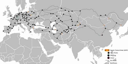
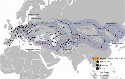
The Belt and Road Initiative (BRI) was introduced by President Xi Jinping of China (PRC) in September and October of 2013 during his visits to Kazakhstan and Indonesia. The initiative consisted of two parts: “Silk Road Economic Belt (SREB)” and “21st Century Maritime Silk Road (MSR)” (Blanchard & Flint, 2017). SREB, primarily composed of six economic corridors, as illustrated in Figure 1, aimed to link Europe with China over land via rail and road (Baniya et al., 2019). Each corridor links China with its BRI participant countries in Asia, carving its way to Europe, which previously relied on sea and air (or limited land routes). The MSR as a sea transportation route, despite having critical limitations and issues (see, e.g., Uygun and Jafri (2020)), compliments the mesh of rail network, aimed to further strengthen the supply chain with the wider world by providing additional routing options through the Suez Canal (IRU, 2017). As a massive connectivity plan by the People’s Republic of China, the total cost will be exceeding more than 1 USD trillion and spanning over more than 65 countries. Border connectivity among the member countries to facilitate trade is one of the top priorities of the projects within BRI. It involves the construction of numerous infrastructural projects and trade facilitation agreements (Xu & Herrero, 2017). Its importance for China is also significant by giving the chance for its western region to develop and help diversify its economy and trading routes.

Figure 1. Six corridors and MSR route. Source: (IRU, 2017)

Collectively, BRI is highly relevant for modern supply chains (see, e.g., Güller et al., 2015 and Besenfelder et al., 2013) and has the potential to reshape supply chains (Thürer et al., 2020), especially in sectors where reliable just-in-time (for further explanation, see, e.g., Uygun & Straub, 2013, Kortmann & Uygun, 2007, or Straub et al., 2013 or Uygun et al., 2011) is necessary or for goods with less weight and high value (Ruta et al., 2018). According to a brief by the World Bank Group, a fully realized version of BRI has the capacity to reduce travel time of cargo by up to 12% and increase trade in range of 2.7–9.7% whilst also elevating poverty of 7.6 million people (Freund & Ruta, 2018). Each corridor has its own significance; however, our study will revolve around the southern China-Central Asia-West Asia Economic Corridor (CCWAEC) and the northern corridors New Eurasia Land Bridge Economic Corridor (NELBEC) and China–Mongolia–Russia Economic Corridor (CMREC) due to its growing prominence in rail freight sector (prominently between Europe and China).

The cost of rail freight is about 80% lower than air freight, with only about half the time than sea. The same study compares the cost variation in the last decade between the change in cost and time between the three modes of transportation; extrapolating the cost and time lines reveals that not only the rail freight resides perfectly in between sea and air freight, but also has the capacity to decrease the transit time and costs as the market continues to grow (see Appendix A Figure 18). Air freight rates can never touch as low as the ones for sea or land. Neither can ships travel as fast to be able to deliver the cargo within 8.5–20 days when compared with trains.

According to a study by DSV Panalpina, a generic comparison of 1 FEU (weighing approximately 22,000 kg or 40 ft. container) cost by three modes of transportations between China and Europe reveals that transportation of goods by train is twice as expensive as by ships, but four times as cheap as transport by air (DSV, 2019). Rail transportation is advantageous over air freight due to astounding prices relative to air, especially during the COVID-19 pandemic. The price of cargo per kilogram between Europe and China was about 0.24 USD per kg, in contrast to air freight with 7.33 USD per kg—a stark 2,954.17% difference amidst lack of availability of slots in air freight, as major seaports were closed (Cole, 2020).

In contrast to past, there are regular rail services being run by numerous operators, e.g., CRE, Yu’Xin’Ou, DB Schenker, and DHL, among others. The number of freight trains is expected to increase in coming years, and such has been forecasted by various researchers in academia, GOs, and NGOs. Rail freight in 2016 had about 2.1% share in the overall trade by value, between China and Europe, which is an increase of 1.3% since 2007 (Kosoy, 2018). The increase was the highest at the time of the publication of the article by CSIS (Hillman, 2018). A more recent statistics by Chinese Railways, Belt and Road Portal, shows that the present trains per day (tpd) is already 14 block trains (Wagner et al., 2019). In addition, in 2016 the International Union of Railways (UIC) forecasted an increase of up to about 21 F tpd between the two continents by 2027 at a CAGR of 14.7% (Berger, 2017). According to the BRI Portal, the number of trains (including block trains and others) in 2018 between the two continents was 6,363, which averages to about 17–18 tpd in both directions (BRI Portal, 2019), stating that the potential shift from air and sea might be sooner than expected.

For sustainable growth and continued development of trains, it is important to keep in mind that railways are less flexible as railway systems work in closed loops, linked by a series of processes. Increasing traffic is constraining the railway networks at various locations. These unintended delays due to the lack of harmonization and capacity could result in reduced attractiveness of trains as a mode of transportation (UNECE, 2015). A general understanding is that by improving the logistical situation, e.g., by decreasing the queuing time at border control points (BCPs) with improved workflows (e.g., see in Lyutov et al., 2019) or increasing its efficiency to minimize errors (see, e.g., Lyutov et al., 2021) and decreasing the transhipment transfer process, countries can significantly improve their innovation ecosystems (see, e.g., Reynolds & Uygun, 2018) and overall Logistics Performance Indicator (LPI), a leading ranking by the World Bank, which as a result would translate into its improved international ranking. However, it will also suggest that BCP processing capacity can be a cause of bottleneck in future.

Against the backdrop of this, the capacity limitation problem at BCP (nodes) is suggested to be addressed by this study. These limitations are divided into two categories as physical and nonphysical barriers. Physical barriers occur due to technical reasons such as varied railway systems (NIIAT, 2017), varied gauges (He, 2016), or scarce rolling stocks (Zhang & Schramm, 2018); inadequate or complete lack of infrastructure at a given link or node; and inability of handling a certain capacity or certain objects. Nonphysical obstacles negatively affect the quality of services, e.g., improper handling of cargo, transparency level of procedures, and policies (NIIAT, 2017); inefficient BCP Procedure (ESCAP, 2018) (CAREC, 2018); inconsistent custom regulations (Yan & Filimonov, 2018) (Jakóbowski, et al., 218); border security (Haiquan, 2017) (Islam, et al., 2013); and shipment disparity (Leijen, 2019) (Feng et al., 2020). Apart from that, sustainability aspects, e.g., discussed in Sayyadi & Awasthi, 2018, Sayyadi & Awasthi, 2020, or Dubey et al., 2015, are not considered in this study, although they are relevant to the BRI discussion. But the primary goal of this study is to understand the different corridors in terms of journey time.

2. Literature review

There are several studies on railroad networks that either use discrete-event simulation or analytical modeling, which will be reviewed in this section. Since we address capacity limitations as well, scientific contributions on the capacity of the railroad network are reviewed, too.

Considering capacity in railroad networks, several contributions exist to describe the capacity-related issues.

The way to contextualize the capacity in railways can be dependent on several factors. For example, Burdett and Kozan (2006) define capacity as the highest quantity of trains that can pass through a given bottleneck (node) in a unit of time. Furthermore, absolute capacity is the theoretical capacity, though not always realizable nor is in the best interest due to high probability of collisions. Regardless, they demonstrate that the capacity of the bottleneck node is the actual capacity of the whole network and understanding them is important for long-term strategic planning. They calculate the maximum number of trains via optimization models including heterogeneity and delay times.

Landex (2008) highlights the complexity in explaining the railway capacity as it has evolved over time, in addition, is dependent on the context of the project. He concludes that the capacity consists of parameters such as (1) railway infrastructure, (2) rolling stock, (3) scheduling, (4) processing time, and (5) external factors. The study uses discrete-event simulation to design a mesopic model for strategic capacity analysis via SCAN.

Abril et al. (2008) explain four concepts of capacity, i.e., theoretical capacity, practical capacity, used capacity and available capacity. In addition, he explains various methods (namely analytical, optimizing, and simulation method) through which railway capacity can be determined and how different parameters like speed, heterogeneity,¹ and train stops can affect the overall capacity. Arbil also concluded that analytical methods are a good starting point, but for advanced study, optimizing and simulation should be a better alternative, depending on the environment of the system.

Sameni et al. (2011) highlight that railway node capacity is its ability to generate profit and is also dependent on various dynamic factors like train length, service quality heterogeneity, among others. Their simulation conducted on bulk and intermodal trains through the Berkeley Simulation Software over a 100-mile section concluded that the profitability of railway node is highly dependent on the train number per day and heterogeneity.

Pouryousef et al. (2015), based on more than 50 studies in the United States and Europe, concluded that in the United States the concept and methodologies vary significantly relative to the one in Europe, who are more consistent in their capacity studies and techniques. Similarly, timetabling is of more importance in Europe with focus on automation. Heterogeneity of trains is greater in Europe. The study also highlights three main methods to analyze capacity: (1) analytical, (2) simulation, and (c) combination of analytical simulation, which benefits from higher flexibility.

Apart from that dynamic simulation models, mainly discrete-event simulation models were developed and used to better understand issues in railroad networks.

With respect to modeling and simulation, the planning horizon, as discussed in detail by Velde (1999), plays an important role in determining the method and approach one puts in designing the model. For example, for strategic forecasting the use of a macroscopic model that aggregates various processes into one (nodes location, speed between nodes, capacity per day of nodes, type of node, etc.) is helpful, whereas for operations planning a microscopic model with a higher level of detail (agent and resources interaction, resulting in individual behavior) makes more sense, as discussed in Benjamin et al. (1998), e.g., by considering timetables, train heterogeneity, line numbers, individual nodes, signaling system, permissible speed through various smaller junctions, yard location, etc. Macroscopic modeling is usually employed to keep the resolution smaller where a timetable is of least concern at macroscopic level or when data for detailed analysis is simply not available (Mattsson, 2007). Apart from that, there are mesoscopic models that provide a hybrid approach incorporating average fluctuations of microscopic and macroscopic models. For example, entities are modeled individually; the interaction abstraction level is broader relative to microscopic models (Koch & Tolujew, 2013). Marinov et al. (2013) explain the upsides and downsides of each level of model, i.e., macroscopic, mesoscopic, and microscopic, in more detail.

Lindfeldt (2015) uses discrete-event simulation by RailSys and TigerSim to macroscopically analyze the capacity and effect of congestion in double-track railways. The level of detail is within the boundaries of Sweden, incorporating various parameters like heterogeneity, timetables, and distance between nodes and number of trains in the network.

Border control points (BCPs) are special nodes in the railway network where the trains cross countries, and depending on the relationship with the neighboring country will undergo a series of processes (e.g., custom controls, inspections, change of gauge, coupling–decoupling, quarantine, etc.); queuing is also eminent and depends on terminal’s processing capacity. For example, Dimitrov (2011) uses discrete-event simulation to analyze BCP through General Purpose Simulation System (GPSS). He developed three scenarios to analyze the queuing (waiting time) based on server theory working around the clock. Each two servers represent the flow of materials from the origin country and arrival country. His analysis gives a good representation of a relationship of queuing to be served and waiting time, hence revealing a direct link to the capacity constraint of BCP.

Heshmati et al. (2016) use agent-based modeling (on NetLogo) where individual entities are modeled as agents with different internal states and behaviors that change upon interaction with other agents or based on conditions (Güller et al., 2018), (Güller et al., 2013). Heshmati et al. (2016) try to optimize rail–rail transhipment terminals (RRTTs) for gantry cranes’ slot allocation based on availability of railcars awaiting to be processed for an assigned destination. This study highlights the capacity constraints of gantry cranes as one of the most important reasons for shipment delays at terminals and BCP.

Isik et al. (2017) point out that improving LPI is of great importance; and one way to do so is by decreasing the queuing time at the BCP (case study of Kapikule, Turkey BCP). They use discrete-event simulation with ARENA software to describe various processes in series to highlight the bottlenecks causing most of the delays.

Lu et al. (2004) give a brief overview of complexities of railway network in the context of Alameda Corridor. The complexities are even greater when the railways pass through multiple metropolitan areas. Their discrete-event simulation model considers different nodes and links with specific speed for each link in conjunction with their acceleration and deceleration. The model proposes an algorithm for dispatching, which otherwise is manually done by a dispatcher, often resulting in deadlocks.

Woroniuk and Marinov (2013) use discrete-event simulation in ARENA to analyze three different scenarios of train and station interaction—trains representing agents, whereas stations representing as servers (service area). The model is FIFO based; hence, queuing increases the delays when trains exceed the capacity of servers (station), thus, increasing their utilization. His results conclude that the freight routes are performing undercapacity, and therefore, the utilization of line can be further increased by gaining more market share.

Huang et al. (2018) use discrete-event simulation to analyze rail line utilization as a function of speed, eventually estimating the delay-induced energy consumption in China. Their study highlights the scheduling problem as the major cause of delay in Beijing to Yizhuang Metro Line leading to increased train interactions at terminals. The study also pointed out an interesting finding that a delay of 31.79 s in a subsystem causes more than 4,000 s of delays in the system. Therefore, more energy is wasted.

In addition to dynamic simulation models, analytical models were also developed related to railroad issues.

Cichenski et al. (2016) use mathematical modeling (mixed integer linear programming) to crack the terminal scheduling problem and reduce the time to transfer containers between two trains. Their approach takes into account various parameters like distance between the tracks, horizontal and vertical movement of the crane, number of available tracks, and relative position of trains among others, to assign trains into bundles for faster processing, which helps to reduce the train processing time.

Dessouky and Leachman (1995) explain various reasons for train delays and why analytical methods are insufficient to account for the complex procedures leading to further delays at the upstream side. They divide their study in single and double tracks, while using SLAM II Simulation Language to provide analysis of relative delays based on routing option.

Bababeika et al. (2017) use time–space network flow model (analytical model) implemented via General Algebraic Modelling System (GAMS) to find vulnerable links in the rail network. They use a scenario-based approach to evaluate the number of links failing between nodes and how timetabling may have to use rescheduling and rerouting.

Summing up, existing studies mainly highlight the individual processes taking place at nodes or focus on microscopic modeling and simulation to increase the efficiencies of railway terminals. So, much research is at the microscopic level that focuses on operations. However, a long-term strategic view to see the BCPs’ bottlenecks impeding the timely delivery is still missing. While it is a feasible way to increase the efficiency of internal processes of a node, the effect of these processes leading to the impact on total journey time of trains has not been done at large, especially not for those that relate to BRI, trains, and BCPs along the way for strategic planning. There are also various studies that are still ongoing on the feasibility of the different routes under different conditions, whilst countries are racing to develop their internal infrastructure to promote greater trade through railway. There is also a lack of studies that relate the novel rail freight and capacity limitation of BCPs along the Euro-Asian Transport Linkages (EATL) routes at strategic level. Therefore, the purpose of this paper is to fill this gap and serve as a first step for future research through modeling and simulation of the BRI railway network.

3. Methodology

AnyLogic (version 8.5.2) was selected as the simulation platform of choice that supports conventional and hybrid approach for modeling at any abstraction level, while also allowing individual entity behaviors that can interact with each other (discrete-event and agent-based modeling). The flexibility offered in AnyLogic in the form of a multimethod or hybrid approach is utilized to perform this study, where agents (trains) are placed in an open Geographic Information System (GIS) space and a network of routes is traced. The trains are bound to only use the network, and discrete-event modeling is used to explain individual processes at selected nodes (departure city, arrival city, and selected BCPs) within the network. The software also supports model optimization, sensitivity analyses, parameter variations, and Monte Carlo simulations. To measure the results, three key performance indicators (KPIs) are chosen:

1. Queue lengths (Q_l): Used to analyze the amount of trains that can pile up at the BCP under certain conditions. Observing the maximum and mean number of trains through the BCP will give us a good metrics of the processability of the BCPs.

2. Queue time (Q_t): Train handling capacity of the BCPs can affect the time a train may spend (in days) waiting to be processed in queue where serving is based on FIFO. Each BCP has a certain processing limit per day and the waiting time will help us understand the amount of time a train may spend in queue if more than necessary arrive.

3. Journey time (J_t): Train handling capacity of the BCPs can affect the time a train may spend (in days) waiting to be processed where the rule is FIFO. Each BCP has a certain processing limit per day and the waiting time will help us understand the amount of time a train may spend in queue if more than necessary arrive.

The routes for trains between Europe and China have a certain degree of flexibility depending on the availability of empty slots, traffic condition, and mutual agreement by BRI participant countries; ofttimes the choice is on the rail operators or consigner—some routes are more utilized than others, e.g., Berger (2017), MERICS (2018), Jakóbowski et al. (2018), DHL (2019), and TCITR (2020) provide good overview of a few.

Figure 2. Rail routes network from China to Germany used in this study

These routes are then traced in AnyLogic with the Space Markup toolkit. The data for route mapping is adapted from Reed & Trubetskoy (2019); see Figure 2. Xi’an (China) is assigned as the source of origin of trains and Duisburg (Germany) as the destination.

4. Model design and simulation

In the context of architecture, the model is designed with nine agents (Figure 3) hierarchically connected. Figure 4 shows the model schematics. The input parameters and their values used in the model are given in Table 4 (Appendix A).

Figure 3. List of agents used in this model

Main agent in AnyLogic is the top-level agent consisting of the GIS environment connecting eight other agents. Xi’an is the agent representing the Xi’an city in China where the trains are generated from Rail Library (the process flowchart is shown in Appendix A Figure 19). The city of Duisburg (in Germany) contains trains arrival process where trains undergo decoupling processes and are eventually terminated at Duisburg (see Appendix A Figure 20). Scenario 1 (Route_0), Scenario 2 (Route_1), Scenario 3 (Route_2), and Scenario 4 (Route_3) are agents containing process flowcharts of each scenario (see Appendix A Figures21–24, respectively).

Figure 4. Model diagram extracted from AnyLogic Main Agent

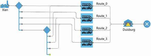
It is to be noted that the model is readjusted for Scenario 5 in a way that it can use common BCP processes for the network, as a result avoiding independent calculations (Appendix A Figure 25).

5. Scenario analysis

Five scenarios were developed, touching upon almost 35 countries, where each scenario has its own subcase. One can understand that in near future train traffic could be 20 tpd (in 1–3 years) and mid to far future train traffic may possibly be in the range of 40–100 tpd (in 5 or more years). These scenarios will shed light on the best route in the network (shortest path) under current border conditions.

5.1. Scenario 1

The routes in Scenario 1 go through western China where it connects to Kazakhstan through two BCPs: (1) Alashankou–Dostyk and (2) Khorgos–Altynkol. Following Kazakhstan, the trains enter Russia from where they pass through Moscow before entering Belarus. At Brest in Belarus they undergo change of gauge. Conventionally, the trains go through Poland to reach Germany. However, more recently some companies² have opted to utilize the Lithuania, Kaliningrad Oblast to Poland to enter Germany to overcome delay problem at Brest–Małaszewicze BCP (due to capacity limitation). Figure 5 gives a high-level description of the routes, whereas Figure 26 (Appendix B) gives a cartographic view. In addition, the Scenario 1 is divided into three possibilities or cases.

Figure 5. Flowchart of the train route from China to Germany, Scenario 1

• Case I: Trains coming from China to Germany go along Alashankou–Dostyk (China–Kazakhstan) and Brest–Małaszewicze (Belarus–Poland) until they reach Duisburg, Germany.

• Case II: Cargo trains are randomly distributed with 50% probability to choose between Khorgos–Altynkol (China–Kazakhstan) and Alashankou–Dostyk (China–Kazakhstan) to prevent congestion at both BCPs, eventually reaching Duisburg, Germany, through Brest–Małaszewicze.

• Case III: This is the extension of Case II; however, in this case the trains can either take only Brest–Małaszewicze (Case III) or both Brest–Małaszewicze and/or Kaliningrad Oblast (Case III–Kaliningrad) depending on the queue length—only when there is no queue, trains will opt at Minsk to take the former route to reach Duisburg, Germany.

Under the current conditions of BCPs in this route, it is apparent that, as the number of trains increases, the journey time J_t increases too. However, when the congestion parameter condition is enabled at the European side (by diverting the excess trains toward Kaliningrad Oblast—Russian Territory) J_t decreases significantly, for simulation runs where trains are over 20 per day (see Figure 6). Not surprisingly, when trains are within the processable limits of Brest–Małaszewicze BCP, it serves as the shortest distance to Duisburg, hence providing a 3.33% time advantage over the latter route (compare Case III and Case III–Kaliningrad for 20 tpd). Under full stress of 100 tpd, Kaliningrad provides 23.92% time saving compared to the conventional Brest–Małaszewicze routes, which equates to a saving of about 5.2 days (124.8 h). The difference between Cases I and II shows the time advantage of using two2 BCPs at Kazakhstan simultaneously owing to the increase in the number of trains from already operating at limit of Alashankou–Dostyk BCP—time difference ranges from 9.38% to 13.98% (compare Cases I and II from 20 to 100 trains per day). Cases II andIII show the highest difference in time, revealing that the Brest–Małaszewicze has capacity limitation problems. Moreover, under most circumstances the trains bound westward from China using this BCP as an entry point to Europe for its gauge change facility.

Figure 6. Average time to complete the journey from Xi’an to Duisburg in Scenario 1

For a detailed variation in queue length and queue times at each BCP on this route, refer to Appendix B Tables 5–7. It can be concluded that in order to maximize the benefit of this route, in view of its growing popularity due to the distance advantage compared to other routes, there is a need for increase in BCP processing capacity in the near future for a sustainable growth. Cases II and III further confirm that increasing the number BCPs or their processing capacity directly influences the journey time J_t owing to increased queue length Q_l and queue time Q_t.

5.2. Scenario 2

In this scenario, trains go through northern China where they enter Mongolia via Erenhot-Zamiin Udd BCP, eventually traveling on the Trans-Mongolian Railway, before joining the Trans-Siberian Railway Network (see Figure 7 and Appendix B Figure 27 for cartographic visualization). Change of gauge also occurs at this BCP, hence a bottleneck in this section often causes significant delays. From Moscow, the trains follow the route as described in Scenario 1 (except traffic will not be diverted at Kaliningrad Oblast because the limiting BCP here is Erenhot-Zamiin Udd BCP).

Figure 7. Flowchart of the train route from China to Germany, Scenario 2

In this case, trains will pass through two BCPs, Erenhot-Zamiin Udd and Brest–Małaszewicze. The reason not to include Kaliningrad Oblast is because the capacity constraint will always be from the former station, i.e., Erenhot-Zamiin Udd. BRI has provided a great chance for Mongolia to take advantage of the growing trade between the two continents. Mongolia provides a shortcut to the traditional Trans-Siberian Railway Network through Ulaanbaatar as the main city connecting China and Russia.

As expected, the number of trains per day is directly proportional to J_t. An increase in 100% trains per day (20 to 100) increases J_t about 74.22%, 42.94%, 30.12%, and 23.57%, respectively (see Figure 8). Comparing the simulation results in Appendix B Table 8, we see that the bottleneck is Erenhot-Zamiin Udd BCP as the leading factor for delays when the same number of trains per day passes in the network, primarily due to its limited processing capacity. As queues happen at a particular node, the subsequent node with higher capacity does not face any queuing.

Figure 8. Average time to complete the journey from Xi’an to Duisburg in Scenario 2

For example, an average of 20 trains per day can lead to an average queue length Q_l of 25.853 trains, equivalent of 1.94 days delay (Q_t) per train until all trains are processed. It can be concluded that for this route to develop the capacity of Erenhot-Zamiin Udd BCP should be increased.

5.3. Scenario 3

Trains going through western China have two options at Harbin city: (1) Route 2a using full length of Trans-Siberian Railway Network from Suifenhe–Pogranichny BCP or (2) Route 2b through Trans-Manchurian Railway before joining Trans-Siberian Railway Network via Manzhouli–Zabaikal’sk at Chita city (see Figure 9). Once trains are on the Trans-Siberian Railway Network, they follow the same path and constraints as in Scenario 1 (Appendix B Figure 28 for cartographic visualization). In addition, Scenario 3 is divided into three possibilities or cases.

Figure 9. Flowchart of the train route from China to Germany, Scenario 3

• Case I: In this case, the effect on the KPI will be measured with condition that trains will use Suifenhe–Pogranichny and Brest–Małaszewicze as the only two BCPs trains can utilize.

• Case II: Here, trains will randomly select between Suifenhe–Pogranichny and Manzhouli–Zabaikal’sk, with a 50% probability, eventually entering Germany through Brest–Małaszewicze.

• Case III: All BCPs with the routes will be fully utilized including the condition of congestion prevention at Brest–Małaszewicze by diverting the trains through Kaliningrad Oblast.

Suifenhe–Pogranichny BCP (has the highest trains per day capacity within the Euro-Asian Transport Linkages EATL routes) is known as a traditional train route carrying cargo from China’s eastern region to Europe over the Trans-Siberian Railway Network. Case I shows that relying solely upon the Suifenhe–Pogranichny BCP up to 20 trains per day can serve the purpose; however, if the number increases to 40 or more, the route starts experiencing capacity limitations and significantly longer journey times (Appendix B, Table 9). However, when 50% trains are diverted to Manzhouli–Zabaikal’sk BCP (in Case II, when compared to Case I), the average J_t varies in range of 5% (100 trains) to 9% (20 trains). The effect of increasing capacity by opening all BCPs as shown in Case III leads to a drastic decrease in overall average J_t.

Figure 10. Average time to complete the journey from Xi’an to Duisburg in Scenario 3

Case III–Kaliningrad offers a better performance in terms of J_t than Case II where only Brest–Małaszewicze BCP is being available—up to almost 50% better performance for higher numbers of trains per day. An interesting fact, due to the heavy queueing at Brest–Małaszewicze, is that the journey time J_t via Kaliningrad is always better under all load profiles, with up to 63% saving in time (equivalent to 5.76 days) when trains discharge rate is 40 per day in Case III. Detailed queue length Q_l and queue time Q_t profiles are shown in Appendix B, Tables 9–11. For Case I, Brest–Małaszewicze BCP shows greater Q_l due to higher capacity of Suifenhe–Pogranichny BCP. The difference between each case grows significantly when trains per day exceed 20 per day. A case-by-case average journey time is shown in Figure 10.

5.4. Scenario 4

In context of China–Europe, the longest route in distance and time to reach Europe is through Bulgaria. For the purpose of this study, Khorgos–Altynkol, Serakhs–Sarakhs, Turkmenbashi–Baku, and Kapikule–Kapitan Andreevo will be included in the study (see Figure 11 and Appendix B Figure 29 for cartographic visualization).

Despite the distance disadvantage, the route holds its importance with its ability to connect China via land to various Central Asian countries including Middle East and provides an alternative to passing through Russia.

Figure 11. Flowchart of the train route from China to Germany, Scenario 4

The model includes two scenarios:

• Case I: Train will go through Iran.

• Case II: Trains will bypass Iran to take Caspian Sea route. Here, change of mode of transportation occurs at Turkmenbashi seaport and then at Baku seaport; from ships to train.

There is also an alternative way that bypasses Uzbekistan, Turkmenistan, and Iran via Caspian Sea from Kazakhstan at Aktau Sea Port and Atyrau Sea Port. However, they are not included in the modeling to avoid sea routes as much as possible by minimizing the distance between two seaports (Turkmenbashi–Baku ferry route provides the shortest disruption in mode of transportation in context of time).

In this case, we will analyze the KPIs in (CCWAEC in depth. As can be seen from the results, the J_t exceeds all other scenarios even at the lowest case of 20 trains per day due to longer distance and more than 2–3 BCPs along the way.

Figure 12. Average time to complete the journey from Xi’an to Duisburg in Scenario 4

Although Cases I and II do not make much of a difference in terms of J_t (0.18–0.5 days at max, see Figure 12) because of loading and unloading procedures (intermodal); even though the distance is reduced by bypassing Iran through the Caspian Sea. The limited capacity of both seaports can be further confirmed by the queue length Q_l and queue time Q_t of Kapikule–Kapitan Andreevo BCP in Tables 12 and 13, where it shows almost no queueing due to queuing at Baku and Turkmenbashi. The maximum queues formed in this route are at Khorgos–Altynkol as the network is stressed with train population. It is also the shortest way in our network (and in reality) to Duisburg.

5.5. Scenario 5

Figure 13. Routes in Scenario 5

Source: Adapted from Reed & Trubetskoy (2019).

Scenario 5 is the combination of all routes in the aforementioned scenarios, utilizing all possible cases with a total of nine BCPs (Figure 13), however, with higher limit of tpd to stress the network under current BCP conditions than the previous scenarios. A submodel is generated in which different routes share similar BCPs (for schematics, see Appendix B Figure 25). All routes are simultaneously being exploited, which will help to identify the ultimate number of freight trains within the existing BCP capacity and therefore help us conclude our understanding. Note that for the purpose of this simulation the case with seaports is not considered (to avoid intermodal transport).

• Case I: In this case, all routes mentioned in the above scenarios would be used.

• Case II: In contrast to Case I, this case will analyze the effect of avoiding low LPI regions.

The average time to complete the journey per train increases with number of trains inserted. However, comparing Cases I and II in Figure 14 the difference lies in a range of 1–10%; Case II is higher than Case I. In contrast, the maximum journey time for both cases varies in each case (see Figure 15). It can be assumed that the overall average time despite incorporating the routes going via Iran in the network does not significantly affect the overall average time. Hence, dispersing the excess train on equal probability through all routes shows that the average time does decrease when routes through Iran are also utilized in conjunction with other.

Figure 14. Mean J_t.

Figure 15. Max J_t.

Greater number of routes (hence more BCPs) leads to greater processing of trains under congestion, resulting in decreased average J_t even under stress. Interestingly, for 20–100 trains per day the maximum J_t in Cases I and II does not show much difference; however at 120– 160 trains per day, the maximum time difference between Cases I and II starts to differ more significantly due to longer distance and capacity constraints, leading to delays by forming large queues, and as a result, arriving at Xi’an later than expected. Although the average time may not show much deviation in both cases under different load profiles, the maximum journey time J_t does. The difference between best scenario and its case reveals that the other routes are evidently longer and more BCP may not necessarily mean better lead time—which means expanding the capacity of exiting BCPs may be a better option. Appendix B Table 14 shows a detailed BCP analysis for Scenario 5.

6. Analysis of simulation

6.1. Ranking the scenarios

Table 1 shows the variation in average journey time J_t under different scenarios conducted.

Table 1. Scenario ranking based on 40 or more tpd—average J_t

Trains/day (load profile)						Points^3
Scenario	20	40	60	80	100
S1: Case III	8.25	9.65	12.44	15.58	19.14	5/5
S3: Case III	10.57	11.99	15.28	17.97	21.41	4/5
S1: Case II	9.6	16.76	23.54	30.68	37.75	2/5
S2	10.24	17.84	25.5	33.18	41	2/5
S1: Case I	10.5	18.76	27.08	35.41	43.88	2/5
S3: Case I	13.92	20.91	28.04	35.18	42.46	1/5
S4: Case II	21.19	37.68	54.18	70.84	87.64	0/5
S4: Case I	21.37	38.01	54.67	71.34	88.14	0/5

The standard deviation is 20.53 days, with a mean of 30.24 days. It can be deduced that under most circumstances the ranking serves as a guideline for which situation is the best amongst all scenarios. It is also evident from various runs and scenario analyses that the majority of BCPs would eventually reach their peak operational capacity.

While keeping 20 days average J_t as the reference point, it can be deduced that S1: Case III receives the highest points, followed by S3: Case III, S1: Case II, and S2. Both cases in Scenario 4 fail to complete the journey within the existing constraints under all circumstances. The J_t results of Scenarios 5 (in Figures 14 and 15) and S1: Case III indicate that using all routes at the same time does increases the network carrying capacity; thus, reaching the failure point (J_t > 20 days) much later (at 120–140 tpd).

6.2. Ranking the countries

Our model is further used to analyze the importance of countries by cutting off the links in the network to-and-from these countries. Based on the result, two categories of countries can be formed due to geological, historical, and development reasons.

• Northern corridor countries (Category 1): Identified by the countries above Caspian Sea (as our anchor point). These countries fall under the shortest path paradigm. It has been noted that this corridor is also the main choice of trains within the network—comprising of mainly NELBEC.

• Southern corridor countries (Category 2): The countries that are on east, west, and southern sides of the Caspian Sea. It can be noted that these countries form the greater part of CCWAEC.

Countries will be ranked on the Criticality Index (C.I) defined by Equation (2), which produces a product of two different indicators; percentage variance (PV) and LPI (WBG, 2018).

(i) $PV=\left[\frac{\left(J_t^n-J_t^b\right)}{J_{\mathrm{t}}^b}\right]$(i)

$J_t^n-$new journey time after excluding the country from the simulation

$J_t^b-$original journey time established in our base case

$J_t^b-$ percentage variance in journey time between the new and base case.

(ii) $C.I=LP{I}_{2018}\cdot PV$(ii)

C.I will try to sort the importance of each country with respect to train’s time variation when a country is not a part of the railway network in the model. For example, a network without any Iranian tracks or a situation when Iran’s network is inaccessible. LPI adds another dimension to the result from a global perspective (more on LPI in Appendix B Table 15).

6.3. Northern corridor countries

Base case route: The base case is defined as the route with the shortest distance and least BCPs, and least time under the assumption of no stoppage at any place with an average speed of 50 km/h throughout the journey for a train. The results for the base case led to 8.79 days to cover the distance under the normal assumed condition in the model.

After various iterative experiments of the model, the results yield that Russia, Kazakhstan, Poland, and Belarus are the most important countries in the northern corridor.

Figure 16. Map based on C.I of countries in northern corridor (higher value, higher importance)

.

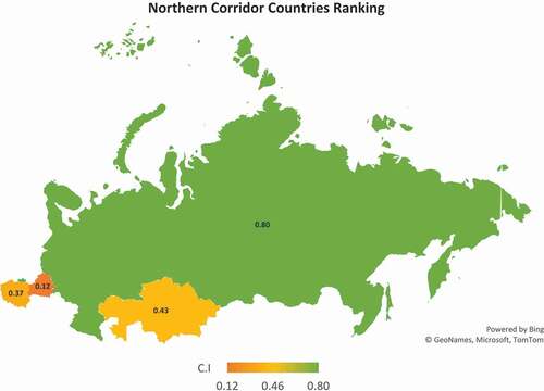
A blockade in one of these will lead to significant delays or a possible collapse of the whole network if other routes are not being used. For example, to reach Europe, blocking Russia leaves trains no other option but to use CCWAEC, which itself is high risk and is seen as a low LPI region. In addition, the delays caused by higher number of BCPs coupled with greater distance along with intermodal transports can lead to unreliable service. The reason for this is the utilization of TSRN; and in case it is not used, then it is unavoidable to cross the Volgograd region of Russia to reach Europe via Ukraine, which is not fully operational due to political reasons. Caspian Sea and Black Sea do help to avoid the Russian region, which puts Kazakhstan and CCWAEC into play, but the present operational challenges due to loading and unloading (from trains to ship and vice versa) cause increased costs. Figure 16 illustrates the results of Table 2. However, the results are dynamic and may change from time to time due to growing number of ongoing projects and various countries competing to be a part of the transit trade. The results can also change based on other factors like propagation of new faster rail links.

Table 2. Critical index of northern corridor countries

Country	% Variance—avg. Jt	LPI	C.I	Ranking
Russia	30	2.69	0.80	1st
Kazakhstan	15	2.77	0.43	2nd
Poland	10	3.50	0.37	3rd
Belarus	5	2.54	0.12	4th

6.4. Southern corridor countries

To meet the desired objective, trains must avoid northern corridor countries for comparison purposes (whenever possible). Hence, this may involve manually steering when needed in addition to travel through the proposed rail links between China, Tajikistan, and Kyrgyzstan through Kashgar (city in Western China).

Base case route: The base case is defined as the route with the shortest distance and least time under the assumption of no stoppage at any place and an average speed of 50 km/h (and 15 km/h for ships over any sea route) throughout the journey for a train. The results for the base case led to 12,307.38 km and time to cover of 10.26 days. Comparing the time variance caused by the change in route yields the following result. The difference between base case of northern corridor and southern corridor countries is 2,815.68 km.

The results obtained from simulation experiment show Turkey’s integral role for the passage into Europe (Table 3). An alternative option through Black Sea (Poti to Constanta) is shorter by distance, but longer in context of J_t due to lesser speed of ships (and other intermodal procedures).

Figure 17. Map based on C.I of sSouthern corridor countries (higher value, higher importance)

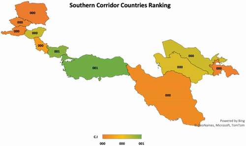
Table 3. Critical index of southern corridor countries

Country	% Variance—avg. Jt	LPI	C.I	Ranking
Turkey	17.02	3.29	0.56	1st
Bulgaria	17.02	3.00	0.51	2nd
Hungary	11.60	3.41	0.40	3rd
Uzbekistan	15.22	2.50	0.38	4th
Turkmenistan	15.22	2.34	0.36	5th
Serbia	4.86	2.83	0.14	6th
Iran	2.70	2.71	0.07	7th
Czechia	0.93	3.62	0.03	8th
Austria	0.83	3.99	0.03	9th
Tajikistan	1.06	2.29	0.02	10th
Poland	0.43	3.50	0.02	11th

Iran faces the same situation (i.e., the alternative option is only the sea route). However, the Caspian Sea is much shorter, hence PV is lesser than that of Turkey. Within the given network, Bulgaria plays a key role as a transit country for the goods coming from Turkey; the other alternative is Black Sea (Poti to Constanta), if Turkey is avoided. Poland is the least important country because of extensive alternate routes available from Czechia, Austria, Switzerland, and France.

C.I is highly influenced by the number of alternative ways and their respective distance when avoiding a country. For example, there are lesser options to avoid Russia, followed by Kazakhstan or Poland; alternative routes are rather longer—coincidently the size of country and C.I show strong correlation; however, this relationship is not present in southern corridor countries, possibly due to intermodal effects. Figure 17 shows a graphical illustration of C.I in the southern corridor.

A singular generic comparison is avoided because the southern corridor is the only possible way as an alternative to the northern corridor with greater number of countries and higher population density—they tend to complement each other. Scenario analyses shed light as to which routes are best in terms of least delay; thus, leading to least J_t. It is concluded that the northern countries primarily in NELBEC provide the best routes in terms of least possible lead time and the shortest distance within the BCPs’ capacity, which is also better developed relative to CCWAEC.

7. Implications and conclusion

Our analysis shows that it is of utmost importance to increase the BCP processing capabilities, but more importantly route diversification for efficient traffic management. And in the context of supply chain security, a breakdown of any part of these routes or nodes could cause long and uncertain lead time on either side of the network. However, any node closure in any of the northern corridor countries would cause the longest delay, and when there is no traffic inflow ability in the northern corridor countries (total blackout), the southern corridor countries could provide another favorable alternative.

We developed five scenarios that were used to shed light on the best route in the network (shortest path) under current border conditions from China to Germany. In Scenario 1 (China, Kazakhstan, Russia, Belarus, [Lithuania, Kaliningrad], Poland, Germany) under the current conditions of BCPs, the journey time increases as the number of trains increases. However, when the congestion parameter condition is enabled at the European side the journey time decreases significantly.

In Scenario 2 (China, Mongolia, Russia, Belarus, Poland, Germany), the number of trains per day is directly proportional to journey time and we see a bottleneck at the Mongolian BCP. So, in order to develop this route, the capacity of this BCP should be increased.

In Scenario 3 (China, Russia, Belarus, [Lithuania, Kaliningrad], Poland, Germany), we see that relying solely upon the eastern Chinese Suifenhe–Pogranichny BCP the route starts experiencing capacity limitations and significantly longer journey times with increasing number. However, when 50% of the trains are diverted to the other Chinese–Russian BCP (Manzhouli–Zabaikal’sk), the average journey time varies in the range of 5% (100 trains) to 9% (20 trains). The effect of increasing capacity by opening all BCPs leads to a drastic decrease in overall average journey time.

In Scenario 4, the route connects China to Germany through various Central Asian and Middle East (Iran, Turkey) countries where one possibility is to cross through Iran or bypass it by taking the Caspian Sea. Although the Caspian route is shorter, it does not make much of a difference in terms of the journey time due to intermodal loading and unloading procedures and capacity limits at the seaports.

In Scenario 5, all routes are simultaneously being exploited with and without low LPI regions. In both cases, the average journey time per train increases with number of trains inserted. Greater number of routes (hence more BCPs) leads to greater processing of trains under congestion, resulting in decreased average journey time even under stress. Interestingly, with increasing number of trains the maximum time difference between both cases starts to differ more significantly due to longer distance and capacity constraints. So, expanding the capacity of exiting BCPs is of importance.

Comparing and ranking those scenarios, we see that the first scenario yields the best results in terms of minimum journey time. In this case, the trains can either take only the Belarus–Poland border or both Belarus–Poland border and/or Kaliningrad depending on the queue length; only when there is no queue, trains will opt at Minsk to take the former route to reach Germany.

We formed two categories of countries, i.e., southern and northern corridor countries, due to geological, historical, and development reasons. After various iterative experiments of the model, the results yield that Russia, Kazakhstan, Poland, and Belarus are the most important countries in the northern corridor. Looking at the southern corridor, Turkey’s integral role for the passage into Europe becomes apparent. An alternative option through Black Sea (Poti to Constanta) is shorter by distance, but longer in the context of the journey time due to lesser speed of ships (and other intermodal procedures).

Summing up, modeling and simulation is an effective technique in understanding the local and global behavior of a dynamic system. Its application on railway networks and its nodes can play a role in optimizing the network to reach its full potential and predict future behavior. In addition, events like the COVID-19 pandemic are testimonials that supply chains are still not resilient enough. For example, closure of important ports, cities, regions, and even countries can lead to economic, social, and political imbalance. Diversification of mode of transportation is equally necessary, and railway is a good alternate mode of transportation between China and other Asian countries to European countries.

There is room for improvement at certain locations like the China–Mongolia border (e.g., Erenhot-Zamiin Udd) as evident in our scenario analysis or Belarus–Poland border (Brest–Małaszewicze). While train speeds are limited by its physical nature, to increase the capacity of goods transfer can be achieved through higher frequency. A higher frequency would mean greater load at BCPs. We showed in this study that, as the number of trains is increasing in the network, congestion at various nodes is growing.

Apart from that, in terms of future research, a thorough literature review, similar to Özgür et al. (2021), can be conducted to get a better overview of all contributions in this context with a focus on showing research gaps. This is important due to the growing popularity of the BRI.

Additional information

Funding

The authors received no direct funding for this research.

Notes on contributors

Yilmaz Uygun

Prof. Dr. Dr.-Ing. Yilmaz Uygun is Professor of Logistics Engineering, Technologies and Processes at Jacobs University Bremen (Germany) and a Research Affiliate at the Industrial Performance Center (IPC) of the Massachusetts Institute of Technology (USA). Prior to this, he worked as Postdoctoral Research Fellow at the IPC. He holds a doctoral degree in engineering from TU Dortmund University/Fraunhofer IML (Germany) and another one in logistics from the University of Duisburg-Essen (Germany). He studied Logistics Engineering at the University of Duisburg-Essen and Industrial Engineering at Südwestfalen University of Applied Sciences (Germany).

Jahanzeb Ahsan

Jahanzeb Ahsan studied Supply Chain Engineering and Management at Jacobs University Bremen (Germany) and graduated with a Master of Science degree in 2020. Prior to this he graduated from The University of Manchester in 2015 with a Bachelor´s degree in Petroleum Engineering. He is currently working as Sales Development Representative at TeamViewer.

Notes

1. Train heterogeneity refers to the mixture of trains like passenger and freight trains. Higher heterogeneity means higher mix of passenger and freight trains and vice versa.

2. Examples: (DHL, 2019) and (DB AG, 2018).

3. Points are based on the rationale that the trains should not take more than 20 days on average to reach the destination, otherwise sea freight would be a better option.

Appendix A

Figure 18. Change in cost (USD/FEU) and time from 2006 to 2017. Data source: Zhang & Schramm, 2018

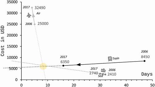
Figure 19. Flowchart of trains being generated at Xi’an (agent), China

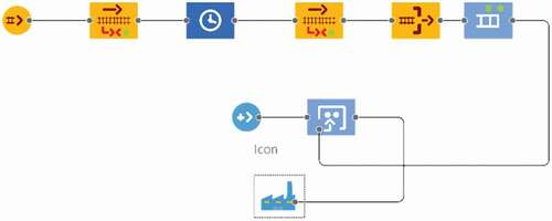
Figure 20. Flowchart of trains arriving in Duisburg, Germany

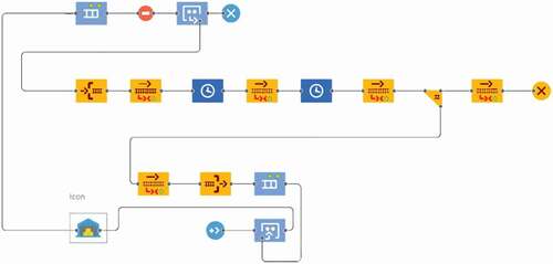
Figure 21. Scenario 1 (Route 0) process flowchart

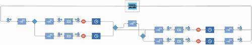
Figure 22. Scenario 2 (Route 1) process flowchart

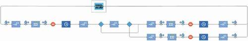
Figure 23. Scenario 3 (Route 2) process flowchart

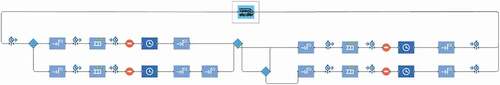
Figure 24. Scenario 4 (Route 3) process flowchart

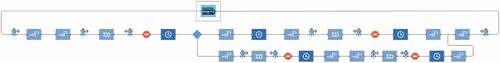
Figure 25. Scenario 5 process flowchart

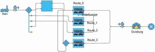
Table 4. Input parameters and their values used in the model

Parameter	Type	Value	Description	Source	Status
BorderDelayAltynkol	Integer	4 h	These parameters define the delay at border caused by reasons other than processing of trains.	Link	Not used
BorderDelayBrest	Integer	10 h		Link	Not used
BorderDelayDostyk	Integer	15 h		Link	Not used
BorderDelayPogranichny	Integer	4 h		Link	Not used
BorderDelaySarakhs	Integer	7 h		Link	Not used
BorderDelayZamiinUdd	Integer	21 h		Link	Not used
BorderDelayZabaikalsk	Integer	12 h		Link	Not used
BorderDelayKapikule	Integer	0		-	Not used
BorderDelayKaliningrad	Integer	0		-	Not used
BorderPortDelayTurkmenbashi	Integer	0		-	Not used
BorderPortDelayBaku	Integer	0		-	Not used
PerDayCapacityAltynkol	Integer	20 tpd	These parameters define the border processing capacity in “trains per day” (tpd).	Link	Used
PerDayCapacityBrest	Integer	14 tpd		Link	Used
PerDayCapacityDostyk	Integer	12 tpd		Link	Used
PerDayCapacityPogranichny	Integer	32 tpd		Link	Used
PerDayCapacitySarakhs	Integer	11 tpd		Link	Used
PerDayCapacityZamiinUdd	Integer	13 tpd		Link	Used
PerDayCapacityZabaikalsk	Integer	14 tpd		Link	Used
PerDayCapacityKapikule	Integer	6 tpd		Link	Used
PerDayCapacityKaliningrad	Integer	24 tpd		Link	Used
PerDayCapacityBaku	Integer	6 tpd		Link	Used
PerDayCapacityTurkmenbashi	Integer	12 tpd		Link	Used
SpeedMongolia	Integer	50 km/h	These parameters define the speed of trains; however for the purpose of this simulation, they are all kept constant, unless otherwise stated.		Used
SpeedTurkey	Integer	50 km/h			Used
SpeedRussia	Integer	50 km/h			Used
SpeedIran	Integer	50 km/h			Used
SpeedEurope	Integer	50 km/h			Used
SpeedChina	Integer	50 km/h			Used
AvgTrain_SpeedCC	Integer	50 km/h			Used
SpeedTurkmenistan	Integer	50 km/h			Used
CaspianShipSpeed	Integer	15–17 km/h		Link	Used
TrainIntervalTime	Integer	9–72 min	-		Used
MaximumTrainsInjected	Integer	200–1600	-		Used
minNoOfCars	Integer	40 rail cars	Number of railcars allowed in Europe through uniform discrete distribution.	Link	Used
maxNoOfCars	Integer	44 rail cars			Used
Route	Integer	0–4	Selects the different routes based on radio selection in main agent (routes 0–3).		Used
Blockvladivostok	Boolean	True or false	Routing parameters.		Used
BlockEurasianLandbridge	Boolean				Used
blockIran	Boolean				Used
blockKZ	Boolean				Used
blockKZandMongolia	Boolean				Used
Congestion_Prevention_Brest	Boolean				Used

Appendix B

Figure 26. Scenario 1 (Route 0) map

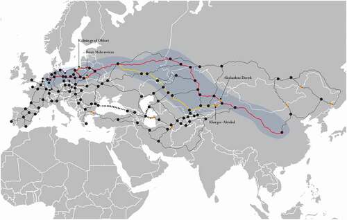
Table 5. Results of different KPIs in Scenario 1, Case I

Trains per day	Alashankou–Dostyk				Brest–Małaszewicze				Journey time
	Ql		Qt		Ql		Qt		Jt
	Avg	Max	Avg	Max	Avg	Max	Avg	Max	Avg	Max
20	28.51	73	2.57	6.4	0	12	0	0	10.5	14.3
40	123.95	268	10.85	24	0	12	0	0	18.76	31.9
60	225.48	468	19.17	41.6	0	12	0	0	27.08	49.5
80	323.49	668	27.5	57.6	0	12	0	0	35.41	65.5
100	423.12	873	35.97	76.8	0	12	0	0	43.88	84.7

Table 6. Results of different KPIs in Scenario 1, Case II

Trains per day	Alashankou–Dostyk				Khorgos–Altynkol				Brest–Małaszewicze				Journey time
	Ql		Qt		Ql		Qt		Ql		Qt		Jt
	Avg	Max	Mean	Max	Avg	Max	Avg	Max	Avg	Max	Avg	Max	Avg	Max
20	0.06	4	0.01	0.4	0	1	0	0.1	14.95	56	1.57	4	9.6	12.3
40	31.2	83	2.91	7.2	0.4	4	0	0.2	82.84	180	7.25	12.8	16.76	27.1
60	69.57	159	6.1	13.6	38.61	99	2.08	5.2	140.97	290	11.51	20.8	23.54	43.1
80	118.48	251	10.21	22.4	199	84.13	4.44	10.4	196.08	382	15.44	28.8	30.68	55.9
100	178.11	379	15.23	32	126.61	287	6.62	14.4	243.7	451	18.77	35.2	37.75	68.7

Table 7. Results of different KPIs in Scenario 1, Case III

Trains per day	Alashankou–Dostyk				Khorgos–Altynkol				Brest–Małaszewicze				Kaliningrad Oblast				Journey time— Brest		Journey time— Kaliningrad
	Ql		Qt		Ql		Qt		Ql		Qt		Ql		Qt		(Case III) Jt		(Case III–Kaliningrad) Jt
	Avg	Max	Avg	Max	Avg	Max	Avg	Max	Avg	Max	Avg	Max	Avg	Max	Avg	Max	Max	Max	Avg	Max
20	0.16	5	0.02	0.5	0	1	0	0.10	0.62	6	0.07	0.5	0	1	0	8.5	8.11	8.6	8.38	8.5
40	29.81	78	2.8	6.8	0.01	2	0	0.1	2.54	18	0.27	1.5	0.27	12	0.03	0.4	10.48	14.7	8.82	11.6
60	70.16	160	6.13	13.6	98	38.23	2.07	5.2	5.91	30	0.54	2.6	0.99	20	0.08	0.3	13.53	21.5	11.34	17
80	116.32	253	10.27	22.4	83.14	196	4.41	10.4	6.47	32	0.57	2.6	1.13	20	0.08	0.3	17.28	30.3	13.87	22
100	175.98	378	15.13	32	128.14	288	6.66	14.4	6.09	32	0.52	2.6	1.123	20	0.08	0.3	21.74	39.9	16.54	29.2

Figure 27. Scenario 2 (Route 1) map

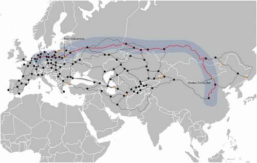
Table 8. Results of different KPIs in Scenario 2

Trains per day	Erenhot-Zamiin Udd				Brest–Małaszewicze				Journey time
	Ql		Qt		Ql		Qt		Jt
	Avg	Max	Avg	Max	Avg	Max	Avg	Max	Avg	Max
20	25.852	63	1.94	5.2	0.63	13	0.07	0.3	10.24	13.4
40	127.53	257	9.56	20.8	0.45	13	0.04	0.3	17.84	29
60	224.93	457	17.25	38.4	0.32	13	0.03	0.3	25.5	46.6
80	326.98	657	24.93	51.2	0.2	13	0.02	0.3	33.18	59.4
100	431.04	863	32.76	70.4	0.2	13	0.02	0.3	41	78.6

Figure 28. Scenario 3 (Route 2) map

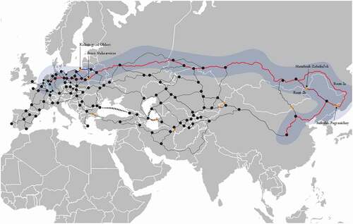
Table 9. Results of different KPIs in Scenario 3, Case I

Trains per day	Suifenhe–Pogranichny				Brest–Małaszewicze				Journey time
	Ql		Qt		Ql		Qt		Jt
	Avg	Max	Avg	Max	Avg	Max	Avg	Max	Avg	Max
20	0	1	0	0.1	11.44	54	1.43	4	13.92	16.4
40	20.444	72	0.77	2.4	78.56	227	7.66	17.6	20.91	31.6
60	104.537	263	3.66	8.8	134.66	341	11.89	25.6	28.04	47.6
80	196.147	458	6.62	14.4	189.07	454	16.07	35.2	35.18	60.4
100	293.768	652	9.69	20.8	247.26	568	20.27	41.6	42.46	76.4

Table 10. Results of different KPIs in Scenario 3, Case II

Trains per day	Suifenhe–Pogranichny				Manzhouli–Zabaikal’sk				Brest–Małaszewicze				Journey Time
	Ql		Qt		Ql		Qt		Ql		Qt		Jt
	Avg	Max	Mean	Max	Avg	Max	Avg	Max	Avg	Max	Avg	Max	Avg	Max
20	0	1	0	0.1	0	1	0	0.1	8.72	39	1.05	2.8	12.64	15.4
40	0	1	0	0.1	18.1	56	1.45	4	72.54	201	6,71	15.2	19.01	29.8
60	0.02	3	0	0.2	69.4	168	5.3	12	138.19	286	11.75	20.8	26.06	45.8
80	21.07	70	0.76	2.2	117.09	257	8.85	19.2	202.78	390	16.73	28.8	33.19	58.6
100	170	65.96	2.31	5.6	171.75	373	12.7	27.2	486	265.83	21.27	35.2	40.47	74.6

Table 11. Results of different KPIs in Scenario 3, Case III

Trains per day	Suifenhe–Pogranichny				Manzhouli–Zabaikal’sk				Brest–Małaszewicze				Kaliningrad Oblast				Journey time —Brest		Journey time— Kaliningrad
	Ql		Qt		Ql		Qt		Ql		Qt		Ql		Qt		Jt		Jt
	Avg	Max	Avg	Max	Avg	Max	Avg	Max	Avg	Max	Avg	Max	Avg	Max	Avg	Max	Avg	Max	Avg	Max
20	0	1	0	0.1	0	1	0	0.10	6.5	37	0.81	2.6	0	1	0	0.1	12.23	15.4	8.91	9
40	0	1	0	0.1	18.1	56	1.45	4	27.53	102	2.98	7.6	2.9	33	0.31	1.4	14.87	20.2	9.11	11.3
60	0.02	3	0	0.2	69.4	168	5.3	12	51.66	165	5.15	12	11.63	71	1	2.6	17.61	26.6	12.94	18.5
80	21.07	70	0.76	2.2	117.09	257	8.85	19.2	63.54	198	6.28	15.2	28.23	132	2	5.6	19.11	31.4	16.82	25.3
100	65.96	170	2.31	5.6	171.75	373	12.7	27.2	46.03	200	4.96	15.2	59.79	196	3.81	8.8	22.95	37.8	19.87	31.4

Figure 29. Scenario 4 (Route 3) map

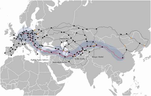
Table 12. Results of different KPIs in Scenario 4, Case I

Trains per day	Khorgos–Altynkol				Serakhs–Sarakhs				Kapikule–Kapitan Andreevo				Journey time
	Ql		Qt		Ql		Qt		Ql		Qt		Jt
	Avg	Max	Mean	Max	Avg	Max	Avg	Max	Avg	Max	Avg	Max	Avg	Max
20	0	1	0	0.1	29.71	81	3.27	8	94	37.69	7.73	16	21.4	34.3
40	77.23	180	4.05	9.6	80.8	180	8.08	17.6	83.82	186	15.51	30.4	38	67.9
60	174.66	380	9.02	19.2	126.08	270	12.19	25.6	129.47	276	23.09	48	54.7	99.9
80	273.45	580	14.01	28.8	171.4	360	16.28	35.2	174	368	30.67	64	71.3	138.3
100	375.45	780	19.15	41.6	216.749	450	20.37	41.6	219.81	460	38.25	76.8	88.1	176.7

Table 13. Results of different KPIs in Scenario 4, Case II

Trains per day	Khorgos–Altynkol				Turkmenbashi Seaport				Baku Seaport				Kapikule–Kapitan Andreevo				Journey time
	Ql		Qt		Ql		Qt		Ql		Qt		Ql		Qt		Jt
	Avg	Max	Avg	Max	Avg	Max	Avg	Max	Avg	Max	Avg	Max	Avg	Max	Avg	Max	Avg	Max
20	0	1	0	0.1	42.55	98	2.72	6.4	42.92	98	8.09	17.6	1.57	6	0.32	0.5	21.19	34
40	77.23	180	4.05	9.6	73.27	172	9.96	14.4	92.59	198	16.43	35.2	0	6	0.16	0.5	37.68	67.6
60	174.66	380	9.02	19.2	114.59	252	10.31	20.8	142.91	300	24.77	44.8	0	6	0	0.1	54.18	99.6
80	273.45	580	14.01	28.8	153.85	332	13.65	28.8	153.85	398	33.1	70.4	0	6	0	0.1	70.84	138
100	375.45	780	19.15	41.6	193.07	412	16.99	35.2	242.33	498	41.44	83.2	0	6	0	0.1	87.64	176.4

Table 14. Results of different KPIs in Scenario 5 (“-” is defined as not complied)

Trains per day	Alashankou-Dostyk				Khorgos-Altynkol				Erenhot-Zamiin Udd				Suifenhe-Pogranichny				Manzhouli-Zabaikal´sk				Serakhs-Sarakhs
	Ql		Qt		Ql		Qt		Ql		Qt		Ql		Qt		Ql		Qt		Qt		Qt
	Avg	Max	Avg	Max	Avg	Max	Avg	Max	Avg	Max	Avg	Max	Avg	Max	Avg	Max	Avg	Max	Avg	Max	Avg	Max	Avg	Max
	20	-	-	-	-	-	-	-	-	-	-	-	-	-	-	-	-	-	-	-	-	-	-	-
40	-	-	-	-	-	-	-	-	-	-	-	-	-	-	-	-	-	-	-	-	-	-	-	-
60	-	-	-	-	-	-	-	-	-	-	-	-	-	-	-	-	-	-	-	-	-	-	-	-
80	7.08	16.00	0.67	1.70	22.21	65.00	1.23	3.20	15.58	51.00	1.17	3.80	0.00	1.00	0.00	0.10	0.01	1.00	0.00	0.10	0.43	13.00	0.06	1.00
100	8.19	17.00	0.79	1.80	64.70	168.00	3.59	9.60	45.02	103.00	3.27	7.60	0.00	1.00	0.00	0.10	0.30	7.00	0.03	0.40	0.77	15.00	0.10	1.00
120	9.46	17.00	0.89	1.90	111.10	262.00	6.06	13.60	71.73	155.00	5.37	12.00	0.00	1.00	0.00	0.10	0.59	9.00	0.05	0.70	3.36	14.00	0.37	2.00
140	10.11	19.00	0.96	1.90	163.11	361.00	8.49	19.20	96.00	208.00	7.32	16.00	0.00	1.00	0.00	0.10	11.59	44.00	0.95	3.20	0.50	14.00	0.06	1.00
160	10.40	20.00	0.96	1.90	209.85	465.00	11.03	24.00	115.71	242.00	8.81	19.20	0.00	1.00	0.00	0.10	11.77	35.00	0.94	2.80	0.50	16.00	0.06	1.00

Table

Kapikule-Kapitan Andreevo				Brest-Malaszewicze				Kaliningrad				Case I		Case II
												Journey Time		Journey Time
Ql		Qt		Ql		Qt		Ql		Qt		Jt		Jt
Avg	Max	Avg	Max	Avg	Max	Avg	Max	Avg	Max	Avg	Max	Avg	Max	Avg	Max
-	-	-	-	-	-	-	-	-	-	-	-	9.30	13.10	9.43	13.10
-	-	-	-	-	-	-	-	-	-	-	-	9.48	14.30	9.82	13.10
-	-	-	-	-	-	-	-	-	-	-	-	10.62	16.70	11.31	16.70
17.32	50.00	3.92	8.80	5.75	31.00	0.60	2.60	47.23	157.00	2.72	6.40	12.74	22.30	13.86	23.90
27.69	74.00	5.78	12.80	5.49	30.00	0.55	2.40	66.93	200.00	3.60	8.80	15.09	31.90	16.54	31.90
49.81	118.00	9.65	20.80	6.42	31.00	0.59	2.60	72.90	207.00	3.92	8.80	17.75	43.10	18.77	35.10
51.38	117.00	9.91	20.80	6.09	34.00	0.53	2.60	98.03	273.00	5.04	11.20	19.88	49.50	21.42	43.10
57.26	129.00	10.83	22.40	4.95	30.00	0.43	2.40	124.55	331.00	6.22	14.40	22.14	55.90	23.85	46.30

Table 15. Comparison of three indexes—EMLI, GCI, and LPI

Emerging Market Logistics Index (EMLI)	Global Competitive Index (GCI)	Logistics Performance Index (LPI)
Issuing authority
Agility	World Economic Forum	World Bank Group
Countries
50	141	167
Components
“Domestic Logistics Opportunities” “International Logistics Opportunities” “Business Fundamentals”	“Institutions” “Infrastructure” “ICT adoption” “Macroeconomic stability” “Health” “Skills” “Product market” “Labor market” “Financial system” “Market size” “Business dynamism” “Innovation capability”	“Customs” “Infrastructure” “International shipments” “Logistics competence” “Tracking and tracing” “Timeliness”
Publication Years
2011–2020	2008–2019	2012, 2014, 2016, and 2018
Scale of measurement
0–10 (higher is better)	0–100 (higher is better)	1–5 (higher is better)
Methodology
Survey based. Equal aggregate of three components—33%. The three components are further divided into 16 indicators at disaggregate level holding same weightage for its component.	Survey based. There are 104 indicators at disaggregate level forming 12 components. An average to combine different indicators within each component followed by weight-based aggregation for 12 indicators. The results are then combined into a value by mean.	Survey based. Calculated by principal component analysis (PCA) to reduce data set dimensions. Values are normalized before doing PCA. LPI is very close the average of its components.
Literature review
Anatoliivna et al., 2016 use LPI and EMLI to study enterprise distribution system in the context of Ukraine but lacks a comparison between both.	Xia et al., 2012 highlight it to be lesser stable and concluded that GCI’s national culture indicator should be redefining by WEF for it to have better correlation with economy. (Raimbekov, et al., 2017 compare logistical weightage in different indicators in the context of EAEU countries, thus ranking them as follow (low-to-high): WCR by IMD (least logistics weightage) GGI by WEF DBI by WBG ETI by WEF LPI by WBG (most logistics weightage) Civelek et al., 2015 compare the effect of GDP and GCI and LPI as a mediator variable. Authors found it to be statistically significant.	Martí et al., 2014 relate LPI with international trade through gravity equations by region from 2007 to 2012. Rezaei et al., 2018 use Best Worst Method (BWM) to assign weightage to each of six indicators in contrast to equal weights. Beysenbaev & Dus, 2020 proposed an Improved LPI (ILPI), thus showing its effect on countries ranking due to its subjective nature. Luttermann et al., 2020 used empirical approach to compare GCI and LPI in 20 Asian countries through empirical methods with FDI and general trade and found LPI to be better than GCI for comparison.
Comments
Emerging markets only Socioeconomic inclination Lack of research articles	Inclined toward economic growth. Aggregate of indicators that are not important in this study in this study, thus lesser logistics weightage.	No inclination toward other parameters than logistics. Highest logistics weightage compared to other indexes.

References

- Abril, M., Barber, F., Ingolotti, L., Salido, M. A., Tormos, P., & Lova, A. (2008, September). An assessment of railway capacity. Transportation Research Part E: Logistics and Transportation Review, 445(5), 774–34. https://doi.org/https://doi.org/10.1016/j.tre.2007.04.001
- Anatoliivna, B. O., Fedorivna, G. O., & Oleksiivna, S. L. (2016). Development of the enterprise distribution system taking into account the regional logistics potential. Marketing and Management of Innovations, 2, 73–79.
- Arisha, A., & El Baradie, M. E. (2002, August 28–30). On the selection of simulation software for manufacturing application [Paper presentation]. Nineteenth International Manufacturing Conference (IMC-19),Queen’s University Belfast, N.Ireland
- Bababeika, M., Khademib, N., Chend, A., & Nasiri, M. (2017). Vulnerability analysis of railway networks in case of multi-link blockage. Transportation Research Procedia, 22, 275–284. https://doi.org/https://doi.org/10.1016/j.trpro.2017.03.034
- Baniya, S., Rocha, N., & Ruta, M. (2019). Trade effects of the new silk road. Policy Research Working Paper 8694. World Bank Group - Macroeconomics, Trade and Investment Global Practice. https://documents1.worldbank.org/curated/en/623141547127268639/pdf/Trade-Effects-of-the-New-Silk-Road-A-Gravity-Analysis.pdf
- Benjamin, P., Erraguntla, M., Delen, D., & Mayer, R. (1998). Simulation modeling at multiple levels of abstraction. s.l.: IEEE.
- Berger, R. (2017). STUDY - Eurasian rail corridors: What opportunities for freight stakeholders? International Union of Railways (UIC).
- Besenfelder, C., Kaczmarek, S., & Uygun, Y. (2013). Process-based cooperation support for complementary outtasking in production networks of SME. International Journal of Integrated Supply Management, 8(1/2/3), 121. https://doi.org/https://doi.org/10.1504/IJISM.2013.055072
- Beysenbaev, R., & Dus, Y. (2020). Proposals for improving the logistics performance Index. Asian Journal of Shipping and Logistics, 36(1), 34–42. https://doi.org/https://doi.org/10.1016/j.ajsl.2019.10.001
- Blanchard, J.-M. F., & Flint, C. (2017). The geopolitics of China’s maritime silk road initiative. Geopolitics, 22(2), 223–245. https://doi.org/https://doi.org/10.1080/14650045.2017.1291503
- Burdett, R. L., & Kozan, E. (2006). Techniques for absolute capacity determination in railways. Transportation Research Part B: Methodological, 40(8), 616–632. https://doi.org/https://doi.org/10.1016/j.trb.2005.09.004
- CAREC. (2018). Corridor performance measurement and monitoring 2018. ADB.
- Cichenski, M.,Jaehn, F., Pawlak, G. Pesch, E., Singh, G., & Blazewicz, J. (2016). An integrated model for the transshipment yard scheduling problem. Journal of Scheduling, 20, 57–65. https://doi.org/https://doi.org/10.1007/s10951-016-0470-4
- Civelek, M. E., Uca, N., & Çemberci, M. (2015). The mediator effect of logistics performance index on the relation between global competitiveness index and gross domestic product. European Scientific Journal, 11(13). https://eujournal.org/index.php/esj/article/view/5658
- Cole, T. (2020). Soaring air freight rates add value to China-Europe rail [Interview] (8 April 2020). Journal of Commerce online
- DB AG. (2018). FESCO and DB Cargo Russija Сo.Ltd plan to start joint transit transports from China via Kaliningrad to Europe. https://ru.dbcargo.com/rail-russijaservices-en/News_Media/news/FESCO-and-DB-Cargo-3399362
- Dessouky, M. M., & Leachman, R. C. (1995). A simulation modeling methodology for analyzing large complex rail networks. Simulation, 65(2), 131–142. https://doi.org/https://doi.org/10.1177/003754979506500205
- DHL. (2019). DHL LAUNCHES FASTEST RAIL FREIGHT SERVICE BETWEEN CHINA AND GERMANY. DHL. Retrieved April 13, 2020, from https://www.dhl.com/cn-en/home/press/press-archive/2019/dhl-launches-fastest-rail-freight-service-between-china-and-germany.html
- Dimitrov, S. D. (2011). Simplified border checkpoint simulation model. http://mech-ing.com/journal/Archive/2011/3/91.dimitrov.tm11.pdf
- DSV. (2019). Rail freight transport between China and Europe.DSV Global Transport and Logistics. https://www.dsv.com/en/insights/expert-opinions/rail-freight-between-europe-and-china
- Dubey, R., Gunasekaran, A., & Singh, S., & Sushil. (2015). Building theory of sustainable manufacturing using total interpretive structural modelling. International Journal of Systems Science: Operations & Logistics, 2(4), 231–247. https://doi.org/https://doi.org/10.1080/23302674.2015.1025890
- ESCAP. (2018). Study on border crossing practices in international railway transport. United Nations.
- Feng, F., Zhang, T., Liu, C., & Fan, L. (2020). China Railway Express Subsidy Model Based on Game Theory under “the Belt and Road” Initiative. Sustainability, 12(5), 2083. https://doi.org/https://doi.org/10.3390/su12052083 https://doi.org/https://doi.org/10.3390/su12052083
- Freund, C., & Ruta, M., (2018). Belt and road initiative. World Bank Group. https://www.worldbank.org/en/topic/regional-integration/brief/belt-and-road-initiative
- Güller, M., Karakaya, E., Uygun, Y., & Hegmanns, T. (2018). Simulation-based performance evaluation of the cellular transport system. Journal of Simulation, 12(3), 225–237. https://doi.org/https://doi.org/10.1057/s41273-017-0061-1
- Güller, M., Uygun, Y., & Karakaya, E. (2013). Multi-agent simulation for concept of cellular transport system in intralogistics. In A. Azevedo (Ed.), Advances in sustainable and competitive manufacturing systems - Lecture notes in mechanical engineering (pp. 233–244). Springer.
- Güller, M., Uygun, Y., & Noche, B. (2015). Simulation-based optimization for a capacitated multi-echelon production-inventory system. Journal of Simulation, Volume , 9(4), 325–336. https://doi.org/https://doi.org/10.1057/jos.2015.5
- Haiquan, L. (2017). The security challenges of the “One Belt, One Road” initiative and China’s choices. CIRR, 23(78), 129–147. https://doi.org/https://doi.org/10.1515/cirr-2017-0010
- He, H. (2016). Key Challenges and Countermeasures with Railway Accessibility along the Silk Road. Engineering, 2(13), 288–291. 20 September. https://doi.org/https://doi.org/10.1016/J.ENG.2016.03.017
- Heshmati, S., Kokkinogenis, Z., & Rossetti, R. J. F. A. M. (2016). An agent-based approach to schedule crane operations in rail-rail transshipment terminals. Computational Management Science - Lecture Notes in Economics and Mathematical Systems, 682, 91–97. https://doi.org/https://doi.org/10.1007/978-3-319-20430-7_12
- Hillman, J. E. (2018). The rise of China-Europe railways. Center for Strategic and International Studies. www.csis.org/analysis/rise-china-europe-railways
- Huang, H., Li, K., & Wang, Y. (2018). A simulation method for analyzing and evaluating rail system performance based on speed profile. Journal of Systems Science and Systems Engineering, 27(6), 810–834. https://doi.org/https://doi.org/10.1007/s11518-017-5358-0
- IRU. (2017). New Eurasian Land Transport Initiative (NELTI). IRU. https://www.iru.org/where-we-work/iru-in-eurasia-and-russia/new-eurasian-land-transport-initiative-nelti
- Isik, M. Cekyay, B., Ülengin, F., Kabak, Ö., Ekici, Ö., Özaydin, S., Toktas Palut, P., Bozkaya, B.,Topcu, Y. I. (2017). Logistics process improvement of Kapikule border crossing. The 15th International Logistics and Supply Chain Congress (LMSCM) (pp. 1–11), Dogus University,Istanbul, Turkey. https://hdl.handle.net/11376/3244
- Islam, D., Zunder, T., Jackson, R., Nesterova, N., & Burgess, A. (2013). The potential of alternative rail freight transport corridors between central europe and china. Transport Problems, 8(4), 45–57. https://www.researchgate.net/publication/289798617_The_potential_of_alternative_rail_freight_transport_corridors_between_central_europe_and_china
- Jakóbowski, J., Popławski, K., & Kaczmarski, M. (2018). The Silk Railroad. The EU-China rail connections: Background, actors, interests. Ośrodek Studiów Wschodnich (OSW).
- Koch, M., & Tolujew, J. (2013). Grouping logistics objects for mesoscopic modeling and simulation of logistics systems. Aalesund, s.n.
- Kortmann, C., & Uygun, Y. (2007). Organizational flow design of the implementation of integral production systems [Ablauforganisatorische Gestaltung der Implementierung von Ganzheitlichen Produktionssystemen]. ZWF Zeitschrift fuer Wirtschaftlichen Fabrikbetrieb, 102(10), 635–639. https://doi.org/https://doi.org/10.3139/104.101195
- Kosoy, V. (2018). A future of EU-EAEU-China cooperation in trade and railway transport,” Infrastructure economics centre. sl.: UNECE.
- Landex, A. (2008). Methods to estimate railway capacity and passenger delays. Technical University of Denmark.
- Leijen, M. v. (2019). New silk road milestone: more traffic eastbound to chongqing in 2018. RailFreight.com. https://www.railfreight.com/specials/2019/01/08/europe-bound-traffic-from-chongqing-china-booms-in–2018
- Lindfeldt, A. (2015). Railway capacity analysis: Methods for simulation and evaluation of timetables, delays and infrastructure. KTH Royal Institute of Technology.
- Lu, Q., Dessouky, M., & Leachman, R. C. (2004). Modeling train movements through complex rail networks. ACM Transactions on Modeling and Computer Simulation, 14(1), 48–75. https://doi.org/https://doi.org/10.1145/974734.974737
- Luttermann, S., Kotzab, H., & Halaszovich, T. (2020). The impact of logistics performance on trade. World Review of Intermodal Transportation Research (WRITR), 9(1), 27–46. https://doi.org/https://doi.org/10.1504/WRITR.2020.106444
- Lyutov, A., Uygun, Y., & Hütt, M.-T. (2019). Managing workflow of customer requirements using machine learning. Computers in Industry, 109, 215–225. https://doi.org/https://doi.org/10.1016/j.compind.2019.04.010
- Lyutov, A., Uygun, Y., & Hütt, M.-T. (2021). Machine learning misclassification of academic publications reveals non-trivial interdependencies of scientific disciplines. Scientometrics, 126(2), 1173–1186. https://doi.org/https://doi.org/10.1007/s11192-020-03789-8
- Marinov, M., Sahin, I., Ricci, S., & Vasic-Franklin, G. (2013). Railway operations, time-tabling and control. Research in Transportation Economics, 41(1), 59–75. https://doi.org/https://doi.org/10.1016/j.retrec.2012.10.003
- Martí, L., Puertas, R., & García, L. (2014). The importance of the logistics performance index in international trade. Applied Economics, 46(22), 982–2992. https://doi.org/https://doi.org/10.1080/00036846.2014.916394
- Mattsson, L.-G. (2007). Railway capacity and train delay relationships. In A. T. Murray & T. H. Grubesic (Eds.), Critical Infrastructure: Reliability and Vulnerability (pp. 129–150). Springer.
- MERICS. (2018). Mercator Institute for China Studies (MERICS). [Online] Retrieved June 11, 2020, from https://merics.org/en/analysis/mapping-belt-and-road-initiative-where-we-stand
- NIIAT. (2017). Draft report of the phase III of the Euro-Asian Transport Links project. Economic Commission for Europe.
- Özgür, A., Uygun, Y., & Hütt, M.-T. (2021). A review of planning and scheduling methods for hot rolling mills in steel production. Computers and Industrial Engineering, 151, 106606. https://doi.org/https://doi.org/10.1016/j.cie.2020.106606
- Portal, B. R. I., 2019. The six years of the “Belt and Road”-Facilities Connect. Belt and Road Portal. https://www.yidaiyilu.gov.cn/ydylcylznzd/cjc/102467.htm
- Pouryousef, H., Lautala, P., & White, T. (2015). Railroad capacity tools and methodologies in the U.S. and Europe. Journal of Modern Transportation, 23(1), 30–42. https://doi.org/https://doi.org/10.1007/s40534-015-0069-z
- Raimbekov, Z. S., Syzdykbayeva, B. U., Mussina, K. P., Moldashbayeva, L. P., & Zhumataeva, B. A. (2017). The study of the logistics development effectiveness in the Eurasian Economic Union countries and measures to improve it. European Research Studies Journal, 20(4), 260–276. https://doi.org/https://doi.org/10.35808/ersj/889
- Reed, T., & Trubetskoy, A. (2019). Assessing the value of market access from belt and road projects. sl.: The World Bank Group.
- Reynolds, E., & Uygun, Y. (2018). Strengthening advanced manufacturing innovation ecosystems: The case of Massachusetts. Technological Forecasting and Social Change, 136, 178–191. https://doi.org/https://doi.org/10.1016/j.techfore.2017.06.003
- Rezaei, J., Roekel, W. V., & Tavasszy, L. (2018). Measuring the relative importance of the logistics performance index indicators using Best Worst Method. Transport Policy, 68, 158–169. https://doi.org/https://doi.org/10.1016/j.tranpol.2018.05.007
- Ruta, M. de Soyres, F., Mulabdic, A., Murray, S., & Rocha, N. 2018. How much will the Belt and Road Initiative reduce trade costs? Policy Research Working PaperNo. 8614. Washington, DC.:World Bank Group. https://openknowledge.worldbank.org/handle/10986/30582
- Sameni, M. K., Dingler, M., Preston, J. M., & Barkan, C. P. (2011). Profit-Generating capacity for a freight railroad. Technical University of Denmark, DTU.
- Sayyadi, R., & Awasthi, A. (2018). A simulation-based optimisation approach for identifying key determinants for sustainable transportation planning. International Journal of Systems Science: Operations & Logistics, 5(2), 161–174. https://doi.org/https://doi.org/10.1080/23302674.2
- Sayyadi, R., & Awasthi, A. (2020). An integrated approach based on system dynamics and ANP for evaluating sustainable transportation policies. International Journal of Systems Science: Operations & Logistics, 7(2), 182–191. https://doi.org/https://doi.org/10.1080/23302674.2018.155
- Straub, N., Schmidt, A., & Uygun, Y. (2013). e-Qualification for efficient logistics processes [e-Qualifizierung für effiziente Logistikprozesse: Anforderungen an die Gestaltung von betrieblichen Weiterbildungsprozessen]. ZWF Zeitschrift fuer Wirtschaftlichen Fabrikbetrieb, 108(6), 405–409. https://doi.org/https://doi.org/10.3139/104.110958
- TCITR. 2020. ROUTE. Middle Corridor. Retrieved June 10, 2020, from https://middlecorridor.com/en/route
- Thürer, M., Tomašević, I., Stevenson, M., Blome, C., Melnyk, S., Chan, H. K., & Huang, G. Q. (2020). A systematic review of China’s belt and road initiative: Implications for global supply chain management. International Journal of Production Research, 58(8), 2436–2453. https://doi.org/https://doi.org/10.1080/00207543.2019.1605225
- UNECE. (2015). Information from participants on recent developments in transport infrastructure priority projects on EATL routes. EC.
- Uygun, Y., Hasselmann, V.-R., & Piastowski, H. (2011). Diagnosis and optimization of the production based on the overall production system in its entirety [Diagnose und Optimierung der Produktion auf Basis Ganzheitlicher Produktionssysteme]. ZWF Zeitschrift fuer Wirtschaftlichen Fabrikbetrieb, 106(1/2), 55–58. https://doi.org/https://doi.org/10.3139/104.110503
- Uygun, Y., & Jafri, S. A. I. (2020). Controlling risks in sea transportation of cocoa beans. Cogent Business and Management, 7(1). https://doi.org/https://doi.org/10.1080/23311975.2020.1778894
- Uygun, Y., & Straub, N. (2013). Supply chain integration by human-centred alignment of lean production systems. In H-J. Kreowski, B. Scholz-Reiter, & K-D. Thoben (Eds.), Lecture notes in logistics (pp. 93–112). Springer.
- Velde, D. V. D. (1999). Organisational forms and entrepreneurship in public transport: Classifying organisational forms. Transport Policy, 6(3), 147–157. https://doi.org/https://doi.org/10.1016/S0967-070X(99)00016-5
- Wagner, N., Aritua, B., & Zhu, T. (2019). The New Silk Road: Opportunities for Global Supply Chains and Challenges for Further Development. [Online]. https://wagener-herbst.com/wp-content/uploads/sites/10/2020/04/20191118_WSL-Forum_NewSilkRoad_Presentation.pdf
- WBG. 2018. World bank group. World Bank Group. Retrieved June 1, 2020, from https://lpi.worldbank.org/international
- Woroniuk, C., & Marinov, M. (2013). Simulation modelling to analyse the current level of utilisation of sections along a rail route. Journal of Transport Literature, 7(2), 235–252. https://doi.org/https://doi.org/10.1590/S2238-10312013000200012
- Xia, R., Liang, T., Zhang, Y., & Wu, S. (2012). Is global competitive index a good standard to measure economic growth? A suggestion for improvement. International Journal of Services and Standards, 8(1), 45–57. https://doi.org/https://doi.org/10.1504/IJSS.2012.048438
- Xu, J., & Herrero, A. G. (2017). China’s belt and road initiative: can europe expect trade gains? China and World Economy, 25(6), 84–99. https://doi.org/https://doi.org/10.1111/cwe.12222
- Yan, Z., & Filimonov, V. (2018). COMPARATIVE STUDY OF INTERNATIONAL CARRIAGE OF GOODS BY RAILWAY BETWEEN CIM AND SMGS. Frontiers of Law in China, 13 (1), 115–136. https://doi.org/https://doi.org/10.3868/s050-007-018-0008-5
- Zhang, X., & Schramm, H.-J. (2018, June 13). Eurasian rail freight in the one belt one road era. 30th Annual NOFOMA Conference: Relevant Logistics and Supply Chain Management Research, University of Southern Denmark, Kolding, Denmark.