Non-performing loans and the lending channel of shock transmission across countries

Abstract

Recent international macroeconomics literature on global imbalances explains the U.S. persistent current account deficit and emerging countries’ surplus. Little research has been done at the banking-sector level, where U.S. banks are lenders to banks in emerging countries. We build a two-country framework where banks are explicitly modeled to investigate how lending in the banking sector can affect the international macroeconomy during the financial crisis of 2007–2008. In the steady state, banks in the developing country borrow from the U.S. banks. When the borrowers in the U.S. pay back less than contractually agreed and damage the balance sheet of the U.S. banks, with the presence of bank capital requirement constraint, U.S. banks raise lending rates and decrease the loans made to U.S. borrowers as well as banks in the developing country. The results are a sharp increase in the lending spread, a reduction in output and a depreciation in the real exchange rate of the developing country. This is the experience of many emerging Asian markets following the U.S. financial crisis starting in late 2007. Another feature of our model captures an empirical fact, documented by Devereux and Yetman, that across different economies, countries with lower financial ratings can suffer more when the lending country deleverages.

Keywords:

• International finance
• financial crisis
• bank deleverage
• real exchange rate
• emerging Asian markets

PUBLIC INTEREST STATEMENT

The paper highlights the importance of bank lending channel in transmitting shocks across countries. When U.S banks suffer losses, they contract their balance sheet and start calling off loans, including those made to developing countries. The results are a sharp increase in the lending spread, a reduction in output and a depreciation in the real exchange rate of the developing country. This is the experience of many emerging Asian markets following the U.S. financial crisis starting in late 2007. Countries with lower financial ratings also suffer more, as documented by Devereux and Yetman (2010).

1. Introduction

International macroeconomics literature on global imbalances explains why the U.S. runs a persistent current account deficit. The U.S. is the net borrower at the country level.¹ At the banking-sector level, this is not necessarily the case. U.S. banks and banks in other developed economies are net lenders to banks in emerging Asian markets (EAM). Starting from April, 2007, losses in the mortgage market began to damage U.S. banks’ balance sheets (Figures 1 and 2), U.S. banks deleveraged and reduced deposits and credits (Figure 3). Not only did they contract loans made to U.S. borrowers, they contracted loans made to foreign borrowing banks as well. Figure 4 documents external (cross-border) assets of banks in developed economies and Figure 5 documents external liabilities of banks in EAM. With the exception of Japan, which was little exposed to U.S. Mortgage Backed Securities (MBS), all major developed economies showed significant contractions in banks’ external assets, which resulted in significant contractions in EAM banks’ external liabilities.² The documented contraction in international inter-bank lending was followed by a worldwide drop in GDP growth, both among the developed world (Figure 6) and the developing world (Figure 7). This empirical evidence highlights the importance of the banking system in international transmission of shocks.

Figure 1. New delinquent balances by loan type.Source: Federal Reserve Bank of New York (2013)

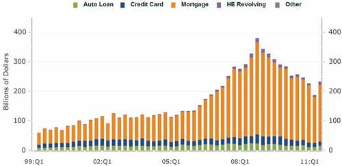
Figure 2. Percent of mortgage debt 90+ days late by state (U.S. data).Source: Federal Reserve Bank of New York (2013)

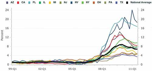
Figure 3. U.S bank assets and liabilities.Source: Board Governors of Federal Reserve System (2012)

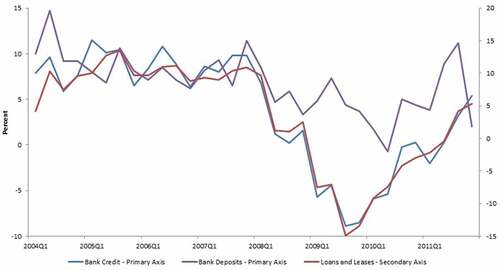
Figure 4. External assets of banks in developed economies.Source: Bank for International Settlement (2012)

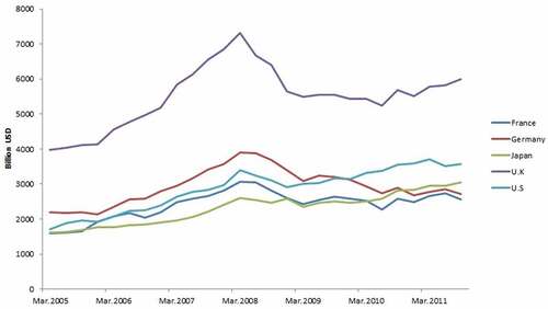
Figure 5. External liabilities of banks in emerging Asian markets.Source: Bank for International Settlement (2012)

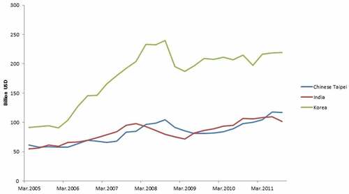
Figure 6. GDP growth of developed economies.Source: World Bank (2012)

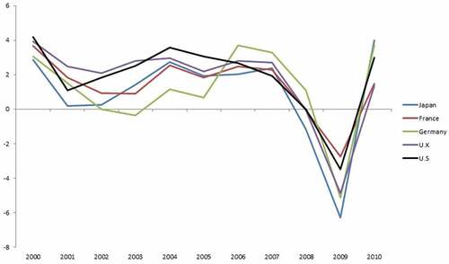
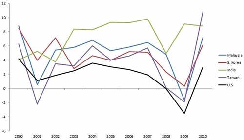
Figure 7. GDP growth of the U.S. and developing economies.Source: World Bank (2012)

The financial crisis of 2007–2008 in the U.S. was characterized by decline in asset prices, disruption in the loan market, sharp increase in interest rate spread and a large drop in GDP. One thing many scholars have agreed is that the banking system played a vital role in this crisis. There are a number of recent working papers that include bank in a closed economy dynamic stochastic general equilibrium (DSGE) model to model the recent crisis in the U.S. (Gertler and Kiyotaki (2010), Iacoviello and Neri (), and a series of papers by Dib (2010a and 2010b)). Recent development in international macroeconomics literature investigates the effect of the financial linkage that spread the U.S. mortgage crisis worldwide. Devereux and Yetman (2010) and van Wincoop (2011) build international portfolio models where leveraged investors in one country hold the financial asset in the other country. Consequently, any shock that affects the domestic country asset prices will affect foreign investors’ balance sheets and spread to the foreign economy. Ueda (2010), Kollmann et al. (2011) and Kalemli-Ozcan, Papaioannou and Perri (2011) build international business cycle models with banks. In these papers, entrepreneurs in two countries share a common lender(s). Any shock that hits one economy will affect the common lender(s) and thus, its (their) borrowers. While both of these features can be true in the developed world, i.e., U.S. and the Euro Area, they are not the best to describe the recent crisis for the EAM. Contrary to the large portfolio position of European banks in U.S. MBS, banks in EAM have no or very little exposure to the U.S. MBS and firms in these countries have little direct access to foreign bank credits.

This study builds a two-country model with the banking system that plays an important role in international transmission of shock, which has been largely agreed to be the main cause of the recent crisis. Our model is built upon the closed-economy version in Iacoviello and Neri (). In steady state, banks in the developing country (EAM/domestic country) borrow from banks in the developed country (the U.S./foreign country). When some borrowers in the U.S. pay back less than contractually agreed, with the presence of capital requirement constraint, U.S. banks cut back on lending to U.S. borrowers as well as EAM banks and raise the interbank lending rate. Domestic banks now face more expensive and less available foreign credit, and will reduce loans made to domestic borrowers. The financial (repayment) shock in the U.S. Is transmitted across country via the banking system.

In another exercise, we investigate the behavior of the model under permanent and temporary shocks to the weight of domestic bank loan in the foreign bank’s capital requirement constraint. The permanent shock can be interpreted as a change in bank regulation, such as moving from Basel I to Basel II. A temporary shock can be interpreted as an exogenous drop in domestic banks’ credit ratings. The results for these shocks are reductions in home output, investment and consumption and a depreciation of home real exchange rate.

Our paper is related to a number of empirical papers on global banking. Peek and Rosengren (1997) studied the behavior of Japanese banks in the U.S. During the financial crisis in the late 1980s and early 1990s in Japan, Japanese banks in the U.S. substantially contracted the amount of loans made to U.S. borrowers. Cetorelli and Goldberg (2012) document that “foreign lending activity of U.S. bank affiliates abroad can rely less on the overall strength of the home office in times of tighter monetary condition in the U.S.”. Popov and Udell (2010) found that financial distress by West European and U.S. parent banks has a significant impact on the availability of business loans for East European firms. Most recently, Imai and Takarabe (2011) used the data from nationwide and local banks in Japan to test whether banking integration plays an important role in transmitting financial shocks across geographical boundaries. They found that nation-wide banks do indeed transmit financial shocks originated from major cities to smaller local economies. The results of our model under different weights of interbank loan in the capital requirement constraint suggests that across countries, lower-rated economies will suffer more when U.S. banks deleverage. This is consistent with empirical evidence for the recent crisis, documented by Devereux and Yetman (2010).

2. The model

There are two countries: the domestic country (EAM) and the foreign country (U.S.).³ In each country, there are five types of agents: patient households, impatient households, entrepreneurs, firms and banks. There are two sectors in the economy: the tradable and non-tradable goods sectors.

Both patient and impatient households (HHs) work for firms in tradable and non-tradable sectors. They earn wage income and consume tradable goods, non–tradable goods and housing. Patient HHs supply deposits for banks and earn a return from the deposits. Impatient HHs, on the other hand, borrow from banks to consume. They can only borrow up to a fraction of the value of their collateral (house).

Domestic bankers take the deposit from domestic depositors and can also borrow in the international interbank market. They can only borrow up to a fraction of the value of their capital. They pay a return for the fund they borrow and lend it to domestic borrowers for a higher return. Foreign bankers take the deposit from foreign depositors. They lend out to foreign borrowers and domestic bankers. Domestic and foreign bankers face capital requirement constraint.

Entrepreneurs accumulate physical capital used in both tradable and nontradable sectors. They finance their investment with income from capital rental and bank loan, which is subject to a collateral debt constraint.

Firms in the tradable and nontradable sectors use capital and labor to produce goods. They pay wages to HHs.

2.1. Consumption basket

Consumers’ consumption aggregate is given by: $c_t={\left[{\left(c_t^N\right)}^{\frac{\omega -1}{\omega }}+{\left(c_t^T\right)}^{\frac{\omega -1}{\omega }}\right]}^{\frac{\omega }{\omega -1}}$, where $c_t^T$ and $c_t^N$ are tradable and non-tradable consumptions. The corresponding price index is $P_t={\left[{\left(P_t^N\right)}^{1-\omega }+{\left(P_t^T\right)}^{1-\omega }\right]}^{\frac{1}{1-\omega }}$ where $P^N$ and $P^T$ are the tradable and non-tradable price indices. The consumption aggregate and price indices for the foreign economy are identical. We denote the price of tradable (non-tradable) relative to the price of consumption baskets as $p_t^T$ and $p_t^N$.

2.2. Patient HHs

A continuum of domestic patient HHs deposit ${\mathrm{d}}_t$, consume composite good $c_{p,t}$ and housing $h_{p,t}$, and supply labor to tradable and non-tradable sectors ($n_{p,t}^T$ and $n_{p,t}^N$ respectively). They earn wage income and return from their deposits. They maximize the infinite sum of utilities:

$\underset{c_{p,t},h_{p,t},n_{p,t}^T,n_{p,t}^N,{\mathrm{d}}_t}{max}{E}_0\sum _{t=0}^{\mathrm{\infty }}{\beta }_p^t\left[\ln c_{p,t}+v\ln h_{p,t}+{\tau }_p\ln \left(1-n_{p,t}^T-n_{p,t}^N\right)\right],$

subject to the budget constraint:

(1) $c_{p,t}+{\mathrm{d}}_t+q_t\mathrm{\Delta }{h}_{p,t}=R_{d,t}{\mathrm{d}}_{t-1}+w_{p,t}^N{n}_{p,t}^N+w_{p,t}^T{n}_{p,t}^T$(1)

where $R_{d,t}$ is the return from the deposits and $q_t$ is the price of a house. $w_{p,t}^T$ and $w_{p,t}^N$ are wages from the tradable and non-tradable sectors, respectively. Their first-order conditions are:

(2) $\frac{1}{c_{p,t}}={\beta }_p{E}_t\left(\frac{R_{d,t+1}}{c_{p,t+1}}\right)$(2)

(3) $\frac{q_t}{c_{p,t}}=\frac{v}{h_{p,t}}+{\beta }_p{E}_t\left(\frac{q_{t+1}}{c_{p,t+1}}\right)$(3)

(4) $\frac{w_{p,t}^N}{c_{p,t}}=\frac{{\tau }_p}{1-n_{p,t}^T-n_{p,t}^N}$(4)

(5) $\frac{w_{p,t}^T}{c_{p,t}}=\frac{{\tau }_p}{1-n_{p,t}^T-n_{p,t}^N}$(5)

Foreign patient HHs’ optimization problem are identical and indexed with *.

2.3. Impatient HHs

Domestic impatient HHs also consume goods and housing, and supply labor. $c_{i,t},h_{i,t},n_{i,t}^T,n_{i,t}^N$ are impatient HHs’ consumptions, houses, labor supply to the tradable and non-tradable sectors. Unlike patient HHs, they borrow money from banks, $l_{i,t}$, to finance consumption. They pay interest $R_{i,t}$ on the loan and can only borrow up to the value of their houses. Their maximization problem is:

$\underset{c_{i,t},h_{i,t},n_{i,t}^T,n_{i,t}^N,l_{i,t}}{max}{E}_0\sum _{t=0}^{\mathrm{\infty }}{\beta }_i^t\left[\mathit{\text{ln}}{c}_{i,t}+\mathit{\text{vln}}{h}_{i,t}+{\tau }_i\mathit{\text{ln}}\left(1-n_{i,t}^N-n_{i,t}^T\right)\right],$

subject to the budget constraint:

(6) $c_{i,t}+q_t\mathrm{\Delta }{h}_{i,t}+R_{i,t}{l}_{i,t-1}=l_{i,t}+w_{i,t}^N{n}_{i,t}^N+w_{i,t}^T{n}_{i,t}^T$(6)

and the borrowing constraint following Kiyotaki and Moore (1997):

(7) $l_{i,t}\le m_i{E}_t\left(\frac{q_{t+1}{h}_{i,t}}{R_{i,t}}\right)$(7)

Foreign impatient HHs’ problem is equivalent, except that in their budget constraint, there is a repayment shock. Their budget constraint is:

$c_{i,t}^{\ast }+q_t^{\ast }\mathrm{\Delta }{h}_{i,t}^{\ast }+R_{i,t}^{\ast }{l}_{i,t-1}^{\ast }-{\in }_t=l_{i,t}^{\ast }+w_{i,t}^{N\ast }{n}_{i,t}^{N\ast }+w_{i,t}^{T\ast }{n}_{i,t}^{T\ast }$

As in Iacoviello and Neri (), ${\in }_t$ is a mean zero, AR(1) shock that captures the exogenous repayment shock in the U.S. When ${\in }_t$ is greater than 0, U.S. impatient HHs pay back less than their debt obligation.

First-order conditions of impatient HHs are:

(8) $\frac{1}{c_{i,t}}={\lambda }_{i,t}{R}_{i,t}+{\beta }_i{E}_t\left(\frac{R_{i,t+1}}{c_{i,t+1}}\right)$(8)

(9) $\frac{q_t}{c_{i,t}}=\frac{v}{h_{i,t}}+{\lambda }_{i,t}{m}_i{E}_t\left(q_{t+1}\right)+{\beta }_i{E}_t\left(\frac{q_{t+1}}{c_{i,t+1}}\right)$(9)

(10) $\frac{w_{i,t}^N}{c_{i,t}}=\frac{{\tau }_i}{1-n_{i,t}^N-n_{i,t}^T}$(10)

(11) $\frac{w_{i,t}^T}{c_{i,t}}=\frac{{\tau }_i}{1-n_{i,t}^N-n_{i,t}^T}$(11)

${\lambda }_{i,t}$ is the Lagrangian multiplier of impatient HHs’ borrowing constraint.

2.4. Entrepreneurs

Entrepreneurs’ optimization problem is:

$\underset{c_{e,t}, k_t^N,k_t^T,l_{e,t}}{\mathit{\text{max}}}{E}_0\sum _{t=0}^{\mathrm{\infty }}{\beta }_{\mathrm{e}}^t\mathit{\text{ln}}{c}_{\mathrm{e},t},$

subject to the budget constraint:

$c_{e,t}+k_t^N+k_t^T+R_{e,t}{l}_{e,t-1}+\frac{{\varphi }_k}{2}{\left(\mathrm{\Delta }{k}_t^N\right)}^2+\frac{\varphi k}{2}{\left(\mathrm{\Delta }{k}_t^T\right)}^2$

(12) $=l_{e,t}+\left(r_{k,t}^N+1-\delta \right)k_{t-1}^N+\left(r_{k,t}^T+1-\delta \right)k_{t-1}^T$(12)

and the borrowing constraint:

(13) $l_{e,t}\le m_e\left(k_t^N+k_t^T\right)$(13)

where $c_{e,t}$ is entrepreneurs’ consumption. $k_t^N,k_t^T$ are entrepreneurs’ capital in the tradable and nontradable sectors. They finance investment with income from capital rental in the two sectors $r_{k,t}^N+1,r_{k,t}^T+1$ and bank loan $l_{e,t}$. The bank loan cannot exceed the value of their capital. Entrepreneurs pay banks a return $R_{e,t}$ on the loan. Similar to Backus et al. (1994), we assume that investment uses the same goods composite as the consumption basket. $\frac{{\varphi }_k}{2}{\left(\mathrm{\Delta }{k}_t^N\right)}^2,\frac{{\varphi }_k}{2}{\left(\mathrm{\Delta }{k}_t^T\right)}^2$ are convex capital adjustment costs that entrepreneurs face when they change their stock of capital in the tradable and non-tradable sectors. Entrepreneurs’ first order conditions are:

(14) $\frac{1}{c_{e,t}}\left(1+{\varphi }_k\mathrm{\Delta }{k}_t^N\right)=\frac{{{\lambda }_{e,t}}^{\prime }}{c_{e,t}}{m}_e+{\beta }_e{E}_t\left\{\frac{1}{c_{e,t+1}}\left[\left(r_{k,t+1}^N+1-\delta \right)+{\varphi }_k\mathrm{\Delta }{k}_{t+1}^N\right]\right\}$(14)

(15) $\frac{1}{c_{e,t}}\left(1+{\varphi }_k\mathrm{\Delta }{k}_t^T\right)=\frac{{{\lambda }_{e,t}}^{\prime }}{c_{e,t}}{m}_e+{\beta }_e{E}_t\left\{\frac{1}{c_{e,t+1}}\left[\left(r_{k,t+1}^T+1-\delta \right)+{\varphi }_k\mathrm{\Delta }{k}_{t+1}^T\right]\right\}$(15)

(16) $\frac{1}{c_{e,t}}=\frac{{{\lambda }_{e,t}}^{\prime }}{c_{e,t}}+{\beta }_e{E}_t\left(\frac{R_{e,t+1}}{c_{e,t+1}}\right)$(16)

where $\frac{{{\lambda }_{e,t}}^{\prime }}{c_{e,t}}$ is the Lagrangian multiplier of entrepreneurs’ borrowing constraint. Foreign entrepreneurs’ problems and first-order conditions are similar.

2.5. Bankers

Domestic Bankers: Domestic bankers borrow from domestic depositors and foreign banks and supply loans to impatient HHs and entrepreneurs. The funds they obtain from the foreign bank is in units of tradable goods. They pay returns on the funds they borrow, $R_{d,t}$ and $R_{f,t}$, to depositors and foreign banks, respectively. They charge higher interests on the loans they lend out: $R_{i,t}$ and $R_{e,t}$ to impatient HHs and entrepreneurs. They face a capital requirement constraint and a collateral debt constraint. The two constraints together pin down the level of foreign assets in the model. Their optimization problem is:

$\underset{c_{b,t},d_t,l_{i,t},l_{e,t},l_{f,t}}{max}{E}_0\sum _{t=0}^{\mathrm{\infty }}{\beta }_b^t\mathit{\text{ln}}{c}_{b,t},$

subject to the budget constraint:

(17) $c_{b,t}+R_{d,t}{d}_{t-1}+l_{e,t}+l_{i,t}+R_{f,t}{p}_t^T{l}_{f,t-1}=d_t+R_{e,t}{l}_{e,t-1}+R_{i,t}{l}_{i,t-1}+p_t^T{l}_{f,t}-\left\{\begin{array}{c}\frac{{\varphi }_e}{2}{\left(\mathrm{\Delta }{l}_{e,t}\right)}^2+\frac{{\varphi }_i}{2}{\left(\mathrm{\Delta }{l}_{i,t}\right)}^2+\\ \frac{{\varphi }_d}{2}{\left(\mathrm{\Delta }{d}_t\right)}^2+\frac{{\varphi }_f}{2}{\left(\mathrm{\Delta }{p}_t^T{l}_{f,t}\right)}^2\end{array}\right\}$(17)

the capital requirement constraint:

(18) $d_t+p_t^T{l}_{f,t}\le {\gamma }_e{l}_{e,t}+{\gamma }_i{l}_{i,t}$(18)

and the foreign debt constraint:

(19) $p_t^T{l}_{f,t}\le m_f\left(\frac{l_{i,t}+l_{e,t}-d_t}{R_{f,t}}\right)$(19)

The international inter-bank loan $l_{f,t}$ is denominated in tradable good price. In domestic consumption, its value is $p_t^T{l}_{f,t}$. Domestic bankers use their capital as collateral, which is equal to total assets $l_{e,t}+l_{i,t}$ minus liability $d_t$. Ali Dib (2010b) made a similar assumption on the interbank lending constraint. $m_f$ is the loan to value in the international financial market. $\frac{{\varphi }_e}{2}{\left(\mathrm{\Delta }{l}_{e,t}\right)}^2,\frac{{\varphi }_i}{2}{\left(\mathrm{\Delta }{l}_{i,t}\right)}^2,\frac{{\varphi }_d}{2}{\left(\mathrm{\Delta }{d}_t\right)}^2,\frac{{\varphi }_f}{2}{\left(\mathrm{\Delta }{p}_t^T{l}_{f,t}\right)}^2$ are adjustment costs that banks face when they change their loans and deposits. Their first order conditions are:

(20) $\frac{1}{c_{b,t}}\left[1-{\varphi }_d\mathrm{\Delta }{d}_t\right]=\frac{{{\lambda }_{b,t}}^{\prime }}{c_{b,t}}+\frac{{{\lambda }_{f,t}}^{\prime }}{c_{b,t}}{m}_f+{\beta }_b{E}_t\left\{\frac{1}{c_{b,t+1}}\left[R_{d,t+1}-{\varphi }_d\mathrm{\Delta }{d}_{t+1}\right]\right\}$(20)

(21) $\frac{1}{c_{b,t}}\left[1+{\varphi }_i\mathrm{\Delta }{l}_{i,t}\right]=\frac{{{\lambda }_{b,t}}^{\prime }}{c_{b,t}}{\gamma }_i+\frac{{{\lambda }_{f,t}}^{\prime }}{c_{b,t}}{m}_f+{\beta }_b{E}_t\left\{\frac{1}{c_{b,t+1}}\left[R_{i,t+1}+{\varphi }_i\mathrm{\Delta }{l}_{i,t+1}\right]\right\}$(21)

(22) $\frac{1}{c_{b,t}}\left[1+{\varphi }_e\mathrm{\Delta }{l}_{e,t}\right]=\frac{{{\lambda }_{b,t}}^{\prime }}{c_{b,t}}{\gamma }_e+\frac{{{\lambda }_{f,t}}^{\prime }}{c_{b,t}}{m}_f+{\beta }_b{E}_t\left\{\frac{1}{c_{b,t+1}}\left[R_{e,t+1}+{\varphi }_e\mathrm{\Delta }{l}_{e,t+1}\right]\right\},$(22)

(23) $\begin{array}{rl}& \frac{1}{c_{b,t}}\left[1-{\varphi }_f\mathrm{\Delta }\left(p_t^T{l}_{f,t}\right)\right]=\frac{{{\lambda }_{b,t}}^{\prime }}{c_{b,t}}+\frac{{{\lambda }_{f,t}}^{\prime }}{c_{b,t}}{R}_{f,t}+\\ & {\beta }_b{E}_t\left\{\frac{1}{c_{b,t+1}}\left[R_{f,t+1}\frac{p_{t+1}^T}{p_t^T}-{\varphi }_f\mathrm{\Delta }\left(p_{t+1}^T{l}_{f,t+1}\right)\right]\right\}\end{array}$(23)

where ${{\lambda }_{b,t}}^{\prime }$ and ${{\lambda }_{f,t}}^{\prime }$ are multipliers on the capital requirement and foreign debt constraints, multiplied by banker consumptions. The intuition here is similar to that of Iacoviello and Neri (), with one exception, the presence of ${{\lambda }_{f,t}}^{\prime }$. To increase one unit of consumption today, bankers can either increase one unit of today’s deposit or today’s inter-bank loan (today’s liabilities), or reduce one unit of today’s consumers’ loan or business loan (today’s assets). If he, for example, chooses to increase $d_t$, re-arranging the equations gives:

$1-{{\lambda }_{b,t}}^{\prime }-{{\lambda }_{f,t}}^{\prime }{m}_f-{\varphi }_d\mathrm{\Delta }{d}_t=E_t\left\{{\beta }_b\frac{c_{b,t}}{c_{b,t+1}}\left[R_{d,t+1}-{\varphi }_d\mathrm{\Delta }{d}_{t+1}\right]\right\}$

.

The right hand side of the equation is the cost of increasing one unit of deposit this period, which is equal to the additional return tomorrow that bankers have to pay on the deposit, less the lower cost that bankers pay on adjustment cost tomorrow, discounted to today value by bankers’ stochastic discount factor $\left\{{\beta }_b\frac{c_{b,t}}{c_{b,t+1}}\right\}$. The left hand side is the marginal benefit of consuming one more unit today, minus the cost of tightening capital requirement constraint, ${{\lambda }_{b,t}}^{\prime }$, minus the cost of tightening foreign debt constraint, ${{\lambda }_{f,t}}^{\prime }{m}_f$, minus the adjustment cost in changing deposit that bankers face today. A similar argument holds if bankers choose, instead, to increase foreign loans or decrease loans made to domestic borrowers.

Foreign Bankers: Foreign bankers borrow the fund from foreign depositors and supply loans to foreign impatient HHs and entrepreneurs. Foreign banks also lend to domestic banks in the form of tradable goods. They only face budget constraint and capital requirement constraint. They are subject to the endowment shock ${\in }_t$. Their maximization problem is:

$\underset{c_{b,t}^{\ast },d_t^{\ast },l_{i,t}^{\ast },l_{e,t}^{\ast },l_{f,t}}{max}{E}_0\sum _{t=0}^{\mathrm{\infty }}{\left({\beta }_b^{\ast }\right)}^t\mathit{\text{ln}}{c}_{b,t}^{\ast },$

subject to the budget constraint:

(24) $c_{b,t}^{\ast }+R_{d,t}^{\ast }{d}_{t-1}^{\ast }+l_{e,t}^{\ast }+l_{i,t}^{\ast }+p_t^{T\ast }{l}_{f,t}=d_t^{\ast }+R_{e,t}^{\ast }{l}_{e,t-1}^{\ast }+R_{i,t}^{\ast }{l}_{i,t-1}^{\ast }+R_{f,t}{p}_t^{T\ast }{l}_{f,t-1}-{\in }_t^{\ast }-\left\{\begin{array}{c}\frac{{\varphi }_e}{2}{\left(\mathrm{\Delta }{l}_{e,t}^{\ast }\right)}^2+\frac{{\varphi }_i}{2}{\left(\mathrm{\Delta }{l}_{i,t}^{\ast }\right)}^2+\\ \frac{{\varphi }_d}{2}{\left(\mathrm{\Delta }{d}_t^{\ast }\right)}^2+\frac{{\varphi }_f}{2}\mathrm{\Delta }{\left(p_t^{T\ast }{l}_{f,t}\right)}^2\end{array}\right\}$(24)

and the capital requirement constraint

(25) $d_t^{\ast }\le {\gamma }_e{l}_{e,t}^{\ast }+{\gamma }_i{l}_{i,t}^{\ast }+{\gamma }_f{p}_t^{T\ast }{l}_{f,t}$(25)

Their first-order conditions are similar to those of domestic banks without the multiplier on the foreign debt constraint ${{\lambda }_{f,t}}^{\prime }$. When foreign banks increase their consumption by increasing deposits or reducing loans, only their capital requirement constraint is tightened.

2.6. Firms

Firms in the tradable and non-tradable sectors use labor from HHs and capital from entrepreneurs to produce tradable and non-tradable goods. They pay wages to HHs and capital rental fees to entrepreneurs. Their maximization problem is:

$\underset{k_{t-1}^j,n_{p,t}^j,,n_{i,t}^j}{max}{\pi }_t^j=p_t^j{y}_t^j-r_{k,t}^j{k}_{t-1}^j-w_{p,t}^j{n}_{p,t}^j-w_{i,t}^j{n}_{j,t}^j$

subject to $y_t^j=z_t^j{\left(k_{t-1}^j\right)}^{\alpha }{\left[{\left(n_{p,t}^j\right)}^{1-\sigma }{\left(n_{j,t}^j\right)}^{\sigma }\right]}^{1-\alpha }$,

where $j=T,N$. The Cobb-Douglas aggregate of labor is to control for the economic size of patient and impatient HHs in the economy, as in Iacoviello (2005) and Iacoviello & Neri ()). The higher $\sigma$ is, the larger the size of impatient HHs vs. patient HHs. The Cobb-Douglas aggregate is used, instead of a simple linear combination, to pin down the steady state labor supply to each sector. In the model with two sectors and two agents, even though total labor demand in each sector and total labor supply of each type of agents are determined, a linear aggregate cannot determine what fraction of labor effort of each agent is allocated to each sector.

2.7. Market clearing conditions

The housing market clearing conditions are:

$h_{p,t}+h_{i,t}=1$

,

$h_{p,t}^{\ast }+h_{i,t}^{\ast }=1$

The good market clearing conditions for tradable goods are:

$y_t^T+l_{f,t}={\left(p_t^T\right)}^{-\omega }\left[c_{p,t}+c_{i,t}+c_{e,t}+c_{b,t}+k_t^N+k_t^T-\left(1-\delta \right)\left(k_{t-1}^N+k_{t-1}^T\right)+\mathit{\text{ad}}{j}_t\right]+R_{f,t}{l}_{f,t-1}$

,

$y_t^{T,\ast }+R_{f,t}{l}_{f,t-1}={\left(p_t^{T\ast }\right)}^{-\omega }\left[{c_{p,t}}^{\ast }+{c_{i,t}}^{\ast }+{c_{e,t}}^{\ast }+{c_{b,t}}^{\ast }+k_t^{N\ast }+k_t^{T\ast }-\left(1-\delta \right)\left(k_{t-1}^{N\ast }+k_{t-1}^{T\ast }\right)+\mathit{\text{ad}}{j_t}^{\ast }\right]+l_{f,t}$

,

where $\mathit{\text{ad}}{j}_t\left(\mathit{\text{ad}}{j_t}^{\ast }\right)$ is the sum of all adjustment costs the domestic (foreign) bankers and entrepreneurs face. The market clearing conditions for non-tradables are implied from the budget constraints of all agents and the above four market clearing conditions.

3. Key assumptions and calibration

3.1. Key assumptions

The steady state deposit and lending rates are as follows

where ${\delta }_1=\frac{{{\lambda }_f}^{\prime }\left(R_f-m_f\right)}{\left(\begin{array}{c}1-{\beta }_b{R}_d-{{\lambda }_f}^{\prime }\end{array}{m}_f\right)\left(1-{\gamma }_i\right)}$ and ${\delta }_2=\frac{{{\lambda }_f}^{\prime }\left(R_f-m_f\right)}{\left(\begin{array}{c}1-{\beta }_b{R}_d-{{\lambda }_f}^{\prime }\end{array}{m}_f\right)\left(1-{\gamma }_e\right)}$. Detailed solutions can be found in the Appendix.

In steady state, foreign banks takes the deposit from foreign savers (patient HHs) and lend out to foreign impatient HHs, foreign entrepreneurs and domestic banks. In order for foreign banks to accept the deposit, the return on deposits that foreign banks must pay should be “low enough” for foreign banks. Specifically, $\frac{1}{{{\beta }_b}^{\ast }}>R_d^{\ast }=\frac{1}{{{\beta }_p}^{\ast }}$, or foreign bankers are more impatient than foreign depositors. In order for foreign impatient HHs and entrepreneurs to borrow from foreign banks, the interest rates the foreign banks charge must be “low enough” for them, or $\frac{1}{{{\beta }_e}^{\ast }}>R_e^{\ast }=\left(1-{\gamma }_e\right)\frac{1}{{{\beta }_b}^{\ast }}+{\gamma }_e\frac{1}{{{\beta }_p}^{\ast }}$ and $\frac{1}{{{\beta }_i}^{\ast }}>R_i^{\ast }=\left(1-{\gamma }_i\right)\frac{1}{{{\beta }_b}^{\ast }}+{\gamma }_i\frac{1}{{{\beta }_p}^{\ast }}$. Foreign entrepreneurs and impatient HHs are more impatient than the weighted average of foreign bankers and foreign depositors. The intuition here is similar to that of Iacoviello and Neri ().

In the interbank market, domestic banks borrow from foreign banks because the funds supplied from foreign banks are cheaper than the funds supplied from domestic depositors. From the Appendix solution for the multiplier on the interbank borrowing constraint, one can easily verify that the condition $R_f<R_d$ ensures the binding of the constraint in steady state. It is equivalent to: $\left(1-{\gamma }_f\right)\frac{1}{{{\beta }_b}^{\ast }}+{\gamma }_f\frac{1}{{{\beta }_p}^{\ast }}<\frac{1}{{\beta }_p}$, or savers in domestic country are more impatient than the weighted average of savers and bankers in the foreign country. For domestic borrowers to accept the rates that the domestic bank charges, they have to be “impatient enough” or $\frac{1}{{\beta }_e}>R_e$ and $\frac{1}{{\beta }_i}>R_i$.

Within the large literature on the global imbalance, to generate the observed current account in the U.S. and other developing nations, especially China, the common assumption is the representative agent in the U.S. is more impatient than a representative in the developing country. To generate the flow of funds at the banking sector level from the U.S. to EAM, we only assume that the savers in EAM are more impatient than the weighted average of savers and bankers in the U.S. Other agents in the EAM can be more patient than the U.S. Thus, our assumption does not contradict the assumption in the global imbalance literature.

3.2. Calibration

The discount factors for each agent are given by Table 1 and 3. All these values are within the range of two standard deviation bands interval (0.91, 0.99) estimated by Carroll and Samwick (1997). They are chosen according to the key assumptions. The fraction of impatient HHs $\sigma$ is 0.5. Campbell and Mankiw (1990) estimated the fraction of liquidity constrained HHs to be 0.5. Iacoviello (2005) and Iacoviello & Neri ()) set the fraction of impatient HHs to be 0.36 and 0.3, respectively. Setting $\sigma$ to be 0.5 is at the upperbound of the values used in the literature. It gives the convenience of algebraically solving the model in closed form without changing its fundamentals. Elasticity of substitution between tradable and non-tradable goods $\omega$ is 0.44 as estimated by Stockman and Tesar (1995). ${\gamma }_i,{\gamma }_e$ are 0.9 as in Iacoviello and Neri (). We choose ${\gamma }_f$ to be 0.9. Parameters controlling bankers’ adjustment cost ${\varphi }_d,{\varphi }_i$,${\varphi }_e$,${\varphi }_f$ are 0.25. Loan to values $m_i$,$m_e$,$m_f$ are 0.9, 0.9 and 0.7, respectively. Capital depreciation rate $\delta$ is 0.025. The rest of the model’s parameters are chosen from the closed-economy model by Iacoviello and Neri ()

Table 1. Steady state interest rates

	Domestic Country	Foreign Country
Deposit Rates	$R_d=\frac{1}{{\beta }_p}$	${R_d}^{\ast }=\frac{1}{{{\beta }_p}^{\ast }}$
Interbank Rate		$R_f=\left(1-{\gamma }_f\right)\frac{1}{{{\beta }_b}^{\ast }}+{\gamma }_f{R}_d$
Loan to HHs	$R_i=R_d+\frac{1}{{\delta }_1}\left(R_d-R_f\right)$	${R_i}^{\ast }=\left(1-{\gamma }_i\right)\frac{1}{{{\beta }_b}^{\ast }}+{\gamma }_i{R}_d$
Loan to Entrepreneur	$R_e=R_d+\frac{1}{{\delta }_2}\left(R_d-R_f\right)$	${R_e}^{\ast }=\left(1-{\gamma }_e\right)\frac{1}{{{\beta }_b}^{\ast }}+{\gamma }_e{R}_d$

Source: Authors’ calculations from the model

Table 2. Agents discount factor

Domestic Agent Discount Factor	Value	Foreign Agent Discount Factor	Value
${\beta }_p$	0.9875	${{\beta }_p}^{\ast }$	0.9925
${\beta }_i$	0.95	${{\beta }_i}^{\ast }$	0.94
${\beta }_e$	0.95	${{\beta }_e}^{\ast }$	0.94
${\beta }_b$	0.96	${{\beta }_b}^{\ast }$	0.975

Source: Chosen by authors to match key assumptions in Section 3.1

Table 3. Parameter values

Parameter	Value	Parameter	Value
$\alpha$	0.35	$v$	0.08
${\tau }_p$	2	${\tau }_i$	2
${\varphi }_k$	2

Source: Iacoviello (2005) and Iacoviello & Neri ()), Stockman and Tesar (1995)

4. Results

4.1. Repayment shock

The repayment shock is exogenous. Alternatively, one can endogenize the default shock as function of the underlying state of the economy. For example, in Forlati and Lambertini (2011), borrowers default endogenously, when they find that the value of their collateral is lower than the value of the loan they borrow. Within the context of this paper, we treat the repayment shock as exogenous for simplicity and tractability. A further step, to describe how default can happen endogenously and depend on the fundamentals of the lending country, and through the banking sector, spread to the borrowing country, is worthwhile for future investigation.

Figure 10 plots the impulse response results of foreign macroeconomic variables for the foreign repayment shocks. Default coming from foreign impatient HHs forces the foreign banks to contract both loans and deposits to maintain their required capital-asset ratio. The results are a fall in output, asset price, investment, employment and loan and an increase in lending interest rates. Similar results have been obtained in Iacoviello’s and Neri () closed economy version.

Figure 11 plots the impulse response of international interbank loan and interest rate. When the lending banks from the developed country contract the loan for all of their borrowers, they do so for the borrowing banks as well.

Figure 12 plots the impulse response results of domestic macroeconomic variables. When foreign banks contract assets by raising lending rates to maintain their capital requirement ratio, domestic banks now face more expensive (as $R_f$ increases) and less available credits (international borrowing constraint tightens when $R_f$ increases), they have to raise domestic lending rates and reduce the loans made to domestic borrowers. A domestic credit crunch, characterized by a decrease in loan and an increase in borrowing interest rates has occurred following the default from abroad.

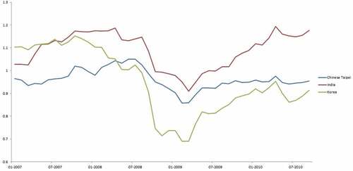
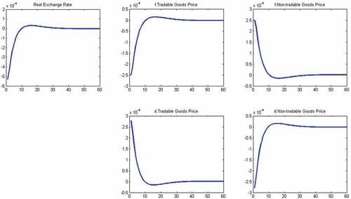
Domestic output, investment and asset prices fall are the typical results following a credit crunch. What is interesting here is the movement of resources across sectors and the dynamics of the real exchange rate. The international loan is denominated in tradable goods. When the loans that foreign banks made to domestic banks suddenly decrease, in the foreign country, the demand for tradable goods decreases and the price of tradables relative to non-tradables decreases. In the domestic country, the supply of tradable goods suddenly decreases, which increases the price of tradables relative to non-tradables. As a result, the real exchange rate decreases on impact. Over time, in the domestic country, labor and investment move from the non-tradable to the tradable sector to equalize the prices in two sectors, the exchange rate appreciates toward its steady state value. Figure 13 plots the impulse responses of real exchange rate and price of tradable and non-tradable goods in the foreign and domestic countries. Figure 8 documents the real exchange rate movements of Chinese Taipei, India and Korea. The sharp reduction in the real exchange rate of these countries against the U.S. happened around the time when U.S. banks substantially deleveraged their balance sheet with respect to Asia.

Figure 8. Real exchange rate movements of emerging markets.Source: Bank for International Settlement (2012)

Figure 14 plots the impulse responses of repayment shock under different values of ${\gamma }_f$. A lower value of ${\gamma }_f$ can be interpreted as banks’ strategy to contract foreign loans and give priority to long-term domestic borrowers. Peek and Rosengren (1997) documented this behavior among Japanese banks. It can also be interpreted as a lower credit rating of the domestic economy. With a smaller ${\gamma }_f$, the repayment shock generates much larger volatilities of domestic variables while decreasing the volatilities of foreign variables. In other words, a lower ${\gamma }_f$ helps mitigate the effects of the financial shock in the developed country where it originates, while amplifying the effects on the developing country. The intuition for this comes from foreign banks’ capital requirement constraint:

$d_t^{\ast }\le {\gamma }_e{l}_{e,t}^{\ast }+{\gamma }_i{l}_{i,t}^{\ast }+{\gamma }_f{p}_t^{T\ast }{l}_{f,t}$

.

Since deposit equals assets minus equity

$l_{i,t}^{\ast }+l_{e,t}^{\ast }+p_t^{T\ast }{l}_{f,t}-E_t^{\ast }\le {\gamma }_e{l}_{e,t}^{\ast }+{\gamma }_i{l}_{i,t}^{\ast }+{\gamma }_f{p}_t^{T\ast }{l}_{f,t}$

,

(26) $\left(1-{\gamma }_e\right)l_{e,t}^{\ast }+\left(1-{\gamma }_i\right)l_{i,t}^{\ast }+\left(1-{\gamma }_f\right)p_t^{T\ast }{l}_{f,t}\le E_t^{\ast }$(26)

When default happens and decreases foreign banks’ equity, $E_t^{\ast }$, these banks will have to decrease the left hand side of the above equation. When ${\gamma }_f$ is smaller than ${\gamma }_i,{\gamma }_e$, it is more beneficial for the foreign banks to contract international loans. One unit decrease in $l_{f,t}$ will loosen the capital requirement constraint by $1-{\gamma }_f$, which is larger than $1-{\gamma }_e$, or $1-{\gamma }_i$, if banks contract business loans, or consumer loans. The adjustment costs banks face are convex and together with $\gamma$ will determine how banks contract their portfolios. Without the convexity in costs, when ${\gamma }_f$ is lower relative to ${\gamma }_i$ and ${\gamma }_e$, banks will find it most beneficial to contract foreign loans only.

Devereux and Yetman (2010), using the data for the recent crisis, found that the magnitude of capital flow from one country to the U.S. depends on the country’s foreign currency credit rating. A lower rating resulted in a larger capital outflow of the country to the U.S., following the recent U.S. crisis. A lower rating asset will have a higher weight in banks’ risk weighted asset (RWA) portfolio in equation 26(26) $\left(1-{\gamma }_e\right)l_{e,t}^{\ast }+\left(1-{\gamma }_i\right)l_{i,t}^{\ast }+\left(1-{\gamma }_f\right)p_t^{T\ast }{l}_{f,t}\le E_t^{\ast }$(26) , or a lower ${\gamma }_f$ in our model. Thus, the empirical evidence is in line with our model prediction that countries perceived as more risky will suffer more from the U.S. crisis than less risky countries.

4.2. ${\gamma }_f$ Shock

4.2.1. Permanent shock

A permanent shock to ${\gamma }_f$ can be interpreted as a change in regulation. A real-world example of this is the change from the Basel I Accord to the Basel II Accord. Under the Basel I Accord, banks’ assets were classified into categories such as sovereign, banks, collateral, etc. All debts under the same category carried the same weight in banks’ RWA and banks were required to hold capital equal to 8% of banks’ total RWA. For example, all corporate debts had the weight of 100% and all government debts had the weight of 0%. The Basel II Accord no longer gives the same weight to all assets in one category if they have a different level of risks. Borrowing banks in developing countries, if considered risky by Basel II’s new assessment of risk, will have a higher weight in the lending bank’s RWA.

Figures 15 to 18 have impulse response for a 10% permanent negative shock to ${\gamma }_f$. As the international inter-bank loan has a higher weight in the lending banks’ RWA, lending banks permanently increase the lending rate, $R_f$, and decrease the amounts of loans made to borrowing banks in the developing country, $l_f$. The steady state interbank lending rate is: $R_f=\frac{1}{{{\beta }_B}^{\ast }}-\left[\frac{1}{{{\beta }_B}^{\ast }}-\frac{1}{{{\beta }_H}^{\ast }}\right]{\gamma }_f$. When ${\gamma }_f$ decreases, $R_f$ converges to a higher steady state. The steady state lending rates to domestic borrowers are the weighted average of interbank lending rate and domestic deposit rate. Thus, they converge to a new higher steady state. As a result, domestic consumption, output and investment converge to a lower steady state.

As ${\gamma }_f$ permanently decreases, from equation 25(25) $d_t^{\ast }\le {\gamma }_e{l}_{e,t}^{\ast }+{\gamma }_i{l}_{i,t}^{\ast }+{\gamma }_f{p}_t^{T\ast }{l}_{f,t}$(25) , we see that foreign banks’ capital requirement constraint tightens. Foreign banks can “loosen” the constraint by either deleveraging (reducing the total size of its RWA and deposit) or restructuring its portfolio (holding less assets with high weight and more assets with low weight). The foreign banks’ adjustment cost helps pin the optimal path for their deposit demand and loan supply. Contrary to the repayment shock, when the only option is to deleverage, foreign banks in this case also restructure their portfolios and hold more assets with lower weight in their RWA. As a result, foreign deposit goes down (deleverage effect) and loans to foreign HHs and entrepreneurs go up (portfolio restructuring effect). The foreign investment, consumption and output go up. New steady state foreign domestic lending rates, which only depend on foreign banks and patient HHs time preference, stay the same.

4.2.2. Temporary shock

Figures 19–22 have the impulse responses for the temporary negative shock to ${\gamma }_f$. The temporary shock can be interpreted as an exogenous temporary drop in domestic banks’ credit rating. A real-world example for this is the drop in domestic bank credit rating of South Korean banks during the Asian financial crisis in 1997. Figure 9 has the graph of credit ratings of nationwide South Korean banks and the South Korean Won—US Dollar exchange rate. Credit Ratings of major banks in South Korea dropped significantly before and right at the beginning of the crisis. The results of the impulse response show a drop in domestic gdp, consumption and investment. The foreign loan given to domestic banks contracts and interest rate increases. The real exchange rate also depreciates as a result of tightening foreign credit. This was also the experience of South Korea during the financial crisis.

Figure 9. S. Korean won/USD exchange rate and major S. Korean banks rating.Source: Moody’s (2012)

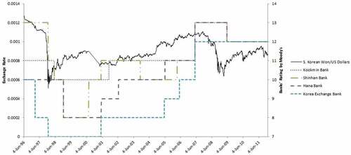
Figure 10. Impulse response: foreign repayment shock.Source: Matlab output

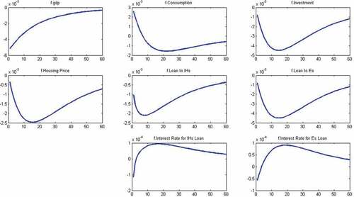
Figure 11. Impulse response: foreign repayment shock (cont.).Source: Matlab output

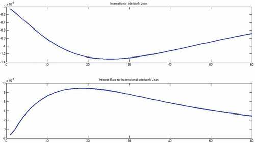
Figure 12. Impulse response: foreign repayment shock (cont.).Source: Matlab output

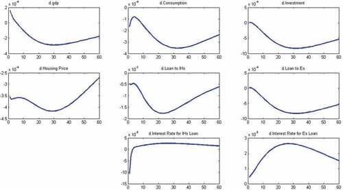
Figure 13. Impulse response: foreign repayment shock (cont.).Source: Matlab output

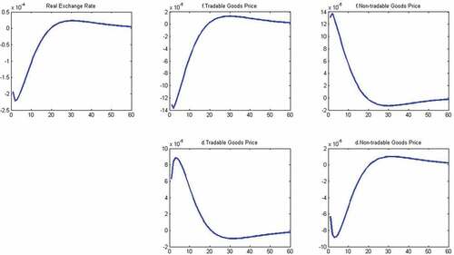
Figure 14. Impulse response: foreign repayment shock (cont.).Source: Matlab output

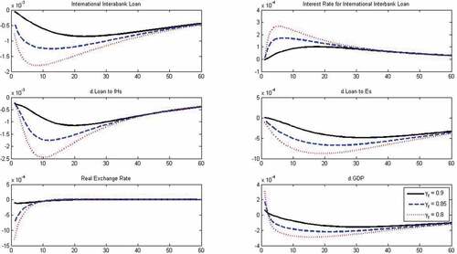
Figure 15. Impulse response: permanent shock to ${\gamma }_f$.Source: Matlab output

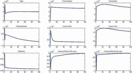
Figure 16. Impulse response: permanent shock to ${\gamma }_f$ (cont.).Source: Matlab output

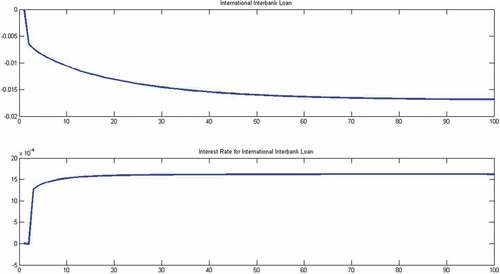
Figure 17. Impulse response: permanent shock to ${\gamma }_f$ (cont.).Source: Matlab output

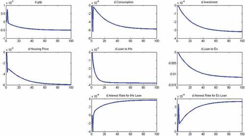
Figure 18. Impulse response: permanent shock to ${\gamma }_f$ (cont.).Source: Matlab output

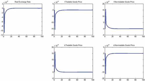
Figure 19. Impulse response: temporary shock to ${\gamma }_f$.Source: Matlab output

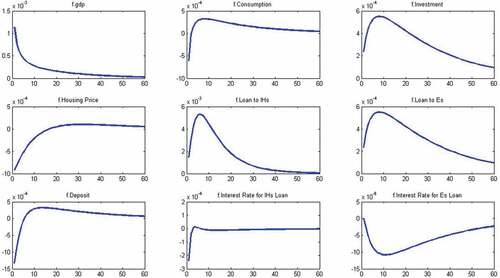
Figure 20. Impulse response: temporary shock to ${\gamma }_f$ (cont.).Source: Matlab output

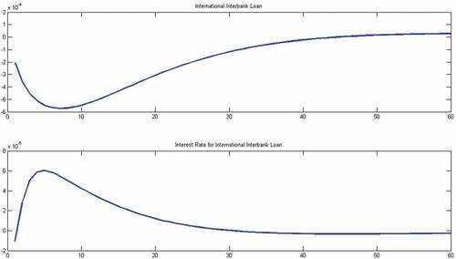
Figure 21. Impulse response: temporary shock to ${\gamma }_f$ (cont.).Source: Matlab output

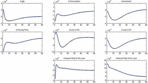
Figure 22. Impulse response: temporary shock to ${\gamma }_f$ (cont.).Source: Matlab output

5. Relation to empirical facts and existing literature

For the foreign repayment shock, our model generates a drop in output, consumption, investment, loans and housing prices and an increase in bank lending rates in both home and foreign countries. The borrowing country’s real exchange rate also depreciates. Qualitatively, our model matches the empirical facts. The lowest drop in the foreign and domestic consumption are 2*10⁻³ and 2*10⁻⁴, respectively. The drops of foreign and domestic investment are 5*10⁻³ and 5*10⁻⁴. The transmission of shock to the foreign country is just 10%. Quantitatively, our model does not match the magnitude of international transmission observed in data.

Devereux and Yetman (2010) built an international portfolio model to describe the recent crisis. Leveraged investors in each country holds foreign equity in their portfolios. The total value of their portfolios has to be greater than a constant times their equities. When a shock hits the home country and decreases home asset prices, the value of portfolios of home and foreign investors decreases, forcing them to deleverage. Eric van Wincoop (2011) built a model with leveraged financial institutions, who invest in both home and foreign assets. The default shock in his model is similar to the repayment shock in ours. Since foreign financial institutions hold domestic assets, the domestic default shock damages the foreign bank balance sheet and spreads the crisis to the foreign country. The main difference between our model and theirs is in our model, the leveraged domestic bank does not hold foreign asset. In our model, shock is transmitted through a credit crunch in the interbank loan market. Their models fit well for the comovement between the U.S. and Europe since European Banking Centers were the majority foreign holders of U.S. MBS. Our model fits the story between the U.S. and EAM. EAM were not directly exposed to the U.S. MBS as only 3% of U.S. MBS are held outside of the U.S., Europe and the Caribbean.

Ueda (2010), Kollmann et al. (2011) and Kalemli-Ozcan et al. (2012) also build international business cycle models with leveraged bank(s). In those models, borrowers in both countries borrow from a common lender(s). When shock hits one country and damages the balance sheet of the common lender(s), the common lender(s) contract loans in both countries. In their model, borrowers in one country have direct access to the credit of the foreign lenders. The story works in the developed world. For EAM, this is not the case as few borrowers in EAM have direct access to U.S. bank credit. In our model, borrowers in EAM only borrow funds from the U.S. through domestic banks. Thus, in steady state, banks in EAM are net borrowers in our model, which is an empirical fact and cannot be generated with a model of two symmetric countries.

Another main difference between our model and previous models with leveraged financial investors (banks) is in our capital requirement (leverage) constraint, we separate the weights of different assets in the lending bank RWA. Thus, we are able to investigate the behavior of international transmission of shock when borrowing banks have different credit ratings. We found that when the borrowing economy has a lower rating, the magnitude of capital that flows back to the U.S. in the crisis is higher. Our result is consistent with the empirical findings in Devereux and Yetman (2010).

6. Conclusion

The recent financial crisis in the U.S. highlights the role that the banking sector plays in the global macroeconomy. There has been substantial empirical evidence that suggests financial crisis can be transmitted across borders through the contraction in cross-border loans in the banking system. The very first empirical papers were written by Peek and Rosengren (1997; 2000), who studied the Japanese financial crisis and its effects on the U.S. More recent empirical papers study the U.S. financial crisis and its effects on lending in other countries. Such papers are Cetorelli & Goldberg, 2012 and Cetorelli & Goldberg, 2009) and Popov and Udell (2010). Our model provides a theoretical framework to support the hypothesis. When financial shock hits one country, the cross-border inter-bank loan contracts and transmits the shock to another country.

Our paper is also related to a number of papers that study the effects of shocks to international lending rates on a small open economy. These include Buyukkarabacak (2008), Christensen et al. (2016), and Faia and Iliopulos (2011). These papers treat the source of shock as exogenous. Our paper goes one step further and points out that the lending country’s financial shock could be what is behind the increase in the international lending rate. Our paper also differs from other recent papers with leveraged banks (investors) in three dimensions. First, the shock from the source country is not directly transmitted by damaging the foreign banks’ balance sheet, but rather, from contracting the loan in the interbank market. This helps apply our model for EAM, which were not directly exposed to the U.S. MBS. Second, borrowers in one country do not borrow directly from foreign banks, but through domestic banks. Thus, in the steady state, at the banking level, EAM are net borrowers from the U.S. Third, we separate the weight of international loans from weights for consumer and business loans in the capital requirement constraint. This helps us investigate the dynamics of the borrowing country when its banks have different credit ratings and when there is a bank regulation change in the lending country.

7. Recommendations

Our paper suggests policy directions on how best to react to global financial crisis. Firstly, when the credit crunch is the result of rising non-performing loans and tightening capital requirement regulation for banks, central banks could consider loosening the capital requirement to avoid the propagation of negative financial shock. In addition, central banks can lower policy rates to avoid credit crunch in global interbank market. A quantitative exercise of such policies is worth to be studied in the future. Secondly, major economies (U.S., Euro Area, Japan) could offer currency swap to support credit for emerging markets to mitigate the effects of the credit crunch. Such policy is beneficial and poses little cost or risk, as the credit crunch originates from major economies rather than being caused by weakness in the financial system of emerging markets. The U.S. Federal Reserves currently has Dollar liquidity swap lines with 14 other countries. Most are developed countries rather than emerging markets (except for Mexico, Brazil and South Korea). Further expanding currency liquidity swap lines could be beneficial for global financial stability. Thirdly, emerging markets should diversify its bank funding sources and strengthen the balance sheet of banks to reduce negative impacts from financial shocks originated from major countries.

Disclosure statement

No potential conflict of interest was reported by the author(s).

Additional information

Funding

The authors received no direct funding for this research.

Notes on contributors

Hoang Tuan Dao

Dao Hoang Tuan holds a Ph.D in Economics from Boston College (2013). He is now an Assistant Professor at Academy of Policy and Development, Hanoi, Vietnam. His research interests include international finance, financial structure and economic growth, and foreign direct investment. He has worked on policy consultative projects with the World Bank, UNDP and Foreign Investment Agency, Ministry of Planning and Investment, Vietnam.

Taesu Kang

Taesu Kang holds a Ph.D in Economics from Boston College (2012). He is now a Senior Economist at Bank of Korea. His research interest include international finance, monetary policy and labor market. He has published in Journal of International Economics and Economic Analysis (Quarterly).

Notes

1. We thank Fabio Ghironi for helpful comments on earlier drafts of the manuscript.

2. Kamin and DeMarco (2012) document that the majority of foreign exposure to U.S. MBS are of European Banking Centers.

3. The model is built upon Iacoviello and Neri (2015) closed economy model.

References

- Backus, D. K., Kehoe, P. J., & Kydland, F. E. (1994). Dynamics of the trade balance and the terms of trade: The j-curve? American Economic Review, 84(1), 84–23 https://EconPapers.repec.org/RePEc:aea:aecrev:v:84:y:1994:i:1:p:84-103.
- Buyukkarabacak, B. (2008). Consumption volatility in emerging economies: credit constraints, collateral and income distribution. PhD thesis. Emory University.
- Campbell, J. Y., & Mankiw, N. G. (1990). Permanent income, current income, and consumption. Journal of Business and Economic Statistics, 8(3), 265–279 https://econpapers.repec.org/article/besjnlbes/v_3a8_3ay_3a1990_3ai_3a3_3ap_3a265-79.htm.
- Cetorelli, N., & Goldberg, L. S. (2009). Globalized banks: Lending to emerging markets in the crisis. Technical report (Federal Reserve Bank of New York).
- Cetorelli, N., & Goldberg, L. S. (2012). Banking globalization and monetary transmission. The Journal of Finance, 67(5), 1811–1843. https://doi.org/10.1111/j.1540-6261.2012.01773.x
- Christensen, I., Corrigan, P., Mendicino, C., & Nishiyama, S.-I. (2016). Consumption, housing collateral, and the Canadian business cycle. Canadian Journal of Economics, 49(1), 207–236. https://doi.org/10.1111/caje.12195
- Devereux, M. B., & Yetman, J. (2010). Leverage constraints and the international transmission of shocks. Journal of Money, Credit, and Banking, 42(s1), 71–105. https://doi.org/10.1111/j.1538-4616.2010.00330.x
- Dib, A. (2010a). Banks, credit market frictions, and business cycles. Technical report (Bank of Canada).
- Dib, A. (2010b). Capital requirement and financial frictions in banking: Macroeconomic implications. Technical report (Bank of Canada).
- Faia, E., & Iliopulos, E. (2011). Financial openness, financial frictions and optimal monetary policy. Journal of Economic Dynamics & Control, 35(11), 1976–1996. https://doi.org/10.1016/j.jedc.2011.06.012
- Forlati, C. & Lambertini, L. (2011). Risky Mortgages in a DSGE Model. International Journal of Central Banking, 7(1), 285–335.
- Gertler, M., & Kiyotaki, N. (2010). Financial intermediation and credit policy in business cycle analysis. Handbook of Monetary Economics, 3, 547–599 https://www.sciencedirect.com/science/article/abs/pii/B9780444532381000119.
- Iacoviello, M. (2005). House prices, borrowing constraints, and monetary policy in the business cycle. American Economic Review, 95(3), 739–764. https://doi.org/10.1257/0002828054201477
- Iacoviello, M. (2015). Financial business cycle. Review of Economic Dynamics, 18(1), 140–163. https://doi.org/10.1016/j.red.2014.09.003
- Imai, M., & Takarabe, S. (2011). Bank integration and transmission of financial shocks: Evidence from Japan. American Economic Journal: Macroeconomics, 3(1), 155–183 https://www.jstor.org/stable/41237135.
- Kalemli-Ozcan, S. & Papaioannou, E. & Perri, F. (2012). Global Banks and Crisis Transmission. Journal of International Economics, 89(2), 495–510.
- Kamin, S. B., & DeMarco, L. P. (2012). How did a domestic housing slump turn into a global financial crisis? Journal of International Money and Finance, 31(1), 10–41. https://doi.org/10.1016/j.jimonfin.2011.11.003
- Kiyotaki, N., & Moore, J. (1997). Credit cycles. Journal of Political Economy, 105(2), 211–248. https://doi.org/10.1086/262072
- Kollmann, R., Enders, Z., & Mller, G. J. (2011). Global banking and international business cycles. European Economic Review, 55(3), 407–426. https://doi.org/10.1016/j.euroecorev.2010.12.005
- Peek, J., & Rosengren, E. S. (1997). The international transmission of financial shocks: The case of Japan. American Economic Review, 87(4), 495–505 https://www.jstor.org/stable/2951360.
- Peek, J., & Rosengren, E. S. (2000). Collateral damage: Effects of the japanese bank crisis on real activity in the United States. American Economic Review, 90(1), 30–45. https://doi.org/10.1257/aer.90.1.30
- Popov, A., & Udell, G. F. (2010). Cross-border banking and the international transmission of financial distress during the crisis of 2007-2008. Working Paper Series 1203, European Central Bank.
- Stockman, A. C., & Tesar, L. L. (1995). Tastes and technology in a two-country model of the business cycle: Explaining international comovements. American Economic Review, 85(1), 168–185 https://www.jstor.org/stable/2118002.
- Ueda, K. (2010). Banking globalization and international business cycles. Technical report (Bank of Japan).
- Wincoop, E. (2011). International contagion through leveraged financial institutions. NBER Working Papers 17686, National Bureau of Economic Research, Inc.