Innovation-Based Research Using Structural Flexibility and Acceptance Model (SFAM)

Abstract

The research objectives are as follows: (1) Develop a solid structural model assuming normality and homoscedasticity. (2) Obtain the property estimator of the flexible and robust SFAM structural model. (3) Obtaining hypothesis testing of each relationship built from the flexible and strong SFAM structural model. This research is integrated with a flexible and robust modeling approach based on nonparametric smooth spline regression analysis (RNSS) that can capture the shape and robustness of relationships dependent on empirical data. There are at least three transformation methods namely SRS, MSI and RASCH that will be used in SFAM development. The results obtained are the development of a flexible structural model in the form of relationships between variables and a robust structural model from the two assumptions, then the estimator properties and hypothesis testing of each relationship are built from the two models. The authenticity of this research is very evident in the discovery of a new model, namely SFAM that can accommodate various things, which are the weaknesses of various existing analytical tools such as recursive and recursive models, more than one endogenous variable, flexible and strong models.

Keywords:

• Flexible and Sturdy Structural Modeling
• SFAM
• SEM

1. Introduction

This study will reconstruct the Structural Flexibility and Acceptance Model (SFAM) as the stage of developing a concept/theory/proposal regarding statistical modeling. The meaning of the 4 words in the model are as follows: structural reflects the structural model that has been built, flexibility indicates a flexible model, acceptance implies a strong and hypothesis-free model (Fernandes, 2018). reconstruction or statistical model based on stochastic. The novelty of this research can be seen in the discovery of a new model, namely SFAM which can handle several things, which is the weakness of several existing analytical tools such as recursive and recursive models. Frequently used statistical models, such as SEM, PLS, GSCA and WarpPLS, have drawbacks and can be handled using SFAM (Fernandes, 2017). This system modeling is a very broad data analysis method, especially in the social, humanistic and educational fields, in research using a quantitative approach.

Quantitative, qualitative and mixed methods research approaches in various fields are developing very rapidly. For example, research in the field of accounting that started using a quantitative approach, is now starting to shift to a qualitative approach, this is after the development of behavioral accounting (Fernandes et al., 2014). Likewise in the economic field. Such as the social and humanities fields that have developed earlier, for example sociometry, psychometry and econometrics. Research with a quantitative approach in the social and humanities field is not an interesting thing at first, because researchers often have difficulty in analyzing data. The application of statistics as a data analysis method in general can be difficult for them. However, with the development of computing tools in the form of computer machines, this problem can be overcome. Research in the social humanities generally investigates systems, where one of the characteristics of the system is very complex (Purbawangsa et al., 2019). Simplification of the solution can be done through modeling, one of which is modeling using statistics. The main characteristic of statistical modeling is the existence of a relationship between variables and the nature of the relationship is stochastic. In other words, model design always begins with the formulation of research hypotheses.

Theories and results of previous research can be used as a basis for thinking for further research. In designing the relationship between variables in a model based on the construction of hypotheses. The disruption effect, which brings the logic of future thinking to current research, is one of the answers to a current problem. We can follow disruptive innovation when the foundation or perspective of research thinking, namely in structuring the relationship between variables in the model, is developed as follows: (1) Finality norms (scriptures), (2) axioms, (3) theorems/theories/propositions, (4) Results of empirical research, (5) Adoption of theory and/or results of empirical research on the relationship between variables from other fields of science, (6) Non-final norms, such as government regulations, laws, SOPs, and so on, (7) Conditions empirical, (8) Expert judgment, and (9) Intuition/logic. Elements (1), (6) to (9) allow us to build or reconstruct the model through theory (Fernandes et al., 2019). New research (new ideas/ideas) can be more easily obtained from local wisdom if the basis or perspective of research thinking can be expanded in such a way so that it can encourage the development of indigenous knowledge.

The nature of research subjects in the social humanities field is changing rapidly and dynamically. System modeling based on innovation which is seen as being able to keep up with rapid and dynamic changes is also capable of capturing future phenomena. Thus, it is hoped that today's researchers, students and lecturers are not limited to existing theories, but can carry out scientific constructions even though they use quantitative research.

This research is an effort to socialize the latest ideas. With disruptive innovation, the main emphasis is on impacting what we produce and on life, both scientific life and people's lives. System modeling analysis that has developed and is often used includes Structural Equation Modeling (SEM). Until now, there have been several SEM analyzes whose applications have developed in Indonesia, including SEM with AMOS/LISREL software, PLS using SmartPLS software, GSCA with GeSCA and WarpPLS software.

Modeling involves latent variables, where the data analyzed are generally obtained by measuring the process using a questionnaire. The questionnaire was applied using a Likert scale model, and produced data in the form of scores. In general, the weakness of all these methods is that they do not include the concept of data transformation in the form of scores into the scale. So it is necessary to develop a model that can include the concept of data transformation in the form of scores into scales. There are at least three transformation methods, namely using SRS, MSI, and RASCH which will be used to complement the modeling method, by developing a Structural Flexibility and Acceptance Model (SFAM).

The Structural Flexibility and Acceptance (SFAM) Reconstruction Model is equipped with the concept of path analysis with categorical data so that it can also be used to analyze categorical data. On the other hand, the development of SFAM is also equipped with a flexible and robust model approach based on nonparametric smoothing spline regression analysis (RNSS) which can capture the form of relationships that depend on empirical data. This study aims to describe the modeling of a flexible and robust structure, the realization of a new model, namely Structural Flexibility and Acceptance (SFAM). This study aims to: (5) Develop a flexible structural model on the relationship between variables. (6) Develop a structural model that is robust against the assumptions of normality and homoscedasticity. (7) obtain a property estimator from a flexible and robust SFAM structural model. (8) Obtaining hypothesis testing of each relationship built from the flexible and robust SFAM structural model.

This research was conducted to reconstruct Structural Flexibility and Acceptance (SFAM), which is a structural model that is strong in handling linearity assumptions, or in other words, a structural model that can accommodate non-linear relationships between variables. and strong on the distribution assumption and the assumption of homoscedasticity. Apart from that, SFAM is also equipped with useful power for analyzing categorical data.

2. Result and discussion

2.1. Development of a flexible structural model in relationship between variables

Regression analysis is a function that relates exogenous variables (X) to endogenous variables (Y) which can be in the form of linear or nonlinear relationships (Fernandes and Taba, 2018). Simple linear regression analysis has one exogenous variable and one endogenous variable with the form of a relationship that can be described as a straight line. While simple quadratic regression analysis is a function of one endogenous variable and one exogenous variable that has the highest rank with a value of two, so that the form of the relationship can be described as a parabolic line (Fernandes, 2017). Path analysis is an extension of multiple regression analysis, where there is one exogenous variable and two endogenous variables involved, namely the intervening endogenous variable (Y1) and the pure endogenous variable (Y2) which can be described below. path analysis model in Figure 1.

Figure 1. path analysis diagram.

Path analysis can also describe the pattern of relationships between variables that are linear and also nonlinear (Sumardi and Fernandes, 2020). Quadratic path analysis involves one exogenous and one intervening variable with endogenous m = 2, and one pure endogenous variable of order m = 1. While complex linear path analysis involves one exogenous variable with q endogenous variables. All variables in complex linear path analysis have an order of m = 1. Thus, a complex quadratic path analysis model can be made with all variables having an order of m = 2. The path analysis model can be further expanded by adding an order of m for each exogenous intervening variable and endogenous so that it can produce a simple m order path analysis model (with 2 endogenous variables) and complex m order path analysis (endogenous variable q-1 and endogenous intervening variable q-1).    

Lemma 2.1 Form of simple quadratic path analysis model

If given paired data ($X_i,Y_{1i},Y_{2i}$) with $i=1,2,3,\dots ,n$ following the quadratic path analysis model, the quadratic path analysis function is obtained as presented in equation (2.1.1) and the model in (2.1.2)

(2.1.1) $\begin{array}{rl}& Y_{1i}=f(X_i,X_i^2)+{\epsilon }_{1i}\\ & Y_{2i}=f(X_i,X_i^2,Y_{1i},Y_{1i}^2)+{\epsilon }_{2i}\end{array}$(2.1.1)

(2.1.2) $\begin{array}{rl}& Y_{1i}={\beta }_{011}+{\beta }_{111}{X}_i+{\beta }_{211}{X}_i^2+{\epsilon }_{1i}\\ & Y_{2i}={\beta }_{012}+{\beta }_{112}{X}_i+{\beta }_{212}{X}_i^2+{\beta }_{122}{Y}_{1i}+{\beta }_{222}{Y}_{1i}^2+{\epsilon }_{2i}\end{array}$(2.1.2)

Matrix form

$\underset{\sim 2n\times 1}{Y}={\mathbf{X}}_{{ }_{2n\times 8}}\underset{\sim 8\times 1}{\beta }+\underset{\sim 2n\times 1}{\epsilon }$

Proof:

Before obtaining the model in the Simple Quadratic Path Analysis, the first model is obtained from (a) Simple Linear Regression Analysis; (b) Simple Linear Path Analysis; and (c) Quadratic Regression Analysis as follows:

First part: Find out the simple linear regression model with equation (2.1.3) and the model in (2.1.4).

(2.1.3) $Y_{1i}=f(X_i)+{\epsilon }_{1i}$(2.1.3)

(2.1.4) $Y_i={\beta }_0+{\beta }_1{X}_i+{\epsilon }_i$(2.1.4)

The matrix can be formed:

$Y_{\sim n\times 1}={\mathbf{X}}_{{ }_{n\times 2}}{\beta }_{\sim 2\times 1}+{\epsilon }_{\sim n\times 1}$

$\left[\begin{array}{c}{Y}_1\\ Y_2\\ Y_3\\ ⋮\\ Y_n\end{array}\right]=\left[\begin{array}{cc}1& X_1\\ 1& X_2\\ 1& X_3\\ ⋮& ⋮\\ 1& X_n\end{array}\right]\left[\begin{array}{c}{\beta }_0\\ {\beta }_1\end{array}\right]+\left[\begin{array}{c}{\epsilon }_1\\ {\epsilon }_2\\ {\epsilon }_3\\ ⋮\\ {\epsilon }_n\end{array}\right],$

where:

$Y_i:$ Endogenous variable of the i-th observation ($i=1,2,3,\dots ,n$);

$X_i:$ Exogenous variable of the i-th observation;

$n:$ The number of observations;

${\beta }_j:$ The coefficient of influence of exogenous variables on endogenous ($j=0,1,2$);

${\epsilon }_i:$ Random error of the i endogenous variable

Part Two: Find a simple linear path analysis model as presented in equation (2.1.5) and the model in (2.1.6).

(2.1.5) $\begin{array}{rl}& Y_{1i}=f(X_i)+{\epsilon }_{1i}\\ & Y_{2i}=f(X_i,Y_{1i})+{\epsilon }_{2i}\end{array}$(2.1.5)

(2.1.6) $\begin{array}{rl}& Y_{1i}={\beta }_{01}+{\beta }_{11}{X}_i+{{\epsilon }_1}_i\\ & Y_{2i}={\beta }_{02}+{\beta }_{12}{X}_i+{\beta }_{22}{Y}_{1i}+{\epsilon }_{2i}\end{array}$(2.1.6)

The following matrix can be formed:

$Y_{\sim 2n\times 1}={\mathbf{X}}_{{ }_{2n\times 5}}{\beta }_{\sim 5\times 1}+{\epsilon }_{\sim 2n\times 1}$

Part Three: After knowing the equations and simple linear regression models, a simple quadratic regression model can be made as presented in equations (2.1.7) and (2.1.8).

(2.1.7) $Y_i=f(X_i,X_i^2)+{\epsilon }_i$(2.1.7)

(2.1.8) $Y_i={\beta }_0+{\beta }_1{X}_i+{\beta }_2{X}_i^2+{\epsilon }_i$(2.1.8)

The matrix form of the model is:

$Y_{\sim n\times 1}={\mathbf{X}}_{{ }_{n\times 3}}{\beta }_{\sim 3\times 1}+{\epsilon }_{\sim n\times 1}$

$\left[\begin{array}{c}{Y}_1\\ Y_2\\ Y_3\\ ⋮\\ Y_n\end{array}\right]=\left[\begin{array}{cc}1& X_1\\ 1& X_2\\ 1& X_3\\ ⋮& ⋮\\ 1& X_n\end{array}\begin{array}{c}{X}_1^2\\ X_2^2\\ X_3^2\\ ⋮\\ X_n^2\end{array}\right]\left[\begin{array}{c}{\beta }_0\\ {\beta }_1\\ {\beta }_2\end{array}\right]+\left[\begin{array}{c}{\epsilon }_1\\ {\epsilon }_2\\ {\epsilon }_3\\ ⋮\\ {\epsilon }_n\end{array}\right]$

where:

$Y_i:$ Endogenous variable of the i-th observation ($i=1,2,3,\dots ,n$);

$X_i:$ Exogenous variable of the i-th observation;

$X_i^2:$ Exogenous variable to the power of 2 (squared) of the i-th observation;

$n:$ The number of observations;

$q:$ The number of exogenous variables;

${\beta }_j:$ The coefficient of influence of exogenous variables on endogenous ($j=0,1,2$);

${\epsilon }_i:$ Random error of the i endogenous variable

From the equations in the simple linear regression analysis model, simple path analysis, and quadratic regression analysis that has been described, a function that is formed as in equations (2.1.1) and (2.1.2) can be obtained, so that the following matrix is obtained:

$Y_{\sim 2n\times 1}={\mathbf{X}}_{{ }_{2n\times 8}}{\beta }_{\sim 8\times 1}+{\epsilon }_{\sim 2n\times 1}$

$\left[\begin{array}{c}{Y}_{11}\\ Y_{12}\\ Y_{13}\\ ⋮\\ Y_{1n}\\ Y_{21}\\ Y_{22}\\ Y_{23}\\ ⋮\\ Y_{2n}\end{array}\right]=\left[\begin{array}{cc}{\mathbf{X}}_{X{X}^2}& {\mathbf{0}}_{n\times 5}\\ {\mathbf{0}}_{n\times 3}& {\mathbf{X}}_{X{X}^{2}Y{Y}^2}\end{array}\right]\left[\begin{array}{c}{\beta }_{011}\\ {\beta }_{111}\\ {\beta }_{211}\\ {\beta }_{012}\\ {\beta }_{112}\\ {\beta }_{212}\\ {\beta }_{122}\\ {\beta }_{222}\end{array}\right]+\left[\begin{array}{c}{\epsilon }_{11}\\ {\epsilon }_{12}\\ {\epsilon }_{13}\\ ⋮\\ {\epsilon }_{1n}\\ {\epsilon }_{21}\\ {\epsilon }_{22}\\ {\epsilon }_{23}\\ ⋮\\ {\epsilon }_{2n}\end{array}\right]$

Lemma 2.2 Form of complex quadratic path analysis model

If given paired data ($X_i,Y_{1i},Y_{2i},Y_{3i},\dots ,Y_{(q-1)i},Y_{qi}$),equations and complex quadratic path analysis models can be made as presented in (2.2.1) and (2.2.2).

(2.2.1) $\begin{array}{rl}& Y_{1i}=f(X_i,X_i^2)+{\epsilon }_{1i}\\ & Y_{2i}=f(X_i,X_i^2,Y_{1i},Y_{1i}^2)+{\epsilon }_{2i}\\ & Y_{3i}=f(X_i,X_i^2,Y_{1i},Y_{1i}^2,Y_{2i},Y_{2i}^2)+{\epsilon }_{3i}\\ & ⋮\\ & Y_{(q-1)i}=f(X_i,X_i^2,Y_{1i},Y_{1i}^2,Y_{2i},Y_{2i}^2,\dots ,Y_{q-2,i},Y_{q-2,i}^2)+{\epsilon }_{(q-1)i}\\ & Y_{qi}=f(X_i,X_i^2,Y_{1i},Y_{1i}^2,Y_{2i},Y_{2i}^2,\dots ,Y_{q-1,i},Y_{q-1,i}^2)+{\epsilon }_{qi}\end{array}$(2.2.1)

(2.2.2) $\begin{array}{rl}& Y_{1i}={\beta }_{011}+{\beta }_{111}{X}_i+{\beta }_{211}{X}_i^2+{\epsilon }_{1i}\\ & Y_{2i}={\beta }_{012}+{\beta }_{112}{X}_i+{\beta }_{212}{X}_i^2+{\beta }_{122}{Y}_{1i}+{\beta }_{222}{Y}_{1i}^2+{\epsilon }_{2i}\\ & Y_{3i}={\beta }_{013}+{\beta }_{113}{X}_i+{\beta }_{213}{X}_i^2+{\beta }_{123}{Y}_{1i}+{\beta }_{223}{Y}_{1i}^2+{\beta }_{133}{Y}_{2i}+{\beta }_{233}{Y}_{2i}^2+{\epsilon }_{3i}\\ & ⋮\\ & Y_{(q-1)i}={\beta }_{01(q-1)}+{\beta }_{11(q-1)}{X}_i+{\beta }_{21(q-1)}{X}_i^2+{\beta }_{12(q-1)}{Y}_{1i}+{\beta }_{22(q-1)}{Y}_{1i}^2+{\beta }_{13(q-1)}{Y}_{2i}+{\beta }_{23(q-1)}{Y}_{2i}^2\\ & +\cdots +{\beta }_{1(q-1)(q-1)}{Y}_{q-2,i}+{\beta }_{2(q-1)(q-1)}{Y}_{q-2,i}^2+{\epsilon }_{(q-1)i}\\ & Y_{qi}={\beta }_{01q}+{\beta }_{11q}{X}_i+{\beta }_{21q}{X}_i^2+{\beta }_{12q}{Y}_{1i}+{\beta }_{22q}{Y}_{1i}^2+{\beta }_{13q}{Y}_{2i}+{\beta }_{23q}{Y}_{2i}^2+\cdots +{\beta }_{1qq}{Y}_{q-1,i}\\ & +{\beta }_{2qq}{Y}_{q-1,i}^2+{\epsilon }_{qi}\end{array}$(2.2.2)

With the form of a matrix:

$Y~qn\times 1=X_{qn\times (q+{\displaystyle {\sum }_{i=1}^{q}i})}\beta ~(q+{\displaystyle {\sum }_{i=1}^{q}i})\times 1+\epsilon ~qn\times 1$

Proof:

First part: The equations and models in the simple quadratic path analysis are known as shown in equations (2.2.3) and (2.2.4).

(2.2.3) $\begin{array}{rl}& Y_{1i}=f(X_i,X_i^2)+{\epsilon }_{1i}\\ & Y_{2i}=f(X_i,X_i^2,Y_{1i},Y_{1i}^2)+{\epsilon }_{2i}\end{array}$(2.2.3)

(2.2.4) $\begin{array}{rl}& Y_{1i}={\beta }_{011}+{\beta }_{111}{X}_i+{\beta }_{211}{X}_i^2+{\epsilon }_{1i}\\ & Y_{2i}={\beta }_{012}+{\beta }_{112}{X}_i+{\beta }_{212}{X}_i^2+{\beta }_{122}{Y}_{1i}+{\beta }_{222}{Y}_{1i}^2+{\epsilon }_{2i}\end{array}$(2.2.4)

The matrix form of the model is:

$Y~2n\times 1=X_{2n\times 8}\beta ~8\times 1+\epsilon ~2n\times 1$

Part Two: Equations and models in complex linear path analysis are shown in equations (2.2.5) and (2.2.6).

(2.2.5) $\begin{array}{rl}& Y_{1i}=f(X_i)+{\epsilon }_{1i}\\ & Y_{2i}=f(X_i,Y_{1i})+{\epsilon }_{2i}\\ & Y_{3i}=f(X_i,Y_{1i},Y_{2i})+{\epsilon }_{3i}\\ & ⋮\\ & Y_{qi}=f(X_i,Y_{1i},Y_{2i},\dots ,Y_{q-1,i})+{\epsilon }_{qi}\end{array}$(2.2.5)

(2.2.6) $\begin{array}{rl}& Y_{1i}={\beta }_{01}+{\beta }_{11}{X}_i+{\epsilon }_{1i}\\ & Y_{2i}={\beta }_{02}+{\beta }_{12}{X}_i+{\beta }_{22}{Y}_{11}+{\epsilon }_{2i}\\ & Y_{3i}={\beta }_{03}+{\beta }_{13}{X}_i+{\beta }_{23}{Y}_{21}+{\beta }_{33}{Y}_{22}+{\epsilon }_{3i}\\ & ⋮\\ & Y_{qi}={\beta }_{0q}+{\beta }_{1q}{X}_i+{\beta }_{2q}{Y}_{q1}+{\beta }_{3q}{Y}_{q2}+\cdots +{\beta }_{qq}{Y}_{q,q-1}+{\epsilon }_{qi}\end{array}$(2.2.6)

The matrix form of the model is:

$Y~qn\times 1=X_{qn\times (q+{\displaystyle {\sum }_{i=1}^{q}i})}\beta ~(q+{\displaystyle {\sum }_{i=1}^{q}i})\times 1+\epsilon ~qn\times 1$

From the results of the description of the model above, an extension of the model obtained in Lemma 3.1 can be made into a complex quadratic path analysis model following equation (2.2.1) and the model in (2.2.2), to obtain the following matrix form:

$Y~qn\times 1=X_{qn\times (q+{\displaystyle {\sum }_{i=1}^{q}i})}\beta ~(q+{\displaystyle {\sum }_{i=1}^{q}i})\times 1+\epsilon ~qn\times 1$

Lemma 2.3 Form of simple non-linear path analysis model (non-linear m-order)

If paired data ($X_i,Y_{1i},Y_{2i}$) with $i=1,2,3,\dots ,n$ follows a simple m-order path analysis model, equations and models can be obtained as presented in equations (2.3.1) and (2.3.2).

(2.3.1) $\begin{array}{rl}& Y_{1i}=f(X_i,X_i^2,X_i^3,\dots ,X_i^m)+{\epsilon }_{1i}\\ & Y_{2i}=f(X,X_i^2,X_i^3,\dots ,X^m,Y_{1i},Y_{1i}^2,Y_{1i}^3,\dots ,Y_{1i}^m)+{\epsilon }_{2i}\end{array}$(2.3.1)

(2.3.2) $\begin{array}{rl}& Y_{1i}={\beta }_{011}+{\beta }_{111}{X}_i+{\beta }_{211}{X}_i^2+\cdots +{\beta }_{m11}{X}_i^m+{\epsilon }_{1i}\\ & Y_{2i}={\beta }_{012}+{\beta }_{112}{X}_i+{\beta }_{212}{X}_i^2+\cdots +{\beta }_{m12}{X}_i^m+{\beta }_{122}{Y}_{1i}+{\beta }_{222}{Y}_{1i}^2+\cdots +{\beta }_{m22}{Y}_{1i}^m+{\epsilon }_{2i}\end{array}$(2.3.2)

The matrix form of the model is:

$Y~2n\times 1=X_{2n\times (3m+2)}\beta ~(3m+2)\times 1+\epsilon ~2n\times 1$

Proof:

Part One: The results of Lemma 2.1 have been obtained which are a form of the quadratic path analysis function as presented in equation (2.1.1) and the model in (2.1.2) with the following matrix form:

$Y~2n\times 1=X_{2n\times 8}\beta ~8\times 1+\epsilon ~2n\times 1$

$\left[\begin{array}{c}{Y}_{11}\\ Y_{12}\\ Y_{13}\\ ⋮\\ Y_{1n}\\ Y_{21}\\ Y_{22}\\ Y_{23}\\ ⋮\\ Y_{2n}\end{array}\right]=\left[\begin{array}{cc}{\mathbf{X}}_{X{X}^2}& {\mathbf{0}}_{n\times 5}\\ {\mathbf{0}}_{n\times 3}& {\mathbf{X}}_{X{X}^{2}Y{Y}^2}\end{array}\right]\left[\begin{array}{c}{\beta }_{011}\\ {\beta }_{111}\\ {\beta }_{211}\\ {\beta }_{012}\\ {\beta }_{112}\\ {\beta }_{212}\\ {\beta }_{122}\\ {\beta }_{222}\end{array}\right]+\left[\begin{array}{c}{\epsilon }_{11}\\ {\epsilon }_{12}\\ {\epsilon }_{13}\\ ⋮\\ {\epsilon }_{1n}\\ {\epsilon }_{21}\\ {\epsilon }_{22}\\ {\epsilon }_{23}\\ ⋮\\ {\epsilon }_{2n}\end{array}\right]$

From the results in Lemma 2.1, an expansion can be made by adding the order to m in the exogenous and endogenous intervening variables, so that equations and models are obtained as presented in equations (2.3.1) and (2.3.2) above with the following matrix form:

$Y~2n\times 1=X_{2n\times (3m+2)}\beta ~(3m+2)\times 1+\epsilon ~2n\times 1$

$\left[\begin{array}{c}{Y}_{11}\\ Y_{12}\\ Y_{13}\\ ⋮\\ Y_{1n}\\ Y_{21}\\ Y_{22}\\ Y_{23}\\ ⋮\\ Y_{2n}\end{array}\right]=\left[\begin{array}{cc}{\mathbf{X}}_{X^m}& {\mathbf{0}}_{n\times (2m+1)}\\ {\mathbf{0}}_{n\times (m+1)}& {\mathbf{X}}_{{(X{Y}_1)}^m}\end{array}\right]\left[\begin{array}{c}{\beta }_{011}\\ {\beta }_{111}\\ {\beta }_{211}\\ {\beta }_{311}\\ ⋮\\ {\beta }_{m11}\\ {\beta }_{012}\\ {\beta }_{112}\\ {\beta }_{212}\\ {\beta }_{312}\\ ⋮\\ {\beta }_{m12}\\ ⋮\\ {\beta }_{122}\\ {\beta }_{222}\\ {\beta }_{322}\\ ⋮\\ {\beta }_{m22}\end{array}\right]+\left[\begin{array}{c}{\epsilon }_{11}\\ {\epsilon }_{12}\\ {\epsilon }_{13}\\ ⋮\\ {\epsilon }_{1n}\\ {\epsilon }_{21}\\ {\epsilon }_{22}\\ {\epsilon }_{23}\\ ⋮\\ {\epsilon }_{2n}\end{array}\right]$

Lemma 2.4 Model shape non-linear complex path analysis (non-linear m-order)

If given paired data ($X_i,Y_{1i},Y_{2i},Y_{3i},\dots ,Y_{qi}$) with $i=1,2,3,\dots ,n$ which follows a complex non-linear path analysis model of order m, we can obtain the equations and models presented in equations (2.4.1) and (2.4.2)

(2.4.1) $\begin{array}{rl}& Y_{1i}=f(X,X^2,X^3,\dots ,X^m)+{\epsilon }_{1i}\\ & Y_{2i}=f(X,X^2,X^3,\dots ,X^m,Y_{1i},Y_{1i}^2,Y_{1i}^3,\dots ,Y_{1i}^m)+{\epsilon }_{2i}\\ & ⋮\\ & Y_{qi}=f(X,X^2,X^3,\dots ,X^m,Y_{1i},Y_{1i}^2,Y_{1i}^3,\dots ,Y_{1i}^m,\dots ,Y_{q-1,i},Y_{q-1,i}^2,Y_{q-1,i}^3,\dots ,Y_{q-1,i}^m)+{\epsilon }_{qi}\end{array}$(2.4.1)

(2.4.2) $\begin{array}{rl}& Y_{1i}={\beta }_{011}+{\beta }_{111}{X}_i+{\beta }_{211}{X}_i^2+\cdots +{\beta }_{m11}{X}_i^m+{\epsilon }_{1i}\\ & Y_{2i}={\beta }_{012}+{\beta }_{112}{X}_i+{\beta }_{212}{X}_i^2+\cdots +{\beta }_{m12}{X}_i^m+{\beta }_{122}{Y}_{1i}+{\beta }_{222}{Y}_{1i}^2+\cdots +{\beta }_{m22}{Y}_{1i}^m+{\epsilon }_{2i}\\ & ⋮\\ & Y_{qi}={\beta }_{01q}+{\beta }_{11q}{X}_i+{\beta }_{21q}{X}_i^2+\cdots +{\beta }_{m1q}{X}_i^m+{\beta }_{12q}{Y}_{1i}+{\beta }_{22q}{Y}_{1i}^2+\cdots +{\beta }_{m2q}{Y}_{1i}^m\\ & +\cdots +{\beta }_{1qq}{Y}_{q-1,i}+{\beta }_{2qq}{Y}_{q-1,i}^2+\cdots +{\beta }_{mqq}{Y}_{q-1,i}^m+{\epsilon }_{qi}\end{array}$(2.4.2)

The matrix form of the model is:

$Y~qn\times 1=X_{qn\times (q+m{\displaystyle {\sum }_{i=1}^{q}i})}\beta ~(q+m{\displaystyle {\sum }_{i=1}^{q}i})\times 1+\epsilon ~qn\times 1$

$\left[\begin{array}{c}{\underset{\sim }{Y}}_1\\ {\underset{\sim }{Y}}_2\\ ⋮\\ {\underset{\sim }{Y}}_q\end{array}\right]=\left[\begin{array}{cccc}{\mathbf{X}}_{X^m}& {\mathbf{0}}_{n\times (2m+1)}& \cdots & {\mathbf{0}}_{n\times (qm+1)}\\ {\mathbf{0}}_{n\times (m+1)}& {\mathbf{X}}_{{(X{Y}_1)}^m}& \cdots & {\mathbf{0}}_{n\times (qm+1)}\\ ⋮& ⋮& \ddots & ⋮\\ {\mathbf{0}}_{n\times (m+1)}& {\mathbf{0}}_{n\times (2m+1)}& \cdots & {\mathbf{X}}_{{(X{Y}_{q-1})}^m}\end{array}\right]\left[\begin{array}{c}{\underset{\sim }{\beta }}_1\\ {\underset{\sim }{\beta }}_2\\ ⋮\\ {\underset{\sim }{\beta }}_q\end{array}\right]+\left[\begin{array}{c}{\underset{\sim }{\epsilon }}_1\\ {\underset{\sim }{\epsilon }}_2\\ ⋮\\ {\underset{\sim }{\epsilon }}_q\end{array}\right]$

Proof:

The first part: The equations and models in the complex quadratic path analysis are known as presented in (2.2.1) and (2.2.2) with the following matrix form:

$Y~qn\times 1=X_{qn\times (q+{\displaystyle {\sum }_{i=1}^{q}i})}\beta ~(q+{\displaystyle {\sum }_{i=1}^{q}i})\times 1+\epsilon ~qn\times 1$

$\left[\begin{array}{c}{\underset{\sim }{Y}}_1\\ {\underset{\sim }{Y}}_2\\ {\underset{\sim }{Y}}_3\\ ⋮\\ {\underset{\sim }{Y}}_q\end{array}\right]=\left[\begin{array}{ccccc}{\mathbf{X}}_{X^2}& {\mathbf{0}}_{n\times 5}& {\mathbf{0}}_{n\times 7}& \cdots & {\mathbf{0}}_{n\times (2q+1)}\\ {\mathbf{0}}_{n\times 3}& {\mathbf{X}}_{{(X{Y}_1)}^2}& {\mathbf{0}}_{n\times 7}& \cdots & {\mathbf{0}}_{n\times (2q+1)}\\ {\mathbf{0}}_{n\times 3}& {\mathbf{X}}_{{(X{Y}_1)}^2}& {\mathbf{0}}_{n\times 7}& \cdots & {\mathbf{0}}_{n\times (2q+1)}\\ ⋮& ⋮& ⋮& \ddots & ⋮\\ {\mathbf{0}}_{n\times 3}& {\mathbf{0}}_{n\times 5}& {\mathbf{0}}_{n\times 7}& \cdots & {\mathbf{X}}_{{(X{Y}_{q-1})}^2}\end{array}\right]\left[\begin{array}{c}{\underset{\sim }{\beta }}_1\\ {\underset{\sim }{\beta }}_2\\ {\underset{\sim }{\beta }}_3\\ ⋮\\ {\underset{\sim }{\beta }}_q\end{array}\right]+\left[\begin{array}{c}{\underset{\sim }{\epsilon }}_1\\ {\underset{\sim }{\epsilon }}_2\\ {\underset{\sim }{\epsilon }}_3\\ ⋮\\ {\underset{\sim }{\epsilon }}_q\end{array}\right]$

The second part: Know the equations and models in the simple non-linear path analysis of order m as presented in equation (2.3.1) and model (2.3.2) with the following matrix form:

$Y\text{}\text{}\text{}~2n\times 1=X_{2n\times (3m+2)}\beta ~(3m+2)\times 1+\epsilon \text{}\text{}\text{}~2n\times 1$

$\left[\begin{array}{c}{Y}_{\sim }11\\ Y_{12}\\ Y_{13}\\ ⋮\\ Y_{1n}\\ Y_{21}\\ Y_{22}\\ Y_{23}\\ ⋮\\ Y_{2n}\end{array}\right]=\left[\begin{array}{cc}{\mathbf{X}}_{X^m}& {\mathbf{0}}_{n\times (2m+1)}\\ {\mathbf{0}}_{n\times (m+1)}& {\mathbf{X}}_{{(X{Y}_1)}^m}\end{array}\right]\left[\begin{array}{c}{\beta }_{011}\\ {\beta }_{111}\\ {\beta }_{211}\\ {\beta }_{311}\\ ⋮\\ {\beta }_{m11}\\ {\beta }_{012}\\ {\beta }_{112}\\ {\beta }_{212}\\ {\beta }_{312}\\ ⋮\\ {\beta }_{m12}\\ ⋮\\ {\beta }_{122}\\ {\beta }_{222}\\ {\beta }_{322}\\ ⋮\\ {\beta }_{m22}\end{array}\right]+\left[\begin{array}{c}{\epsilon }_{11}\\ {\epsilon }_{12}\\ {\epsilon }_{13}\\ ⋮\\ {\epsilon }_{1n}\\ {\epsilon }_{21}\\ {\epsilon }_{22}\\ {\epsilon }_{23}\\ ⋮\\ {\epsilon }_{2n}\end{array}\right]$

From the model of complex quadratic path analysis and simple m-order non-linear path analysis, it can be obtained a complex non-linear path analysis model of order m, which has equations and models as presented in (2.4.1) and (2.4.2) with the form matrix as follows:

$Y~qn\times 1=X_{qn\times (q+m{\displaystyle {\sum }_{i=1}^{q}i})}\beta \text{}\text{}\text{}~(q+m{\displaystyle {\sum }_{i=1}^{q}i})\times 1+\epsilon \text{}\text{}~qn\times 1$

$Y1Y2⋮Yq=X_{X^m}{0}_{n\times (2m+1)}\cdots 0_{n\times (qm+1)}{0}_{n\times (m+1)}{X}_{{(X{Y}_1)}^m}\cdots 0_{n\times (qm+1)}⋮⋮\ddots ⋮0_{n\times (m+1)}{0}_{n\times (2m+1)}\cdots X_{{(X{Y}_{q-1})}^m}\beta 1\beta 2⋮\beta q+\epsilon 1\epsilon 2⋮\epsilon q$

2.2. Development of structural models that are strong with assumptions of normality and homoscedasticity

Theorem 2.2.1 OLS

In a linear model with parameters, the Ordinary Least Square (OLS) method can be used by minimizing the number of squares of the residuals to estimate the path coefficients of the general form of the matrix operation. $\underset{\sim }{Y}=\mathbf{X}\underset{\sim }{\beta }+\underset{\sim }{\epsilon }$, Where $\underset{\sim }{\epsilon }=\underset{\sim }{Y}-\mathbf{X}\underset{\sim }{\beta }$

The OLS method minimizes the following functions:

$\underset{\hspace{0.17em}}{min}\left\{Q\right\}=\underset{\hspace{0.17em}}{min}\left\{{\underset{\sim }{\epsilon }}^{\mathrm{T}}\underset{\sim }{\epsilon }\right\}=\underset{\hspace{0.17em}}{min}\left\{(\underset{\sim }{Y}-\mathbf{X}\underset{\sim }{\beta }){ }^{\mathrm{\prime }}(\underset{\sim }{Y}-\mathbf{X}\underset{\sim }{\beta })\right\}$

Estimation of parameters using the OLS approach by minimizing $Q$ following:

$Q=$$({\epsilon }^T\epsilon )=(\underset{\sim }{Y}-\mathbf{X}\underset{\sim }{\overset{\mathrm{\prime }}{\beta }})(\underset{\sim }{Y}-\mathbf{X}\underset{\sim }{\beta })$

$=\left({\underset{\sim }{Y}}^{\mathrm{\prime }}-\mathbf{X}{ }^{\mathrm{\prime }}{\underset{\sim }{\beta }}^{\mathrm{\prime }}\right)\left(\underset{\sim }{Y}-\mathbf{X}\underset{\sim }{\beta }\right)$

$={\underset{~}{Y}}^{\prime }\underset{~}{Y}-Y\prime X\underset{~}{\beta }-{\underset{~}{\beta }}^{\prime }X\prime \underset{~}{Y}+{\underset{~}{\beta }}^{\prime }{X}^{\text{T}}X\underset{~}{\beta }$

(2.1) $=({\underset{\sim }{Y}}^{\prime }\underset{\sim }{Y}-2\underset{\sim }{{\beta }^{\prime }}{\mathbf{X}}^{\prime }\underset{\sim }{Y}+{\beta }^{\prime }{\mathbf{X}}^{\prime }\mathbf{X}\underset{\sim }{\beta })$(2.1)

The solution to the optimization of equation (2.18) by doing the derivative $\underset{\sim }{Q}$ to $\underset{\sim }{\beta }$ and equated with 0.

$\begin{array}{rl}& \frac{\mathrm{\partial }(\underset{\sim }{Q})}{\mathrm{\partial }(\underset{\sim }{\underset{\sim }{\theta }})}=\underset{\sim }{\underset{\sim }{0}}\\ & \mathbf{-}2\mathbf{X}{ }^{\mathrm{\prime }}\underset{\sim }{\underset{\sim }{Y}}\mathbf{+}2\mathbf{X}{ }^{\mathrm{\prime }}\mathbf{X}\underset{\sim }{\widehat{\underset{\sim }{\beta }}}\mathbf{=}\underset{\sim }{\underset{\sim }{0}}\\ & \mathbf{-}\mathbf{X}{ }^{\mathrm{\prime }}\underset{\sim }{\underset{\sim }{Y}}\mathbf{+}\mathbf{X}{ }^{\mathrm{\prime }}\mathbf{X}\underset{\sim }{\widehat{\underset{\sim }{\beta }}}\mathbf{=}\underset{\sim }{\underset{\sim }{0}}\\ & \mathbf{X}{ }^{\mathrm{\prime }}\mathbf{X}\underset{\sim }{\widehat{\underset{\sim }{\beta }}}\mathbf{=}\mathbf{X}{ }^{\mathrm{\prime }}\underset{\sim }{\underset{\sim }{Y}}\end{array}$

(2.2) $\underset{\sim }{\hat{\beta }}={\left(\mathbf{X}{ }^{\mathrm{\prime }}\mathbf{X}\right)}^{-\mathbf{1}}\mathbf{X}{ }^{\mathrm{\prime }}\underset{\sim }{Y}$(2.2)

Theorem 2.2.2 WLS

In the following section, the prediction process will be carried out $\beta$ using a Weighted Least Square (WLS) optimization, which can accommodate the correlation between errors using a weighted (weighted) in the form of an inverse of the error covariance variance matrix, namely by solving the equation with the value $\mathbf{X}$ and $\beta$. The equation is as follows:

(2.3) $\underset{\hspace{0.17em}}{min}\left\{Q\right\}=\underset{\hspace{0.17em}}{min}\left\{{\underset{\sim }{\epsilon }}^{\mathrm{T}}{\sum }^{-1}\underset{\sim }{\epsilon }\right\}=\underset{\sim }{min}\left\{(\underset{\sim }{Y}-\mathbf{X}\underset{\sim }{\beta }){ }^{\mathrm{\prime }}{\sum }^{-1}(\underset{\sim }{Y}-\mathbf{X}\underset{\sim }{\beta })\right\}$(2.3)

To solve the optimization in equation (2.9), a partial derivative is performed, as follows:

$\begin{array}{cc}\begin{array}{c}Q(\underset{\sim }{\underset{\sim }{\beta }})\\ \end{array}& \begin{array}{c}=(\underset{\sim }{\underset{\sim }{Y}}-\mathbf{X}\underset{\sim }{\underset{\sim }{\beta }}){ }^{\mathrm{\prime }}{\sum }^{-1}(\underset{\sim }{\underset{\sim }{Y}}-\mathbf{X}\underset{\sim }{\underset{\sim }{\beta }})=(\underset{\sim }{\underset{\sim }{Y}}{ }^{\mathrm{\prime }}-\underset{\sim }{\beta }{ }^{\mathrm{\prime }}\mathbf{X}{ }^{\mathrm{\prime }}){\sum }^{-1}(\underset{\sim }{\underset{\sim }{Y}}-\mathbf{X}\underset{\sim }{\underset{\sim }{\beta }})\\ =\underset{\sim }{Y}{ }^{\mathrm{\prime }}{\sum }^{-1}\underset{\sim }{\underset{\sim }{Y}}-\underset{\sim }{\underset{\sim }{\beta }}{ }^{\mathrm{\prime }}\mathbf{X}{ }^{\mathrm{\prime }}{\sum }^{-1}\underset{\sim }{\underset{\sim }{Y}}-\underset{\sim }{\underset{\sim }{Y}}{ }^{\mathrm{\prime }}{\sum }^{-1}\mathbf{X}\underset{\sim }{\underset{\sim }{\beta }}+\underset{\sim }{\underset{\sim }{\beta }}{ }^{\mathrm{\prime }}\mathbf{X}{ }^{\mathrm{\prime }}{\sum }^{-1}\mathbf{X}\underset{\sim }{\underset{\sim }{\beta }}\end{array}\end{array}$

(2.4) $=\underset{\sim }{\underset{\sim }{Y}}{ }^{\mathrm{\prime }}{\sum }^{-1}\underset{\sim }{Y}-2\underset{\sim }{\underset{\sim }{\beta }}{ }^{\mathrm{\prime }}\mathbf{X}{ }^{\mathrm{\prime }}{\sum }^{-1}\underset{\sim }{\underset{\sim }{Y}}+\underset{\sim }{\underset{\sim }{\beta }}{ }^{\mathrm{\prime }}\mathbf{X}{ }^{\mathrm{\prime }}{\sum }^{-1}\mathbf{X}\underset{\sim }{\underset{\sim }{\beta }}$(2.4)

Note that $\underset{\sim }{\overset{\mathrm{\prime }}{Y}}\mathbf{X}\beta =\beta { }^{\mathrm{\prime }}\mathbf{X}{ }^{\mathrm{\prime }}\underset{\sim }{Y}$ because the result of both is scalar. The next process is to derive equation (2.4)(2.4.1) $\begin{array}{rl}& Y_{1i}=f(X,X^2,X^3,\dots ,X^m)+{\epsilon }_{1i}\\ & Y_{2i}=f(X,X^2,X^3,\dots ,X^m,Y_{1i},Y_{1i}^2,Y_{1i}^3,\dots ,Y_{1i}^m)+{\epsilon }_{2i}\\ & ⋮\\ & Y_{qi}=f(X,X^2,X^3,\dots ,X^m,Y_{1i},Y_{1i}^2,Y_{1i}^3,\dots ,Y_{1i}^m,\dots ,Y_{q-1,i},Y_{q-1,i}^2,Y_{q-1,i}^3,\dots ,Y_{q-1,i}^m)+{\epsilon }_{qi}\end{array}$(2.4.1) for $\beta$, which yields equation (2.5)(2.6) $\mathbf{X}{ }^{\mathrm{\prime }}{\sum }^{-1}\underset{\sim }{Y}=\mathbf{X}{ }^{\mathrm{\prime }}{\sum }^{-1}\mathbf{X}\widehat{\underset{\sim }{\beta }}$(2.6) . After that, it is derived for $\beta$, then equalized to zero can be seen in equation (2.6)(2.7) $\widehat{\underset{\sim }{\beta }}=(\mathbf{X}{ }^{\mathrm{\prime }}{\sum }^{-1}\mathbf{X}{)}^{-1}\mathbf{X}{ }^{\mathrm{\prime }}{\sum }^{-1}\underset{\sim }{Y}$(2.7) , so that we get estimators $\beta$ in equation (2.7).

(2.5) $\frac{\mathrm{\partial }Q(\underset{\sim }{\underset{\sim }{\beta }})}{\mathrm{\partial }\underset{\sim }{\underset{\sim }{\beta }}}=-2\mathbf{X}{ }^{\mathrm{\prime }}{\sum }^{-1}\underset{\sim }{\underset{\sim }{Y}}+2\mathbf{X}{ }^{\mathrm{\prime }}{\sum }^{-1}\mathbf{X}\underset{\sim }{\underset{\sim }{\beta }}$(2.5)

(2.6) $\mathbf{X}{ }^{\mathrm{\prime }}{\sum }^{-1}\underset{\sim }{Y}=\mathbf{X}{ }^{\mathrm{\prime }}{\sum }^{-1}\mathbf{X}\widehat{\underset{\sim }{\beta }}$(2.6)

(2.7) $\widehat{\underset{\sim }{\beta }}=(\mathbf{X}{ }^{\mathrm{\prime }}{\sum }^{-1}\mathbf{X}{)}^{-1}\mathbf{X}{ }^{\mathrm{\prime }}{\sum }^{-1}\underset{\sim }{Y}$(2.7)

with the variance-covariance matrix Var ($\underset{\sim }{\epsilon }$) =$\sum$ as follows:

$\sum ={\left[\begin{array}{cccc}{\sum }_{11}& {\sum }_{12}& \cdots & {\sum }_{1q}\\ {\sum }_{21}& {\sum }_{22}& \cdots & {\sum }_{1q}\\ ⋮& ⋮& \ddots & ⋮\\ {\sum }_{q1}& {\sum }_{q2}& \cdots & {\sum }_{qq}\end{array}\right]}_{(qn)\times (qn)}$

where

${\sum }_{kk}={\left[\begin{array}{cccc}{\sigma }_{k1}^2& 0& \cdots & 0\\ 0& {\sigma }_{k2}^2& \cdots & 0\\ ⋮& ⋮& \ddots & ⋮\\ 0& 0& \cdots & {\sigma }_{kn}^2\end{array}\right]}_{n\times n}$ and ${\sum }_{kj}={\left[\begin{array}{cccc}{\sigma }_{1(k,j)}& 0& \cdots & 0\\ 0& {\sigma }_{2(k,j)}& \cdots & 0\\ ⋮& ⋮& \ddots & ⋮\\ 0& 0& \cdots & {\sigma }_{n(k,j)}\end{array}\right]}_{n\times n}$

Theorems 2.1 and 2.2 can be applied to the model, respectively:

1. Lemma 2.1 which has a shape

$\underset{=}{\hat{\beta }}\left[\begin{array}{c}{\hat{\beta }}_{011}\\ {\hat{\beta }}_{111}\\ {\hat{\beta }}_{211}\\ {\hat{\beta }}_{012}\\ {\hat{\beta }}_{112}\\ {\hat{\beta }}_{212}\\ {\hat{\beta }}_{122}\\ {\hat{\beta }}_{222}\end{array}\right]$ with $\underset{=}{Y}\left[\begin{array}{c}{Y}_{11}\\ Y_{12}\\ Y_{13}\\ ⋮\\ Y_{1n}\\ Y_{21}\\ Y_{22}\\ Y_{23}\\ ⋮\\ Y_{2n}\end{array}\right]$ and $\mathbf{X}=\left[\begin{array}{cc}{\mathbf{X}}_{X{X}^2}& {\mathbf{0}}_{n\times 5}\\ {\mathbf{0}}_{n\times 3}& {\mathbf{X}}_{X{X}^{2}Y{Y}^2}\end{array}\right]$

Where ${\mathbf{X}}_{X{X}^2}=\left[\begin{array}{ccc}1& X_1& X_1^2\\ 1& X_2& X_2^2\\ 1& X_3& X_3^2\\ ⋮& ⋮& ⋮\\ 1& X_n& X_n^2\end{array}\right]$; ${\mathbf{X}}_{X{X}^{2}Y{Y}^2}=\left[\begin{array}{ccccc}1& X_1& X_1^2& Y_{11}& Y_{11}^2\\ 1& X_2& X_2^2& Y_{12}& Y_{12}^2\\ 1& X_3& X_3^2& Y_{13}& Y_{13}^2\\ ⋮& ⋮& ⋮& ⋮& ⋮\\ 1& X_n& X_n^2& Y_{1n}& Y_{1n}^2\end{array}\right]$

2. Lemma 2.2 which has a shape

$\underset{\sim }{\hat{\beta }}=\left[\begin{array}{c}{\underset{\sim }{\hat{\beta }}}_1\\ {\underset{\sim }{\hat{\beta }}}_2\\ {\underset{\sim }{\hat{\beta }}}_3\\ ⋮\\ {\underset{\sim }{\hat{\beta }}}_q\end{array}\right]$ with $\underset{\sim }{Y}=\left[\begin{array}{c}{\underset{\sim }{Y}}_1\\ {\underset{\sim }{Y}}_2\\ {\underset{\sim }{Y}}_3\\ ⋮\\ {\underset{\sim }{Y}}_q\end{array}\right]$ and $\mathbf{X}=\left[\begin{array}{ccccc}{\mathbf{X}}_{X^2}& {\mathbf{0}}_{n\times 5}& {\mathbf{0}}_{n\times 7}& \cdots & {\mathbf{0}}_{n\times (2q+1)}\\ {\mathbf{0}}_{n\times 3}& {\mathbf{X}}_{{(X{Y}_1)}^2}& {\mathbf{0}}_{n\times 7}& \cdots & {\mathbf{0}}_{n\times (2q+1)}\\ {\mathbf{0}}_{n\times 3}& {\mathbf{0}}_{n\times 5}& {\mathbf{X}}_{{(X{Y}_2)}^2}& \cdots & {\mathbf{0}}_{n\times (2q+1)}\\ ⋮& ⋮& ⋮& \ddots & ⋮\\ {\mathbf{0}}_{n\times 3}& {\mathbf{0}}_{n\times 5}& {\mathbf{0}}_{n\times 7}& \cdots & {\mathbf{X}}_{{(X{Y}_{q-1})}^2}\end{array}\right]$

3. Lemma 2.3 which has a shape

$\underset{\sim }{\hat{\beta }}=\left[\begin{array}{c}{\hat{\beta }}_{011}\\ {\hat{\beta }}_{111}\\ {\hat{\beta }}_{311}\\ .\\ {\hat{\beta }}_{m11}\\ {\hat{\beta }}_{012}\\ {\hat{\beta }}_{112}\\ {\hat{\beta }}_{212}\\ \begin{array}{c}{\hat{\beta }}_{312}\\ .\end{array}\\ {\hat{\beta }}_{m12}\\ {\hat{\beta }}_{122}\end{array}\right];\underset{\sim }{Y}=\left[\begin{array}{c}{Y}_{11}\\ Y_{12}\\ Y_{13}\\ .\\ Y_{1n}\\ Y_{21}\\ Y_{22}\\ Y_{23}\\ .\\ Y_{2n}\end{array}\right];X=\left[\begin{array}{cc}{X}_{X^m}& 0_{nx(2m+1)}\\ 0_{nx(m+1)}& X_{{(X{Y}_1)}^m}\end{array}\right]$

4. Lemma 2.4 which has a shape

$\underset{=}{\frac{3pt\$⌢\$}{\beta }}\frac{3pt\$⌢\$}{\beta }1\frac{3pt\$⌢\$}{\beta }2⋮\frac{3pt\$⌢\$}{\beta }q;\underset{~}{Y}=\left[{\underset{~}{Y}}_1{\underset{~}{Y}}_2⋮{\underset{~}{Y}}_q\right];X=X_{X^m}{0}_{n\times (2m+1)}\cdots 0_{n\times (qm+1)}{0}_{n\times (m+1)}{X}_{{(X{Y}_1)}^m}\cdots 0_{n\times (qm+1)}⋮⋮\ddots ⋮0_{n\times (m+1)}{0}_{n\times (2m+1)}\cdots X_{{(X{Y}_{q-1})}^m}$

3. Linearity testing

The linearity test aims to determine the absence of a linear relationship between two variables. Testing the linearity assumption is done with the help of Software R. One method for testing the linearity of the model is the Ramsey RESET Test (RRT). The following are the steps in the RESET test procedure.

• (1) Determine the restricted equation and calculate the coefficient of determination.

Restricted Model:

$Y_i={\beta }_0+{\beta }_1{X}_i+{\epsilon }_i$

${\hat{Y}}_i={\hat{\beta }}_0+{\hat{\beta }}_1{X}_i$

With the coefficient of determination is as follows.

$R_1^2=1-\frac{\sum _{i=1}^n{\left(Y_i-{\hat{Y}}_i\right)}^2}{\sum _{i=1}^n{\left(Y_i-\bar{Y}\right)}^2}$

• (2) Determine the unrestricted equation and again calculate the coefficient of determination.

Unrestricted Model:

$Y_1^{\ast }={\beta }_0^{\ast }+{\beta }_1^{\ast }{X}_i+{\beta }_2^{\ast }{\hat{Y}}_i^2+{\beta }_3^{\ast }{\hat{Y}}_i^3+{\epsilon }_i$

${\hat{Y}}_1^{\ast }={\hat{\beta }}_0^{\ast }+{\hat{\beta }}_1^{\ast }{X}_i+{\hat{\beta }}_2^{\ast }{\hat{Y}}_i^2+{\hat{\beta }}_3^{\ast }{\hat{Y}}_i^3$

With the coefficient of determination is as follows.

$R_2^2=1-\frac{\sum _{i=1}^n{\left(Y_i-{\hat{Y}}_i^{\ast }\right)}^2}{\sum _{i=1}^n{\left(Y_i-\bar{Y}\right)}^2}$

• (3) Test the linearity relationship of the model with the following hypothesis and test statistics.

Hypothesis:

${\mathrm{H}}_0:{\beta }_2={\beta }_3=0,vs$

${\mathrm{H}}_1:$ there is at least one ${\beta }_j\ne 0$ with $j=2,3$

Test Statistics:

$F=\frac{\left(R_2^2-R_1^2\right)/2}{\left(1-R_2^2\right)/\left(n-2\right)}\sim F_{\left(2,n-2\right)}$

If the test statistics $F$< tipping point $F_{\left(2,n-2\right)}$, then ${\mathrm{H}}_0$ accepted, which means that the relationship between variables is linear. Otherwise, if the test statistics $F$> critical point $F_{\left(2,n-2\right)}$, then ${\mathrm{H}}_0$ rejected, which means that the relationship between variables is not linear.

If the results show that the relationship between variables is not linear, then the test is continued using the Modified RRT. This test is carried out in stages starting from testing the quadratic, cubic, quartic, and quantic models.

4. Quadratic model testing

• (1) Determine the restricted model and calculate the coefficient of determination.

Restricted Model:

$Y_i={\beta }_0+{\beta }_1{X}_i+{\beta }_2{X}_i^2+{\epsilon }_i$

${\hat{Y}}_i={\hat{\beta }}_0+{\hat{\beta }}_1{X}_i+{\hat{\beta }}_2{X}_i^2$

With the coefficient of determination is

$R_1^2=1-\frac{\sum _{i=1}^n{\left(Y_i-{\hat{Y}}_i\right)}^2}{\sum _{i=1}^n{\left(Y_i-\bar{Y}\right)}^2}$

• (2) Determine the unrestricted model and calculate the coefficient of determination.

Unrestricted Model:

$Y_1^{\ast }={\beta }_0^{\ast }+{\beta }_1^{\ast }{X}_i+{\beta }_2^{\ast }{X}_i^2+{\beta }_3^{\ast }{\hat{Y}}_i^2+{\beta }_4^{\ast }{\hat{Y}}_i^3+{\epsilon }_i$

$Y_1^{\ast }={\hat{\beta }}_0^{\ast }+{\hat{\beta }}_1^{\ast }{X}_i+{\hat{\beta }}_2^{\ast }{X}_i^2+{\hat{\beta }}_3^{\ast }{\hat{Y}}_i^2+{\hat{\beta }}_4^{\ast }{\hat{Y}}_i^3$

With the coefficient of determination is

$R_2^2=1-\frac{\sum _{i=1}^n{\left(Y_i-{\hat{Y}}_i^{\ast }\right)}^2}{\sum _{i=1}^n{\left(Y_i-\bar{Y}\right)}^2}$

• (3) Testing the quadratic model relationship with the hypothesis and test statistics as follows.

Hypothesis:

${\mathrm{H}}_0:{\beta }_3={\beta }_4=0,vs$

${\mathrm{H}}_1:$ there is at least one ${\beta }_j\ne 0$ with $j=3,4$

Test Statistics:

$F=\frac{\left(R_2^2-R_1^2\right)/2}{\left(1-R_2^2\right)/\left(n-3\right)}\sim F_{\left(2,n-3\right)}$

If the test statistics $F$<tipping point $F_{\left(2,n-3\right)}$, then ${\mathrm{H}}_0$ accepted, which means that the relationship between variables is quadratic. Otherwise, if the test statistics $F$> critical point $F_{\left(2,n-3\right)}$, then ${\mathrm{H}}_0$ rejected, which means that the relationship between variables is more than quadratic.

5. Cubic model testing

• (1) Determine the restricted model and calculate the coefficient of determination.

Restricted Model:

$Y_i={\beta }_0+{\beta }_1{X}_i+{\beta }_2{X}_i^2+{\beta }_3{X}_i^3+{\epsilon }_i$

${\hat{Y}}_i={\hat{\beta }}_0+{\hat{\beta }}_1{X}_i+{\hat{\beta }}_2{X}_i^2+{\hat{\beta }}_3{X}_i^3$

With the coefficient of determination is

$R_1^2=1-\frac{\sum _{i=1}^n{\left(Y_i-{\hat{Y}}_i\right)}^2}{\sum _{i=1}^n{\left(Y_i-\bar{Y}\right)}^2}$

• (2) Determine the unrestricted model and calculate the coefficient of determination.

Unrestricted Model:

$Y_1^{\ast }={\beta }_0^{\ast }+{\beta }_1^{\ast }{X}_i+{\beta }_2^{\ast }{X}_i^2+{\beta }_3^{\ast }{X}_i^3+{\beta }_4^{\ast }{\hat{Y}}_i^2+{\beta }_5^{\ast }{\hat{Y}}_i^3+{\epsilon }_i$

$Y_1^{\ast }={\hat{\beta }}_0^{\ast }+{\hat{\beta }}_1^{\ast }{X}_i+{\hat{\beta }}_2^{\ast }{X}_i^2+{\hat{\beta }}_3^{\ast }{X}_i^3+{\hat{\beta }}_4^{\ast }{\hat{Y}}_i^2+{\hat{\beta }}_5^{\ast }{\hat{Y}}_i^3$

With the coefficient of determination is

$R_2^2=1-\frac{\sum _{i=1}^n{\left(Y_i-{\hat{Y}}_i^{\ast }\right)}^2}{\sum _{i=1}^n{\left(Y_i-\bar{Y}\right)}^2}$

• (3) Testing the relationship of the cubic model with the hypothesis and test statistics as follows.

Hypothesis:

${\mathrm{H}}_0:{\beta }_4={\beta }_5=0,vs$

${\mathrm{H}}_1:$ there is at least one ${\beta }_j\ne 0$ with $j=4,5$

Test Statistics:

$F=\frac{\left(R_2^2-R_1^2\right)/2}{\left(1-R_2^2\right)/\left(n-4\right)}\sim F_{\left(2,n-5\right)}$

If the test statistics $F$<tipping point $F_{\left(2,n-4\right)}$ then ${\mathrm{H}}_0$ accepted, which means that the relationship between variables is cubic. Otherwise, if the test statistics $F$> critical point $F_{\left(2,n-4\right)}$, then ${\mathrm{H}}_0$ rejected, which means that the relationship between variables is more than cubic.

6. Quartic model testing

• (1) Determine the restricted model and calculate the coefficient of determination.

Restricted Model:

$Y_i={\beta }_0+{\beta }_1{X}_i+{\beta }_2{X}_i^2+{\beta }_3{X}_i^3+{\beta }_4{X}_i^4+{\epsilon }_i$

${\hat{Y}}_i={\hat{\beta }}_0+{\hat{\beta }}_1{X}_i+{\hat{\beta }}_2{X}_i^2+{\hat{\beta }}_3{X}_i^3+{\hat{\beta }}_4{X}_i^4$

With the coefficient of determination is

$R_1^2=1-\frac{\sum _{i=1}^n{\left(Y_i-{\hat{Y}}_i\right)}^2}{\sum _{i=1}^n{\left(Y_i-\bar{Y}\right)}^2}$

• (2) Determine the unrestricted model and calculate the coefficient of determination.

Unrestricted Model:

$Y_i^{\ast }={\beta }_0^{\ast }+{\beta }_1^{\ast }{X}_i+{\beta }_2^{\ast }{X}_i^2+{\beta }_3^{\ast }{X}_i^3+{\beta }_4^{\ast }{X}_i^4+{\beta }_5{\hat{Y}}_2^2+{\beta }_6{\hat{Y}}_2^3+{\epsilon }_i$

${\hat{Y}}_i^{\ast }={\hat{\beta }}_0^{\ast }+{\hat{\beta }}_1^{\ast }{X}_i+{\hat{\beta }}_2^{\ast }{X}_i^2+{\hat{\beta }}_3^{\ast }{X}_i^3+{\hat{\beta }}_4^{\ast }{X}_i^4+{\hat{\beta }}_5{\hat{Y}}_2^2+{\hat{\beta }}_6{\hat{Y}}_2^3$

With the coefficient of determination is

$R_2^2=1-\frac{\sum _{i=1}^n{\left(Y_i-{\hat{Y}}_i^{\ast }\right)}^2}{\sum _{i=1}^n{\left(Y_i-\bar{Y}\right)}^2}$

• (3) Test the relationship of the quartic model with the following hypothesis and test statistics.

${\mathrm{H}}_0:{\beta }_5={\beta }_6=0,vs$

${\mathrm{H}}_1:$ there is at least one ${\beta }_j\ne 0$ with $j=5,6$

Test Statistics:

$F=\frac{\left(R_2^2-R_1^2\right)/2}{\left(1-R_2^2\right)/\left(n-5\right)}\sim F_{\left(2,n-5\right)}$

If the test statistics $F$<tipping point $F_{\left(2,n-5\right)}$, then ${\mathrm{H}}_0$ accepted, which means that the relationship between variables is quartic. Otherwise, if the test statistics $F$> critical point $F_{\left(2,n-5\right)}$, then ${\mathrm{H}}_0$ rejected, which means that the relationship between variables is more than quartic.

7. Quartic model testing

• (1) Determine the restricted model and calculate the coefficient of determination.

Restricted Model:

$Y_i={\beta }_0+{\beta }_1{X}_i+{\beta }_2{X}_i^2+{\beta }_3{X}_i^3+{\beta }_4{X}_i^4+{\beta }_5{X}_i^5+{\epsilon }_i$

${\hat{Y}}_i={\hat{\beta }}_0+{\hat{\beta }}_1{X}_i+{\hat{\beta }}_2{X}_i^2+{\hat{\beta }}_3{X}_i^3+{\hat{\beta }}_4{X}_i^4+{\hat{\beta }}_5{X}_i^5$

With the coefficient of determination is

$R_1^2=1-\frac{\sum _{i=1}^n{\left(Y_i-{\hat{Y}}_i\right)}^2}{\sum _{i=1}^n{\left(Y_i-\bar{Y}\right)}^2}$

• (2) Determine the unrestricted model and calculate the coefficient of determination.

Unrestricted Model:

$Y_i^{\ast }={\beta }_0^{\ast }+{\beta }_1^{\ast }{X}_i+{\beta }_2^{\ast }{X}_i^2+{\beta }_3^{\ast }{X}_i^3+{\beta }_4^{\ast }{X}_i^4+{\beta }_5^{\ast }{X}_i^5+{\beta }_6{\hat{Y}}_i^2+{\beta }_7{\hat{Y}}_i^3+{\epsilon }_i$

${\hat{Y}}_i^{\ast }={\hat{\beta }}_0^{\ast }+{\hat{\beta }}_1^{\ast }{X}_i+{\hat{\beta }}_2^{\ast }{X}_i^2+{\hat{\beta }}_3^{\ast }{X}_i^3+{\hat{\beta }}_4^{\ast }{X}_i^4+{\hat{\beta }}_5^{\ast }{X}_i^5{\hat{\beta }}_6{\hat{Y}}_i^2+{\hat{\beta }}_7{\hat{Y}}_i^3$

With the coefficient of determination is

$R_2^2=1-\frac{\sum _{i=1}^n{\left(Y_i-{\hat{Y}}_i^{\ast }\right)}^2}{\sum _{i=1}^n{\left(Y_i-\bar{Y}\right)}^2}$

• (3) Testing the quantitative model relationship with the hypothesis and test statistics as follows.

${\mathrm{H}}_0:{\beta }_5={\beta }_6=0,vs$

${\mathrm{H}}_1:$ there is at least one ${\beta }_j\ne 0$ with $j=5,6$

Test Statistics:

$F=\frac{\left(R_2^2-R_1^2\right)/2}{\left(1-R_2^2\right)/\left(n-5\right)}\sim F_{\left(2,n-5\right)}$

If the test statistics $F$<tipping point $F_{\left(2,n-6\right)}$, then ${\mathrm{H}}_0$ accepted, which means that the relationship between the variables is quantified. Otherwise, if the test statistics $F$> critical point $F_{\left(2,n-6\right)}$, then ${\mathrm{H}}_0$ rejected, which means that the relationship between the variables is more than quantitative. However, in this study, if ${\mathrm{H}}_0$ rejected, the relationship between the models is still considered quantic on the grounds of the Principle of Parsimony.

7.1. The estimator properties of the SFAM structural model are flexible and robust

Some of the estimator properties of the SFAM structural model are unbiased, efficient, and consistent. The first part is estimating the theoretical nature of the model’s unbias.

8. Predictor Properties: unavailable (not biased)

$\underset{\sim }{Y}=\mathbf{X}\underset{\sim }{\beta }+\underset{\sim }{\epsilon }$

$\underset{\sim }{\hat{\beta }}={\left(\mathbf{X}{ }^{\mathrm{\prime }}\mathbf{X}\right)}^{-\mathbf{1}}\mathbf{X}{ }^{\mathrm{\prime }}\underset{\sim }{Y}$

$\underset{\sim }{\hat{\beta }}=\left[{\left(\mathbf{X}{ }^{\mathrm{\prime }}\mathbf{X}\right)}^{-\mathbf{1}}\mathbf{X}{ }^{\mathrm{\prime }}\right]\left[\mathbf{X}\underset{\sim }{\beta }+\underset{\sim }{\epsilon }\right]$

$\underset{\sim }{\hat{\beta }}={\left(\mathbf{X}{ }^{\mathrm{\prime }}\mathbf{X}\right)}^{-\mathbf{1}}\mathbf{X}{ }^{\mathrm{\prime }}\mathbf{X}\underset{\sim }{\beta }+{\left(\mathbf{X}{ }^{\mathrm{\prime }}\mathbf{X}\right)}^{-\mathbf{1}}\mathbf{X}{ }^{\mathrm{\prime }}\underset{\sim }{\epsilon }$

$\underset{\sim }{\hat{\beta }}=\underset{\sim }{\beta }+{\left(\mathbf{X}{ }^{\mathrm{\prime }}\mathbf{X}\right)}^{-\mathbf{1}}\mathbf{X}{ }^{\mathrm{\prime }}\underset{\sim }{\epsilon }$

$E(\underset{\sim }{\hat{\beta }})=E(\underset{\sim }{\beta })+E\left({\left(\mathbf{X}{ }^{\mathrm{\prime }}\mathbf{X}\right)}^{-\mathbf{1}}\mathbf{X}{ }^{\mathrm{\prime }}\underset{\sim }{\epsilon }\right)$

$E(\underset{\sim }{\hat{\beta }})=\underset{+}{\beta }{\left(\mathbf{X}{ }^{\mathrm{\prime }}\mathbf{X}\right)}^{-\mathbf{1}}\mathbf{X}{ }^{\mathrm{\prime }}E(\underset{\sim }{\epsilon })$

(4.3.1) $E(\underset{\sim }{\hat{\beta }})=\underset{\sim }{\beta }$(4.3.1)

From the results of the unbiased prediction properties:

1. Lemma 2.1 which has a shape

$\underset{\sim }{\hat{\beta }}=\left[\begin{array}{c}{\hat{\beta }}_{011}\\ {\hat{\beta }}_{111}\\ {\hat{\beta }}_{211}\\ {\hat{\beta }}_{012}\\ {\hat{\beta }}_{112}\\ {\hat{\beta }}_{212}\\ {\hat{\beta }}_{122}\\ {\hat{\beta }}_{222}\end{array}\right]$ with $\underset{\sim }{Y}=\left[\begin{array}{c}{Y}_{11}\\ Y_{12}\\ Y_{13}\\ ⋮\\ Y_{1n}\\ Y_{21}\\ Y_{22}\\ Y_{23}\\ ⋮\\ Y_{2n}\end{array}\right]$ and $\mathbf{X}=\left[\begin{array}{cc}{\mathbf{X}}_{X{X}^2}& {\mathbf{0}}_{n\times 5}\\ {\mathbf{0}}_{n\times 3}& {\mathbf{X}}_{X{X}^{2}Y{Y}^2}\end{array}\right]$

2. Lemma 2.2 which has a shape

$\underset{\sim }{\hat{\beta }}=\left[\begin{array}{c}{\underset{\sim }{\hat{\beta }}}_1\\ {\underset{\sim }{\hat{\beta }}}_2\\ {\underset{\sim }{\hat{\beta }}}_3\\ ⋮\\ {\underset{\sim }{\hat{\beta }}}_q\end{array}\right]$ with $\underset{\sim }{Y}=\left[\begin{array}{c}{\underset{\sim }{Y}}_1\\ {\underset{\sim }{Y}}_2\\ {\underset{\sim }{Y}}_3\\ ⋮\\ {\underset{\sim }{Y}}_q\end{array}\right]$ and $\mathbf{X}=\left[\begin{array}{ccccc}{\mathbf{X}}_{X^2}& {\mathbf{0}}_{n\times 5}& {\mathbf{0}}_{n\times 7}& \cdots & {\mathbf{0}}_{n\times (2q+1)}\\ {\mathbf{0}}_{n\times 3}& {\mathbf{X}}_{{(X{Y}_1)}^2}& {\mathbf{0}}_{n\times 7}& \cdots & {\mathbf{0}}_{n\times (2q+1)}\\ {\mathbf{0}}_{n\times 3}& {\mathbf{0}}_{n\times 5}& {\mathbf{X}}_{{(X{Y}_2)}^2}& \cdots & {\mathbf{0}}_{n\times (2q+1)}\\ ⋮& ⋮& ⋮& \ddots & ⋮\\ {\mathbf{0}}_{n\times 3}& {\mathbf{0}}_{n\times 5}& {\mathbf{0}}_{n\times 7}& \cdots & {\mathbf{X}}_{{(X{Y}_{q-1})}^2}\end{array}\right]$

3. Lemma 2.3 which has a shape

$\underset{\sim }{\hat{\beta }}=\left[\begin{array}{c}{\beta }_{011}\\ {\beta }_{111}\\ {\beta }_{211}\\ {\beta }_{311}\\ ⋮\\ {\beta }_{m11}\\ {\beta }_{012}\\ {\beta }_{112}\\ {\beta }_{212}\\ {\beta }_{312}\\ ⋮\\ {\beta }_{m12}\\ ⋮\\ {\beta }_{122}\\ {\beta }_{222}\\ {\beta }_{322}\\ ⋮\\ {\beta }_{m22}\end{array}\right];\underset{\sim }{Y}=\left[\begin{array}{c}{Y}_{11}\\ Y_{12}\\ Y_{13}\\ ⋮\\ Y_{1n}\\ Y_{21}\\ Y_{22}\\ Y_{23}\\ ⋮\\ Y_{2n}\end{array}\right];\mathbf{X}=\left[\begin{array}{cc}{\mathbf{X}}_{X^m}& {\mathbf{0}}_{nx(2m+1)}\\ {\mathbf{0}}_{nx(m+1)}& {\mathbf{X}}_{(X{Y}_1{)}^m}\end{array}\right]$

4. Lemma 2.4 which has a shape

$\underset{~}{\frac{3pt\$⌢\$}{\beta }}=\left[{\underset{~}{\frac{3pt\$⌢\$}{\beta }}}_1{\underset{~}{\frac{3pt\$⌢\$}{\beta }}}_2⋮{\underset{~}{\frac{3pt\$⌢\$}{\beta }}}_q\right];\underset{~}{Y}={\underset{~}{Y}}_{1}Y2⋮{\underset{~}{Y}}_q;X=X_{X^m}{0}_{n\times (2m+1)}\cdots 0_{n\times (qm+1)}{0}_{n\times (m+1)}{X}_{{(X{Y}_1)}^m}\cdots 0_{n\times (qm+1)}⋮⋮\ddots ⋮0_{n\times (m+1)}{0}_{n\times (2m+1)}\cdots X_{{(X{Y}_{q-1})}^m}$

9. Predictor nature: efficient

The resampling method comparison is measured based on the relative efficiency value. According to (Wackerly et al., 2008) relative efficiency is calculated by comparing the variance between two parameter estimators. The relative efficiency of the two estimators can be written as follows.

$eff\left({\stackrel{⌢}{\beta }}_{JK},{\stackrel{⌢}{\beta }}_{BS}\right)=\frac{V\left({\stackrel{⌢}{\beta }}_{JK}\right)}{V\left({\stackrel{⌢}{\beta }}_{JK}\right)}$

Information:

Table

$eff({\stackrel{⌢}{\beta }}_{BS},{\stackrel{⌢}{\beta }}_{JK}):$	The efficiency between the various estimators for the bootstrap resampling method and the various estimators for the jackknife resampling method
$V\left({\stackrel{⌢}{\beta }}_{JK}\right):$	various parameter estimators using the jackknife resampling method
$V\left({\stackrel{⌢}{\beta }}_{BS}\right):$	Variety of parameter estimator using a bootstrap resampling method

If the result of the calculation of efficiency is more than 1, estimator ${\stackrel{⌢}{\beta }}_{BS}$ more efficient than estimator ${\stackrel{⌢}{\beta }}_{JK}$. Conversely, if the calculated efficiency is less than 1, estimator ${\stackrel{⌢}{\beta }}_{JK}$ more efficient than estimator ${\stackrel{⌢}{\beta }}_{BS}$. If the result of the calculation of efficiency is equal to 1, the two estimators are equally efficient.

10. Predictor nature: consistent

Estimator consistency in resampling can be indicated by the bias value, namely the difference (distance) between the estimator and the parameter. The following is a formula for calculating the estimator bias in resampling for the relationship between exogenous variables $X$ and endogenous $Y_1$.

$bia{s}_F=bia{s}_F({\hat{\beta }}_{X{Y}_1},{\beta }_{X{Y}_{{ }_1}})=\left|E_F\left[s(x)\right]-t(F)\right|$

Where:

$bia{s}_F$ : bias value

${\hat{\beta }}_{X{Y}_1}$ : parameter estimator of the process resampling

${\beta }_{X{Y}_{{ }_1}}$ : parameter

$s(x)$ : parameter estimator of the process resampling

$t(F)$ : parameter

Good resampling results will follow a simulation approach that is based on averages.

$\hat{\beta }\ast (.)={\sum }_{b=1}^B\frac{\hat{\beta }\ast (b)}{B}={\sum }_{b=1}^B\frac{s(x{\ast }_b)}{B}$

where $\hat{\beta }\ast (.)$ is the average parameter estimator obtained from the resampling process. Thus, the bias is based on replicas $B$ is to replace $E_F\left[s(x)\right]$ with $\hat{\beta }\ast (.)$.

$bia{s}_F=\left|\hat{\beta }\ast (.)-t(F)\right|$

Biased value $(bia{s}_F)$ can be used to determine the consistency of estimators obtained from the sample.

11. Data application

Hypothesis testing of flexible and sturdy SFAM structural models

The following section tests the structural model hypothesis with 15 primary data. Applications are made on primary data obtained from 17 fields. The variables used are innovation culture (X1), deviant behavior (Y1), and employee performance (Y2). The research unit is employees from 17 fields. The research instrument used is a questionnaire. The feasibility test of the research instrument was carried out with validity and reliability tests.

Validity and reliability tests were carried out on the test data. The research instrument is said to be valid if the corrected item-total correlation value is positive ≥0.3, while the research instrument is said to be reliable when the Cronbach's Alpha reliability coefficient is ≥0.6. In this study, the trial involved 50 employees. The results of checking the validity and reliability of the research instruments are listed in Table 1.

Table 1. Validity and reliability examination results

Variable	Indicator	Valid items	Invalid item	Cronbach’s alpha
Innovation Culture(X1)	Habit (X11)	1,2,3,4,5,6	-	0.751
	Viewpoint (X12)	1,2,3,4,5,6,7,8	-
Deviant Behavior (Y1)	Interpersonal drift (Y11)	1,2,3,4,5,6	-	0.770
	Deviations to the organization (Y12)	1,2,2,4,5,6,7,8,9	-
Employee Performance (Y2)	Quality/quality of work (Y21)	1,2,3,4,5,6	-	0.821
	Power and cost efficiency (Y22)	1,2,3,4	-
	Initiative (Y23)	1,2,3,4,5	-
	Mastery of duty (Y24)	1,2,3,4,5	-
	Reliability (Y25)	1,2,3	-
	Attendance at work (Y26)	1,2,3,4,5	-

From the results of the validity and reliability test, it shows that all items are valid and reliable. Therefore, it is necessary to evaluate the research instrument. Furthermore, data collection was carried out in 17 fields and applied path analysis to the data obtained. One application of the analysis included in this paper is from PT Bank Rakyat Indonesia (Persero) Tbk

1. Linearity Test

The test that can be used to determine whether the variables have a linear relationship or not is the Ramsey RESET Test. The results of linearity testing between variables are listed in Table 2.

Table 2. Test results of linearity assumptions

Variable	P-value	Result
X1 with Y1	0.021	Non Linear
X1 with Y2	0.843	Linear
Y1 to Y2	0.056	Non linear

Based on Table 2, it can be seen that there are three non-linear relationships. The test was continued by performing the Modified Ramsey RESET Test so that the results in Table 3 were produced.

Table 3. Test results of modified Ramsey reset test

Variable	Result
X1 with Y1	Quadratic
Y1 with Y2	Quadratic

The result of parameter estimation can be seen in Figure Figure 2.

Figure 2. Path diagram of PT bank republik Indonesia (Persero) Tbk.

The path analysis model for data from Bank can be written as follows:

$Z_{Y_1}=-0,527Z_{X_1}+0,182Z_{X_1}^2$

$Z_{Y_2}=0,278Z_{X_1}+0,259Z_{Y_1}-0,133Z_{Y_1}^2$

Hypothesis testing is done by resampling Bootstrap. Figure 3 shows that by retrieval of the sample 1000 times, the data estimator approaches the normal distribution, so that a histogram is formed that forms a normal curve.

Figure 3. Parameter estimator histogram with bootstrap.

The results of testing the direct effect hypothesis are shown in Table 4.

Table 4. Hypothesis testing results direct effect

Variable		Path coefficient (OLS)	Standard error (bootstrap)	P-value	Result
${\mathrm{X}}_1$ → ${\mathrm{Y}}_1$		−0.527	0.220	0,000	Significant
${\mathrm{X}}_1^2$→ ${\mathrm{Y}}_1$		0.182	0.036	0,000	Significant
${\mathrm{X}}_1$ → ${\mathrm{Y}}_2$		0.278	0.016	0,000	Significant
$Y_1^2$→ ${\mathrm{Y}}_2$		−0.133	0.011	0,000	Significant
${\mathrm{Y}}_1$ → ${\mathrm{Y}}_2$		0.259	0.058	0,000	Significant

Based on Table 4, it can be seen that the p value <α (0.05) which results in the rejection of H0 and it can be concluded that there is a significant effect on this pathway. The second equation can be interpreted that every increase of one unit of innovation culturewill increase employee performance by 0.278 units.

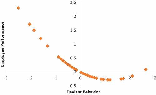
From the first equation, Figure 4 shows that a high innovation culture will reduce employees' desire to behave in a challenging manner. However, at the optimum point of -0.381, the desire for deviant behavior can increase with the assumption that the other variables are constant. Figure 5 also shows that the higher Deviant Behavior, the lower the Employee Performance.

Figure 4. The curve of the relationship between innovation culture and deviant behavior.

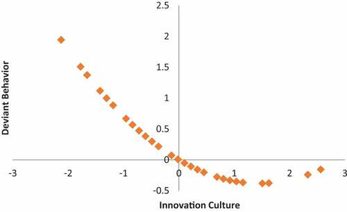
Figure 5. The curve of the relationship between innovation culture and employee performance.

12. Conclusions

The conclusions that can be delivered up to the second year research progress report are as follows:

1. Obtain a structural model that is robust with the assumptions of normality and homoscedasticity. Among them is the simple structural model theorem of efficient and consistent resampling approach; has produced complex structural model theorem with efficient and consistent resampling approach; has produced a simple structural model theorem with a weighted approach to solving the non-heteroscedasticity case; has produced the theorem of a complex structural model with a weighted approach to solving the non-heteroscedasticity case.

2. Obtain estimator properties from the flexible and robust SFAM structural model. Among them are the theorems of investigating the unbiased nature of simple structural models; have generated theorems investigating the unbiased nature of complex structural models; investigated the asymptotic nature of the simple structural model function obtained; have investigated the asymptotic nature of the function of the complex structural model obtained.

3. Obtaining hypothesis testing of each relationship built from the flexible and robust SFAM structural model. From the results of hypothesis testing, it was concluded that of the 18 institutions studied, seven agencies had a non-linear model, while 11 other agencies had a linear model.

Disclosure statement

No potential conflict of interest was reported by the author(s).

Additional information

Funding

The authors received no direct funding for this research.

References

- Asrun. (2014). Kepemimpinan spiritual: Pengaruhnya Terhadap Spiritualitas di Tempat Kerja, Kepuasan Kerja, dan Perilaku Menyimpang di Tempat Kerja. Disertasi, Universitas Brawijaya).
- Chen, H., & Wang, Y. (2011). A penalized spline approach to functional mixed effects model analysis. Biometrics, 67(1), 861–24. https://doi.org/10.1111/j.1541-0420.2010.01524.x
- Chin, W. W. (2006). Overview of the PLS Method.
- Dillon, W. R., & Goldstein, M. (1984). Multivariate analysis methods and applicationds. John Wiley dan Sons.
- Garson, G. D. (2013). Path analysis. Statistical Associates Publishing.
- Hair, J. F., Jr., Anderson, R. E., Tatham, R. L., & Black, W. C. (2010). Multivariate data analysis with reading. Macmillan Pub. Company.
- Handayanto. (2014) . Pengaruh Budaya Organisasi Terhadap Kepemimpinan, Nilai Personal, dan Perilaku Ihsan di Rumah Sakit Islam Masyitoh Bangil. Disertasi, Universitas Brawijaya).
- Heckman, N., Lockhart, R., & Nielsen, J. D. (2009). Penalized regression, mixed effects models and appropriate modelling. Retrieved, December, 12, 2012. Website: http://www.stat.ubc.ca/~nancy/pubs/lmetechreport.pdf
- Joreskog, K., & Sorbom, D. (1996). LISREL 8: User’s reference guide (Second Edition ed.). Scientific Software International, Inc.
- Fernandes, A. A. R. (2017). Investigation of instrument validity: Investigate the consistency between criterion and unidimensional in instrument validity (case study in management research). International journal of law and management.
- Fernandes, A. A. R. (2017). Moderating effects orientation and innovation strategy on the effect of uncertainty on the performance of business environment. International Journal of Law and Management.
- Fernandes, A. A. R., & Taba, I. M. (2018). Welding technology as the moderation variable in the relationships between government policy and quality of human resources and workforce competitiveness. Journal of Science and Technology Policy Management.
- Fernandes, A. A. R., Budiantara, I. N. I., Otok, B. W., & Suhartono. (2014). Reproducing Kernel Hilbert space for penalized regression multi-predictors: Case in longitudinal data. International Journal of Mathematical Analysis, 8(40), 1951–1961.
- Fernandes, A. A. R., Hutahayan, B., Arisoesilaningsih, E., Yanti, I., Astuti, A. B., & Amaliana, L. (2019, June). Comparison of curve estimation of the smoothing spline nonparametric function path based on PLS and PWLS in various levels of heteroscedasticity. In IOP Conference Series: Materials Science and Engineering (Vol. 546, No. 5, p. 052024). IOP Publishing.
- Fernandes, S., & Rinaldo, A. A. R. A. A. (2018). The mediating effect of service quality and organizational commitment on the effect of management process alignment on higher education performance in Makassar, Indonesia. Journal of Organizational Change Management.
- Purbawangsa, I. B. A., Solimun, S., Fernandes, A. A. R., & Rahayu, S. M. (2019). Corporate governance, corporate profitability toward corporate social responsibility disclosure and corporate value (comparative study in Indonesia, China and India stock exchange in 2013–2016). Social Responsibility Journal, 16(7), 983–999.
- Solimun. (2010). Analisis Multivariat Pemodelan Struktural. Citra.
- Sumardi, S., & Fernandes, A. A. R. (2020). The influence of quality management on organization performance: service quality and product characteristics as a medium. Property Management, 38(3), 383–403.
- Van der Seijs, M. V., de Klerk, D., & Rixen, D. J. (2016). General framework for transfer path analysis: History, theory and classification of techniques. Mechanical Systems and Signal Processing, 68, 217–244. https://doi.org/10.1016/j.ymssp.2015.08.004
- Verbekke, G., Fiews, S., Molenberghs, G., & Davidian, M. (2014). The analysis of multivariate longitudinal data: A review. Statistical Methods in Medical Research, 23(1), 42–59. https://doi.org/10.1177/0962280212445834
- Wiryatmojo, S. (2012). Pengaruh Kompetensi dan Motivasi Terhadap Intuisi dan Kinerja Aparat Reserse. Disertasi, Universitas Brawijaya).