A Bayesian model for online customer reviews data in tourism research: a robust analysis

Abstract

The Bayesian approach to data analysis is useful when the variables considered are already subjective or abstract, as is the case with online consumer reviews and ratings in tourism research. The Bayesian framework provides a method for combining observed data from prominent e-commerce platforms with other prior information, such as expert knowledge. Also, Bayesian statistical modelling has several advantages when the sample size of observed data is small. However, a source of uncertainty is introduced into the analysis by eliciting a unique prior distribution that adequately represents the expert’s judgement. We focus on the problem in a formal Bayesian robustness context by assuming that the hospitality manager is unable to choose a functional form for the prior distribution but that he or she may be able to restrict the possible priors to a class that is suitable for quantifying the practitioner’s uncertainty. Our interest is:

1. We propose a new distribution that is suitable for fitting the rating data.

2. We have shown how the practitioner can introduce his judgements about the feeling parameter using an appropriate prior distribution and

3. We develop a Bayesian robust methodology to manage hospitality managers’ uncertainty using a class of prior distributions suitable for quantifying the practitioner’s uncertainty.

These ideas were illustrated using real data. We demonstrate that the Bayesian robustness methodology proposed allows us to manage this uncertainty in our model by using classes of prior distributions and how the measures of interest are transformed into intervals of interest that will allow the manager to make decisions.

Keywords:

• Bayesian statistics
• online consumer reviews
• e-WOM
• statistical distribution
• Bayesian robustness

Reviewing Editor:

• Kaouther Kooli, Bournemouth University, United Kingdom of Great Britain and Northern Ireland

Subjects:

• Statistics & Probability
• Hospitality
• Tourism

1. Introduction

The request for customer comments through webpages is common for most companies, particularly those related to the hotel industry. In this sense, the collection of customer comments on pages such as Booking, TripAdvisor, Edreams, and Airbnb is well known.

According to the online booking website Expedia, customers are willing to pay 24% more for hotels with a rating of 3.9 vs. 2.4 (on a scale of 1 to 5) and 35% more for hotels with a 4.4 rating vs. 3.9. Therefore, companies collect reviews and ratings. Having consumers who experience the offer rate or review their business, ideally in a positive way, results in this information convincing other consumers to choose their establishment over others.

Platforms, apps, and other devices are now established channels for booking accommodation; therefore, customers and hotel managers need to understand travelers’ booking preferences and their propensity to book directly online (Peng et al., 2018). This knowledge can help both parties reduce costs (Lei et al., 2019). Single-value ratings are sometimes supplemented by multi-criteria ratings, text comments, and other resources (Chen et al., 2021; Nilashi et al., 2019; Zhao et al., 2019). Fong et al. (2017) used cognitive variables to predict tourists’ intention to use mobile apps to book hotels, while Boto-García et al. (2021) examined associations between trip characteristics, such as trip purpose, distance to origin, length of stay, and choice of booking mode, and found that different population groups have different preferences.

Many tourism and hospitality researchers have examined electronic word-of-mouth (eWOM) by examining data from major review sites, such as TripAdvisor (Fang et al., 2016) and Booking.com (Mellinas et al., 2015, 2016; Mellinas & Martin-Fuentes, 2021), while others have compared review sites (Xiang et al., 2017).

It is well known that the Bayesian approach to data analysis is particularly well-suited when the variables used are already subjective or abstract, such as in hospitality research in general and online consumer reviews or ratings. The Bayesian framework provides a method for combining observed data from prominent e-commerce platforms with other prior information such as expert knowledge. In addition, Bayesian statistical modelling has several advantages when the sample size of the observed data is small. In this study, we focus on the ratings and not on the reviews themselves reflected by the clients. Because the data indicate a subjective judgement, Bayesian statistics can be useful in this case (Bianchi & Heo, 2021). In Bayesian statistics, all uncertain quantities are modelled as probability distributions, and inferences are obtained through the posterior conditional probabilities for the unobserved variables of interest, given the observed data sample and prior assumptions, using Bayes’ theorem. However, a source of uncertainty is introduced into the analysis by eliciting a unique prior distribution that adequately represents an expert’s judgement. We focus on the problem in a formal Bayesian robustness context by assuming that the hospitality manager is unable to choose a functional form for the prior distribution, but that he or she may be able to restrict the possible priors to a class that is suitable for quantifying the practitioner’s uncertainty. Therefore, it is of interest to study how a relevant quantity, such as the (posterior) expected score, behaves in such a class.

Bayesian statistics have become more popular in business, economics, management, social sciences, and related fields owing to the increased processing power required to handle the complexity of statistical models. This approach has also helped the tourism management and hospitality disciplines, where Bayesian frameworks are more flexible and intuitive than frequentist frameworks (Assaf & Tsionas, 2019a).

Bayesian research on tourism and hospitality is still in its infancy. We highlight the works addressing cost efficiency and business efficiency estimated using Bayesian parametric and non-parametric stochastic frontier and DEA Bayesian approaches by Assaf (2009, 2011) and Assaf and Tsionas (2015, 2019b), efficiency in the US hotel industry (Assaf, 2012), regression and forecasting models (Assaf & Tsionas, 2019b), and Bayesian methods and structural equation modelling (Assaf et al., 2018), among others. Bianchi and Heo (2021) provide a good overview of Bayesian statistics in tourism management.

Similarly, there is little Bayesian research on eWOM in travel and hospitality, where frequentist methods are more common. Although focused on Bayesian clustering approach to managing score heterogeneity between OCR (online consumer review) websites, recently Martel-Escobar et al. (2023) also present a brief review of applications of Bayesian analysis in this area. In addition, Bianchi and Heo (2021) show how the Bayesian approach can improve hospitality management practices through its ability to deal with a lack of data, which is too often in the hotel industry, and incorporates experts’ opinions into quantitative analyses, allowing them to ‘measure the unmeasurable’, such as creativity, experience, fulfillment, or happiness. Bianchi and Heo (2021) established that, in microeconomic terms, reviews are related to customers’ utility and therefore play a role in customers’ decision-making processes. As a result, because decision analysis inputs contain the hotel manager’s judgment, they would be interested in determining the consequences and any inconsistencies in his/her judgements. The assessment of beliefs and preferences is a difficult task (even more so for several experts). Some argue that priors and utilities can never be quantified exactly, that is, without error, particularly in a finite amount of time. Within the Bayesian framework presented by Bianchi and Heo (2021), an elementary sensitivity analysis was developed to calculate the posterior quantities of interest (means and standard deviations) when several prior densities are considered.

In the literature on Bayesian tourism hospitality, only a few studies have examined the robustness of priors. Specifically, these papers are based on the study of a finite set of priors and then study the behavior of certain quantities of interest in this catalogue of distributions. Bianchi and Heo (2021) showed the range of the (posterior) expected score when the elicited prior mean ranged from 10 to 6 (i.e. five gamma prior distributions were considered). Comerio and Pacicco (2021) conducted a Bayesian VAR to analyze the economic impact of tourism in Japanese prefectures and report the effect of priors on two VAR(1) and two AR(1) models. Assaf and Tsionas (2021), using an artificial simulated dataset in a regression context, show the behavior of the Bayes factor for hypothesis testing for three different priors on the following parameters: a conjugated normal model with a non-informative prior on the variance, a joint non-informative model, and the Jeffreys-Zellner–Siow priors for linear regression (Zellner & Siow, 1980). Finally, Assaf and Tsionas (2018) also used a Bayesian VAR model to measure hotel performance with respect to productivity and efficiency with a dataset of 613 hotels located across the US, Europe, the Middle East, and the Asia Pacific for the period 2012–2016. An intensive sensitivity study was developed generating 10000 random prior parameters and compute the associated values of the new posterior means and standard deviations to make comparisons with the baseline posterior mean and standard deviation obtained for the elicited base prior. Robust behavior of the quantities of interest was observed. As the authors mentioned, ‘these results indicate that prior sensitivity is not an important issue in this study, so we can proceed with reporting results from our baseline prior specification’. However, a robust Bayesian approach can be proposed and used to improve the empirical approach.

In Bayesian analysis, choosing a prior distribution based on prior knowledge and preferences is a difficult task. In practice, the practitioner or decision-maker usually chooses convenient approximations of the subjective prior. The legitimacy of such an approximation can be investigated by a sensitivity (robustness) analysis of the results with respect to the approximations. This is the purpose of robust Bayesian analysis (see for instance, Berger, 1985 and Ríos & Ruggeri, 2000; among others). An interesting approach, called global robustness, which will be used here, proposes replacing a single prior distribution by a class of priors and then computing the range of the ensuing answers as the prior varies over the class.

Our approach is based on the assumption that the hospitality manager is unable to choose a functional form for the prior distribution but that he or she may be able to restrict the possible priors to a class that is suitable for quantifying the practitioner’s uncertainty. Therefore, it is of interest to study how a relevant quantity, such as the (posterior) expected score, behaves in such a class. That is, Bayesian robustness analysis provides an interval of variation for the expected score. We obtain the upper and lower bounds of these intervals by solving complex mathematical programming problems, including techniques of variational programming. Fortunately, this work simplifies the variational problems by focusing on finding the extremes of one variable’s functions, which we can then solve numerically to obtain the explicit solutions of the upper and lower bounds. Technical details are shown in the appendix.

The remainder of this paper is organized as follows. Section 2 discusses the proposed sampling model and standard Bayesian approach for inference purposes. In Section 3, the Bayesian robustness of the average rating parameter is addressed rigorously. We address this problem by replacing a unique prior distribution (as required by standard Bayesian analysis) with a complete class of prior distributions that are compatible with the expert’s judgements. Section 4 presents an empirical data illustration based on the two datasets. Finally, concluding remarks are presented in Section 5. The proofs and technical details are provided in the Appendix.

2. A rescaled shifted binomial model for customers’ reviews

The rating information comprises summaries of how much a product was liked by reviewers (for example, on a discrete scale ranging from 1 to 10 on the Booking platform), the number of people who rated the product, and the average rating of all reviews.

Concerns about the amount of individual ratings used to produce an average value may arise when reviewing online consumer evaluations; clearly, average ratings based on numerous perspectives are more robust information sources than those based on only a few (Hoffart et al., 2019). As a result, researchers want to know how the parameter that represents the average rating $\theta$, behaves in order to obtain a fair estimate of the expected score.

Bianchi and Heo (2021) assume that the number of customer reviews, online customer review ratings for hotels, and the probability that a score $X$ is equal to $x$, follows a Poisson distribution with mean $\theta$>0 defined on a parameter space $\mathrm{\Theta }$, that is, $$\mathrm{\text{Pr}}\left(\mathrm{X}=\mathrm{x}\right)=\mathrm{\text{exp}}\hspace{0.17em}\left(-\theta \right)\frac{{\theta }^x}{x!},x=0,1,\dots$$

However, the Poisson distribution does not seem adequate to model the variable of interest for two reasons: (i) the support of variable $X$ is bounded between 1 and 10, and (ii) empirical data of this nature are underdispersed (variance lower than the mean). It is well known that the Poisson distribution shows equidispersion, that is, the mean and variance are equal.

D’Elia and Piccolo (2005) addressed the problem of modeling and analyzing preference data, specifically ranking data, by proposing a mixture of uniform and shifted binomial distributions called the MUB model. The MUB model aims to capture uncertainty and heterogeneity in the elicitation process of preferences. Recently, Li and Chen (2023) proposed a new model for rating data, in which some customers were reluctant to assign the lowest score to a product. This study suggests that a two-component shifted binomial mixture (SBM) model is a better choice for many rating datasets.

For this reason, we provide a more reliable model based on binomial distribution. Thus, we assume that the probability that a score X is equal to x follows a rescaled shifted binomial distribution with mean $\theta$>0 defined on a parameter space $\mathrm{\Theta }=(1,\mathrm{m}+1)$ and with a probability mass function given by (1) $$\text{Pr}\left(X=x\right)=\left(\begin{array}{c}m\\ x-1\end{array}\right){\left(\frac{\theta -1}{m}\right)}^{x-1}{\left(1-\frac{\theta -1}{m}\right)}^{m-x+1},x=1,2,\dots ,m+1$$(1) where $1<\theta <m+1$ and $m>0.$

The mean and variance of this distribution are given by, $$\mathbb{E}\left(X\right|\theta )=\theta ,$$ $$\mathit{\text{var}}(X\theta )=\left(\theta -1\right)\left(1-\frac{\theta -1}{m}\right),$$ respectively. Since the index of dispersion of this distribution is given by $$\text{ID}=\frac{\text{var}\left(X\right)}{E\left(X\right)}=1-\left(\frac{{\left(\theta -1\right)}^2}{\text{m\hspace{0.17em}\hspace{0.17em}\hspace{0.17em}}\theta }\right)-\frac{1}{\theta }<1$$ it follows that the distribution is underdispersed ($\mathit{\text{var}}\left(X\right)<\mathbb{E}(X))$ for all values $m$ and $\theta$.

In practice, the integer $m$ is assumed to be known ($m=9$ in our case); therefore, the focus is on the parameter $\theta$, that is, the mean of the rescaled shifted binomial population rating data. As Bianchi and Heo (2021) point out, what are our expectation concerning the mean parameter?

Parameter $\theta$ also controls the degree of skewness of the rating data distribution, and is referred to as the feeling parameter (Simone, 2021). Its meaning can be changed depending on what is being studied so that $\theta$ can be used as a measure of happiness, trust, risk perception, etc. Depending on how the scale is written and how it is oriented, the results can be expressed in terms of $1-\theta$ instead of $\theta$. For example, if higher scores on the scale indicate stronger feelings, then $1-\theta$ is a direct indicator of the latent concept.

Every discrete ordinal choice has an underlying degree of uncertainty caused by indecision in the response. Keeping this in mind, the inclusion of the hospitality managers’ expert judgement in our statistical analysis is appropriate, and the Bayesian perspective follows naturally. Under Bayesian methodology, expert opinions must be considered as a probability distribution (called prior distribution) that adequately represents these opinions. This prior distribution represents the distribution of the values of $\theta$ across the population of potential customers.

Now, assuming that rater $i$ rates a given hotel according to a distribution with pmf given in (1) and makes rates independent across raters, the likelihood for the data is (2) $$L\left(\theta \right)=\prod _{i=1}^n\mathrm{\text{Pr}}\left(X_i=x_i\right)\propto {\left(\theta -1\right)}^{x^{+}-n}{\left(m+1-\theta \right)}^{n\left(m+1\right)-x^{+}},$$(2) where $x^{+}={\sum }_{i=1}^n{x}_i$, $n$ is the sample size, and symbol $\propto$ means ‘proportional to’.

2.1. The Bayesian perspective

We now assume that the parameter $\theta$ is allowed to vary between customers with a prior distribution and a probability density function (pdf) given by (3) $${\pi }_0\left(\theta \right)=\frac{{\left(\theta -1\right)}^{\alpha -1}{(m+1-\theta )}^{\beta -1}}{m^{\alpha +\beta -1}B(\alpha ,\beta )},1<\theta <m+1,$$(3) which is the classical beta distribution, but with conveniently altered location and scale¹. Here, $B\left(\alpha ,\beta \right)={\int }_0^1{t}^{\alpha -1}{(1-t)}^{\beta -1}\mathit{\text{dt}}$ is the beta function.

As usual, this prior distribution represents our uncertainty about the true value of the parameter of interest $\theta .$

The mean, variance, and mode of this prior distribution are given by $$\mathbb{E}\left(\theta \right)=\frac{\alpha \left(m+1\right)+\beta }{\alpha +\beta },$$ $$\mathit{\text{var}}\left(\theta \right)=\frac{m^2\alpha \beta }{(\alpha +\beta +1{\left)\right(\alpha +\beta )}^2},$$ $${\theta }_0=\frac{\left(\alpha -1\right)\left(m+1\right)+\beta -1}{\alpha +\beta -2},\hspace{0.17em}\alpha >1,\beta >1,$$ respectively.

Given the sample $\tilde{x}=(x_1,\dots ,x_n)$, the expert judgements about $\theta$ are now updated through the Bayes’ theorem, and a posterior distribution can be obtained as follows: $$\pi (\theta \tilde{x})=\frac{{\pi }_0\left(\theta \right)L\left(\theta \right)}{m\left(\tilde{x}\right)}\propto L\left(\theta \right){\pi }_0\left(\theta \right).$$

That is, the posterior distribution $\pi (\theta |\tilde{x})$ is proportional to the product of the likelihood $L\left(\theta \right)$ and the prior distribution ${\pi }_0\left(\theta \right)$. Here, $m\left(\tilde{x}\right)={{\displaystyle \int }}_{\Theta }L\left(\theta \right){\pi }_0\left(\theta \right)d\theta$ is a constant that depends only on the observed sample data $\tilde{x}$ and does not depend on $\mathrm{\theta }$ and the parameter space $\mathrm{\Theta }$ is given by the interval $\left(1,m+1\right)$.

Therefore, from (2(2) $$L\left(\theta \right)=\prod _{i=1}^n\mathrm{\text{Pr}}\left(X_i=x_i\right)\propto {\left(\theta -1\right)}^{x^{+}-n}{\left(m+1-\theta \right)}^{n\left(m+1\right)-x^{+}},$$(2) ) and (3(3) $${\pi }_0\left(\theta \right)=\frac{{\left(\theta -1\right)}^{\alpha -1}{(m+1-\theta )}^{\beta -1}}{m^{\alpha +\beta -1}B(\alpha ,\beta )},1<\theta <m+1,$$(3) ), the posterior distribution of parameter $\mathrm{\theta }$ is again a shifted beta distribution with location and scale altered as in (2(2) $$L\left(\theta \right)=\prod _{i=1}^n\mathrm{\text{Pr}}\left(X_i=x_i\right)\propto {\left(\theta -1\right)}^{x^{+}-n}{\left(m+1-\theta \right)}^{n\left(m+1\right)-x^{+}},$$(2) ), given by $${\alpha }^{\text{*}}=\alpha +x^{+}-n,$$ $${\beta }^{\text{*}}=\beta +n\left(m-1\right)-x^{+}.$$

Thus, the posterior mean and variance of the parameter $\theta$ are given by, (4) $${\rho }^{{\pi }_0}\left(\tilde{x}\right)=\frac{{\alpha }^{\text{*}}\left(m+1\right)+{\beta }^{\text{*}}}{{\alpha }^{\text{*}}+{\beta }^{\text{*}}}=\frac{\text{α}\left(m+1\right)+\beta +m{x}^{+}}{\text{α}+\beta +\mathit{\text{nm}}},$$(4) (5) $$\mathit{\text{va}}{r}^{{\pi }_0}\left(\tilde{x}\right)=\frac{m^2{\alpha }^{\text{*}}{\beta }^{\text{*}}}{\left({\alpha }^{\text{*}}+{\beta }^{\text{*}}+1\right){\left({\alpha }^{\text{*}}+{\beta }^{\text{*}}\right)}^2},$$(5) respectively.

There are advantages to using a conjugate prior (the posterior is in the same form as the prior for the likelihood considered) because it simplifies the computations and provides a good interpretation of the posterior. Observe that (4(4) $${\rho }^{{\pi }_0}\left(\tilde{x}\right)=\frac{{\alpha }^{\text{*}}\left(m+1\right)+{\beta }^{\text{*}}}{{\alpha }^{\text{*}}+{\beta }^{\text{*}}}=\frac{\text{α}\left(m+1\right)+\beta +m{x}^{+}}{\text{α}+\beta +\mathit{\text{nm}}},$$(4) ) can be written as: (6) $${\rho }^{{\pi }_0}\left(\tilde{x}\right)=\frac{\mathit{\text{nm}}}{\alpha +\beta +\mathit{\text{nm}}}\overline{x}+\frac{\alpha +\beta }{\alpha +\beta +\mathit{\text{nm}}}\mathbb{E}\left(\theta \right),$$(6) where $\overline{x}=x^{+}/n$ denotes the sample mean. That is, we see that the posterior expectation is a weighted average of the sample mean $\overline{x}\mathrm{ }$ and prior expectation $\mathbb{E}\left(\mathrm{\theta }\right).$ Thus, (7) $${\rho }^{{\pi }_0}\left(\tilde{x}\right)=\gamma \left(n\right)\overline{x}+\left(1-\gamma \left(n\right)\right)\mathbb{E}\left(\theta \right),$$(7) where the weighted factor $\mathrm{\gamma }\left(n\right)=\mathit{\text{nm}}/\left(\alpha +\beta +\mathit{\text{nm}}\right)\in \left[0,1\right]$ is given by (8) $$\gamma \left(n\right)=\frac{n\mathit{\text{var}}\left[{\mathbb{E}}_{\theta }(X\theta )\right]}{n\mathit{\text{var}}\left[{\mathbb{E}}_{\theta }(X\theta )\left]+\mathbb{E}\right[\mathit{\text{va}}{r}_{\theta }(X\theta )\right]}.$$(8)

If the sample size is large, then $\overline{x}$ is a reliable estimate of $\mathrm{\theta }$. The estimator ${\rho }^{{\pi }_0}\left(\tilde{x}\right)$ takes advantage of this by assigning its weights on $\overline{x}\mathrm{ }$ and $\mathbb{E}\left(\mathrm{\theta }\right)$ to one and zero, respectively, as the sample size increases. Furthermore, the statistical properties of $\overline{x}\mathrm{ }$ and $\mathbb{E}\left(\mathrm{\theta }\right)$ are essentially the same for large sample sizes. That is, from (6) it can be seen that as $n\mathrm{ }$ goes to infinity, the posterior mean coincides with the sample mean. Then, the best estimators of parameter $\mathrm{\theta }$ are obtained using classical (non-Bayesian) statistics. When little data are available, that is, $n\mathrm{ }$ for example, goes to zero, the best estimator of $\mathrm{\theta }$ is the prior mean $\mathbb{E}\left(\mathrm{\theta }\right)$. Here is one advantage of using Bayesian statistics is that little data are available. In conclusion, the quantity ${\rho }^{{\pi }_0}\left(\tilde{x}\right)$ allows us to combine data with prior information to stabilize our estimation of $\mathrm{\theta }$.

In (8), $\mathit{\text{var}}\left[{\mathbb{E}}_{\theta }\left(X\right|\theta )\right]$ is a measure of the heterogeneity of the customer population, while $\mathbb{E}\left[{\mathit{\text{var}}}_{\theta }\left(X\right|\theta )\right]$ provides a global measure of the dispersion of these means among all customers in this population. This occurs for all conjugate families of the distribution under the sampling exponential family of distribution. For example, see Diaconis and Ylvisaker (1979). As Lee (1997, p. 63) points out, the family of conjugate priors is large enough that there is one that is sufficiently close to your real prior belief that the resulting posterior is barely distinguishable from the posterior that comes from using your real prior. For additional properties of this posterior mean, refer to Ericson (1969). As a conspicuous reviewer pointed out, rating data may have characteristics for which Lee’s statement doesn’t apply (for instance, two groups of raters: one who loves the hotel and one who is very disappointed; that is, a bimodal situation is present). Fortunately, Chang et al. (2020) empirically found that for luxury hotels, the average hotel scores presented a left-skewed distribution with a unique mode, whereas a conjugated prior distribution of the exponential family seems appropriate.

The advent of Markov Chain Monte Carlo (MCMC) techniques has led to an increase in the popularity of the Bayesian methodology even when likelihood function and priori distributions doesn’t present the conjugancy property. By using these simulation-based methods, we may solve problems based on extremely complicated models numerically. Unfortunately, sensitivity analysis in MCMC techniques is a difficult task and constitutes a challenging undertaking today, as presented in Pérez et al. (2006). As we will see in the next section, this fact can be circumvented by using conjugate distributions without the need to introduce additional mathematical complexities. In this context, we prefer a conjugate model.

3. Robustness of the posterior feedback

The values of (4(4) $${\rho }^{{\pi }_0}\left(\tilde{x}\right)=\frac{{\alpha }^{\text{*}}\left(m+1\right)+{\beta }^{\text{*}}}{{\alpha }^{\text{*}}+{\beta }^{\text{*}}}=\frac{\text{α}\left(m+1\right)+\beta +m{x}^{+}}{\text{α}+\beta +\mathit{\text{nm}}},$$(4) , 9(9) $${\mathrm{\Gamma }}^{\mathrm{\epsilon }}=\left\{\mathrm{\pi }\left(\mathrm{\theta }\right)=\left(1‐\mathrm{\epsilon }\right){\mathrm{\pi }}_0\left(\mathrm{\theta }\right)+\mathrm{\epsilon }q\left(\mathrm{\theta }\right),q\in \mathrm{\Gamma }\right\},$$(9) , 10(10) $$\Gamma =\left\{\text{all unimodal probability distributions with the same mode,}{\theta }_0,\text{as that of\hspace{0.17em}}{\pi }_0\right\}.$$(10) ), and (5(5) $$\mathit{\text{va}}{r}^{{\pi }_0}\left(\tilde{x}\right)=\frac{m^2{\alpha }^{\text{*}}{\beta }^{\text{*}}}{\left({\alpha }^{\text{*}}+{\beta }^{\text{*}}+1\right){\left({\alpha }^{\text{*}}+{\beta }^{\text{*}}\right)}^2},$$(5) ) depend on the selection of parameters of the prior distribution. In practice, we assume that practitioners are unable to specify a simple prior distribution for the expected score. The practitioner or decision-maker typically chooses convenient approximations to the subjective prior. We can examine the validity of this approach by conducting a sensitivity analysis of the results in relation to the approximations. We then compute the range of the resulting answers by varying the prior judgments within this set.

3.1. Formalizing the idea of robustness

Robust Bayesian analysis is based on the idea that the prior belongs to a family of possible distributions instead of a single distribution. According to the robust Bayesian methodology, uncertainty in the prior can be modelled by specifying a class of priors instead of a single one. Thus, we examine the ranges of customer review ratings when priors belong to such a class. The most robust Bayesian procedures have led to sensitivity measures of quantities that can be expressed in terms of posterior expectations (e.g. the mean, variance, and probability of sets). We evaluate the robustness of ${\rho }^{\mathit{\pi }}\left(\tilde{x}\right)$ by considering the interval $$\left(\underset{\_}{\rho },\overline{\rho }\right)\text{\hspace{1em}where\hspace{1em}}\underset{\_}{\rho }=\underset{\pi \hspace{0.17em}\in \hspace{0.17em}\Gamma }{\mathit{\text{inf}}}{\rho }^{\pi }\left(\tilde{x}\right),\overline{\rho }=\underset{\pi \hspace{0.17em}\in \hspace{0.17em}\Gamma }{\mathit{\text{sup}}}{\rho }^{\pi }\left(\tilde{x}\right),$$

That is, $\mathrm{ }\underset{¯}{\mathrm{\rho }}$ and $\overline{\mathrm{\rho }}$ are the lower and upper bounds, respectively, of the quantity of interest ${\rho }^{\pi }\left(\tilde{x}\right)$ over the class of priors $\mathrm{\Gamma }.$

The problem discussed in this study has two additional characteristics. On the one hand, the measure by which the sensitivity is evaluated is determined by the same structure of the problem, which in this case is the point estimates of the average score $\mathrm{\theta }.$ Furthermore, the a priori class of feasible distributions must be defensible and familiar to the hospitality manager.

We will test the sensitivity of the posterior mean by including a measure whose magnitudes do not depend on the measurement units of the quantity of interest. This is the factor of relative sensitivity RS introduced by Sivaganesan (1991), and is given by $$\mathit{\text{RS}}=\frac{\overline{\rho }-\underset{\_}{\rho }}{2{\rho }^{{\pi }_0}\left(\tilde{x}\right)}\times 100\text{\%}$$

Factor RS has an intuitive meaning and can be thought of as the percentage variation of the average score around a specific base prior as the prior varies in class $\Gamma .$ A modest value of RS indicates robustness with respect to a specific benchmark prior, and the hotel managers will have few questions about the average score obtained from the ‘true’ base prior. A large value of RS, on the other hand, indicates that the prior needs to be refined further. In the context of meta-analysis of medical treatment data and with different classes of prior distributions, an application of the robust Bayesian methodology using the RS factor can be found in Vázquez et al. (2016).

This study was carried out using the $\mathrm{\epsilon }$-contaminated classes (Berger, 1985; Ríos & Ruggeri, 2000; Gómez-Déniz et al., 2000; among others). If ${\pi }_0$ is the base-elicited prior, the $\mathrm{\epsilon }$-contaminated class is given by (9) $${\mathrm{\Gamma }}^{\mathrm{\epsilon }}=\left\{\mathrm{\pi }\left(\mathrm{\theta }\right)=\left(1‐\mathrm{\epsilon }\right){\mathrm{\pi }}_0\left(\mathrm{\theta }\right)+\mathrm{\epsilon }q\left(\mathrm{\theta }\right),q\in \mathrm{\Gamma }\right\},$$(9) where ${\pi }_0\left(\theta \right)$ is a base prior that would be used in a single prior Bayesian analysis with limited confidence, derived from past experience, control studies, and/or subjective judgment. The parameter $\epsilon \in \left[0,1\right]$ is the amount of contamination that indicates the degree of ambiguity about the benchmark prior ${\pi }_0\left(\theta \right)$ and $\mathrm{\Gamma }$ is a class of contamination distributions spanning plausible priors.

Recently, Chang et al. (2020) empirically found that for luxury hotels, the average hotel scores presented a left-skewed distribution with a unique mode where a conjugated shifted beta base prior distribution seems appropriate. Therefore, we look for classes of prior distributions in which the shape preferences for the prior distributions might be expressed. In particular, given that the mode is a very intuitive statistical concept, hotel managers with good daily training in revising online customer reviews should not have any problem in assessing the unimodality of the average score parameter and its numerical value.

A natural choice is then the unimodality assumption, and thus taking the class, (10) $$\Gamma =\left\{\text{all unimodal probability distributions with the same mode,}{\theta }_0,\text{as that of\hspace{0.17em}}{\pi }_0\right\}.$$(10)

Furthermore, this class has several interesting features. It is simple to elicit, contains as many plausible prior distributions as feasible, and is simple to employ in numerical computations, as suggested by Berger (1985).

Expressions for the lower and upper bounds for ${\rho }^{\mathit{\pi }}\left(\tilde{x}\right)$ can be found in Appendix. In the following section, we illustrate this proposed methodology with real data. Dataset 1 (Gstaad Palace Hotel) was retrieved from Booking.com on January 23, 2023 (at 12:50 CET). Dataset 2 (Bellevire Gstaad Hotel) was extracted from Booking.com on February 4, 2023, at 17:06 p.m. CET. All data was sourced from the publicly available Booking.com platform and has already been published; no further permission is required for its utilization for research purposes.

4. Data and results

To illustrate the preceding developments, we present an analysis of two real datasets. First, following Bianchi and Heo (2021), we analyze customers’ online reviews from the Gstaad Palace (dataset number 1), a well-known five-star hotel located in the Swiss Alps. We retrieved ratings from Booking.com on January 23, 2023 (at 12:50 CET). This dataset contains $n=120$ ratings observations, ranging from 1 (indicating a ‘very poor’ experience) to 10 (a ‘superb experience, i.e. $m=9$). Given the luxury category of the considered hotel, we expect a skewed left rating distribution (in fact, 98 of the observed ratings for this hotel correspond to a maximum score of 10).

Analogously, dataset 2 contains $n=471$ rating observations from the Bellevire Gstaad Hotel, a three-star hotel managed by the same firm and next to the previous one (data extracted from Booking.com, on February 04, 2023, at 17:06 pm CET). In this case, only 136 of the 421 observed scores had the highest rating.

As Table 1 and Figure 1 show, we have data with clearly low dispersion. In addition, the Gstaad Hotel dataset corresponds to a very strongly skewed left distribution (i.e. a very high customer satisfaction rating or what in statistical terms is equivalent to a very high value for the most frequent score value, that is, its mode). In addition, the Bellevire Gstaad Hotel dataset presents a score distribution with a lower mode value, and thus a distribution that is not so strongly skewed to the left.

Figure 1. Histograms of the rating data sets: Gstaad Palace Hotel (left figure) and Bellevire Gstaad Hotel (right figure).

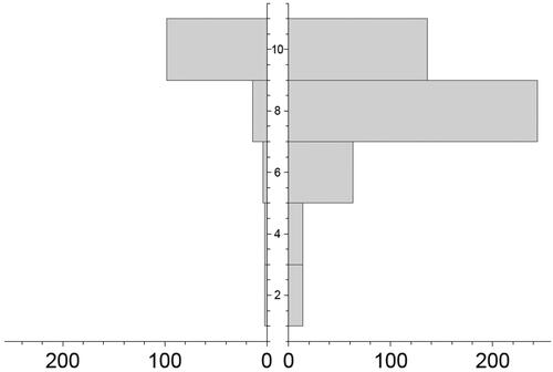
Table 1. Customer score distribution for the two data sets considered.

	Data set #1 (Gstaad palace hotel)	Dataset #2 (Bellevire Gstaad hotel)
Score	Frequency	Frequency
[1,3)	2	14
[3,5)	2	14
[5,7)	4	63
[7,9)	14	244
[9,10]	98	136
Total	120	471
Descriptive summaries
Average score	9.40	8.01
Standard Deviation	1.52	1.80
Index of Dispersion	0.25	0.40

4.1. Fitting data distribution

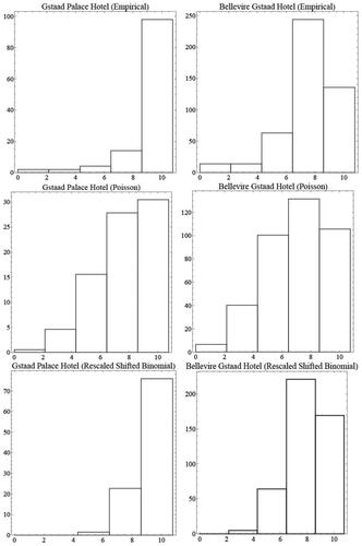
The sample dispersion index of the datasets 0.25 and 0.40, respectively, are markedly lower than 1, indicating that there is underdispersion. For illustrative purposes, Table 2 shows the fits from the Poisson model and the proposed rescaled shifted binomial models to the data sets.

Table 2. Maximum likelihood estimate $\widehat{\mathrm{\theta }},$ standard error (SE) of $\widehat{\mathrm{\theta }}$ and AIC value for the both data sets and sampling distributions considered.

	Dataset #1			Dataset #2
Fitted distribution	$\widehat{\mathrm{\theta }}$	SE	AIC	$\widehat{\mathrm{\theta }}$	SE	AIC
Poisson	9.4	0.280	528.472	8.013	0.130	2063.190
Rescaled shifted binomial	9.4	0.106	399.256	8.013	0.057	1934.050

The Akaike Information Criterion (AIC) is used to compare the estimated models. It is well known that a model with the minimum AIC value is preferred.

The estimation of the parameter $\mathrm{\theta }$ by the maximum likelihood method is presented in Table 2.

Given a sample $\tilde{x}=\left(x_1,\dots ,x_n\right)$ for the Poisson model it is well known that the maximum likelihood estimate of the mean parameter $\mathrm{\theta }$ is given by the sample mean $\widehat{\mathrm{\theta }}=\overline{x}=x^{+}/n$.

However, for the rescaled shifted binomial model, the maximum likelihood estimator of parameter $\mathrm{\theta }$ is obtained as the nontrivial root of the log-likelihood equation provided by differentiating in (2(2) $$L\left(\theta \right)=\prod _{i=1}^n\mathrm{\text{Pr}}\left(X_i=x_i\right)\propto {\left(\theta -1\right)}^{x^{+}-n}{\left(m+1-\theta \right)}^{n\left(m+1\right)-x^{+}},$$(2) ). After some algebra, the maximum likelihood estimates are also given by the sample mean $\widehat{\mathrm{\theta }}=\overline{x}=x^{+}/n$. The standard error is given by $$\sqrt{\mathrm{v}\mathrm{\text{ar}}\left(\widehat{\mathrm{\theta }}\right)}={\left[\text{n m}/\left(\left(\widehat{\mathrm{\theta }}-1\right)\left(\mathrm{m}+\widehat{\mathrm{\theta }}-1\right)\right)\right]}^{-1/2}.$$

Table 2 shows that, based on the AIC, the rescaled shifted binomial distribution model performs very well in fitting the distribution. Moreover, as Figure 2 shows, our proposal captures more adequately the rating classes where the highest frequency is observed, that is, the score interval [9,10] in the dataset #1 and $[7,9)$ in the dataset #2. These are the rating classes most visited by customers and where the Poisson model has very poor fits.

Figure 2. Top to down: Empirical and fitted frequencies of the two models considered (Poisson and rescaled shifted binomial distributions) of customers’ review data. Dataset #1 left and dataset #2 right.

4.2. The prior distribution

For illustrative purposes, in this section, we will show a simple way to incorporate hospitality manager experts’ judgements about the feeling parameter $\mathrm{\theta }$ into statistical modelling. The application of Bayes’ theorem involves a combination of the prior information of $\mathrm{\theta }$ with the likelihood of rating data observations. The result of this combination is a posterior distribution from which any probability statement can be generated. It is difficult to choose a prior distribution for an hospitality data analysis because it depends on the situation and goal of the analysis. However, there are some things to look for and ways to do things that can help guide this process. Coherence is important because the prior distribution should match the reasoning and structure of the model and the parameter space. Also, conjugacy should be taken into account, as the prior distribution should be mathematically compatible with the likelihood function. Data compatibility is also important because the prior distribution should match the data and should not contradict or overpower the evidence (Stefan et al., 2022). Winkler (1968) shows that it is possible to ask people about their subjective prior probability distributions, but this depends on the observer and the method(s) used to do so.

In the problem of eliciting a parametric prior distribution, the relationship between their hyperparameters and the usual descriptive measures such as mean and mode are frequently present; thus, the elicitation process reduces to the task of determining hyperparameter values that correspond to their expressed views (O’Hagan et al., 2006, chapter 6). If certain quantities, such as the mean and/or mode, require the focus of the elicitation, direct elicitation may be employed. This strategy can be implemented relatively quickly and easily if the expert is comfortable conveying their opinions on the quantity of interest. Although statistical training of hospitality managers should not be great, such descriptive measures are strongly intuitive and do not require more than a certain degree of experience for coherent elicitation.

For instance, in the case of the Gstaad Palace Hotel (dataset #1), suppose that the hospitality manager a priori assumes that $\mathbb{E}\left(\Theta \right)=9$ (roughly speaking, the manager can expect a total of scores of 45 for every $n=5$ ratings observations, which is in concordance with the observed sample data and the corresponding luxury category of the hotel). In order to show how our robust methodology, developed in the previous section, works, we present an elicitation experiment for a baseline prior distribution ${\pi }_0\left(\theta \right)$ in two scenarios: the Poisson sampling model, and our proposed rescaled shifted binomial sampling model. Thus, a base conjugated gamma prior is required in the Poisson case and a conjugated shifted beta prior in the second case.

As Watson and Moritz (2000) shows, researchers who wish to use expert knowledge may have difficulty distinguishing between quantities such as mean and mode, possibly because they tend to assume symmetrical (Gaussian) behaviors in the prior distribution, a situation that does not occur in this case, given the asymmetric profile of the gamma and the shifted beta for which we conduct an elicitation. Consequently, we consider that the manager suggests that the most frequent value for $\mathrm{\theta }$ is approximately 9, that is, $\mathrm{\theta }\approx 9.$

Therefore, for the Poisson sampling model, we observe that a gamma prior with shape parameter $\mathrm{\alpha }$ and scale parameter $\mathrm{\beta }$ verifies $\mathbb{E}\left(\Theta \right)=\mathrm{\alpha }/\mathrm{\beta }\mathrm{ }$ and $\mathit{\text{Mo}}\left(\Theta \right)=\left(\alpha -1\right)/\mathrm{\beta }.$ Hence, equating these quantities with elicited values provides a direct gamma prior distribution that is coherent with expert knowledge. Analogously, we proceed with the elicitation of a shifted beta distribution, considering the expressions of mean and mode (a priori) given in (3(3) $${\pi }_0\left(\theta \right)=\frac{{\left(\theta -1\right)}^{\alpha -1}{(m+1-\theta )}^{\beta -1}}{m^{\alpha +\beta -1}B(\alpha ,\beta )},1<\theta <m+1,$$(3) ).

Table 3 lists the prior values of the hyperparameters obtained from the aforementioned scenarios. As mentioned above, expert judgements in Table 3 should be understood as values that are assigned by the expert, but that the expert is not able to differentiate from other close value. For instance, in the case of Poisson-gamma and dataset #2, the elicited prior parameters $\mathrm{\alpha }$ and $\mathrm{\beta }$ values obtained from a mean and mode close to the value $8$ are $62.7$ and $7.84$ With these values, the (a priori) mean and mode of a gamma distribution are $7.99$ and 7.87, respectively. We assume that both values are indistinguishable from $8$ for a hospitality manager.

Table 3. Elicitation of prior distributions: expert’s judgements, corresponding hyperparameters values and posterior quantities.

Poisson-gamma
	Expert judgement		Elicited prior parameters		Sample data		Posterior quantities
Hotel	Mean	Mode	$\mathrm{\alpha }$	$\mathrm{\beta }$	$n$	$x^{+}$	${\alpha }^{\mathrm{*}}$	${\beta }^{\mathrm{*}}$	${\rho }^{{\pi }_0}\left(\tilde{x}\right)$
Gstaad	9	9	180	20	5	46	226	25	9.04
					10	82	262	30	8.74
Bellevire G.	8	8	62.7	7.84	5	44	106.70	12.84	8.31
					10	96	158.70	17.84	8.89
Rescaled shifted binomial-shifted beta
	Expert Judgement		Elicited prior parameters		Sample data		Posterior quantities
Hotel	Mean	Mode	$\mathrm{\alpha }$	$\mathrm{\beta }$	$n$	$x^{+}$	${\alpha }^{\mathrm{*}}$	${\beta }^{\mathrm{*}}$	${\rho }^{{\pi }_0}\left(\tilde{x}\right)$
Gstaad	9	9	15	2	5	46	56	6	9.13
					10	82	87	20	8.32
Bellevire G.	8	8	10	3	5	44	49	9	8.60
					10	96	96	7	9.39

A similar reasoning applies to the Gstaad Hotel (dataset #1), where the a priori estimate of the emotion parameter $\mathrm{\alpha }$ is approximately $9.$ For instance, the elicited prior values of $\alpha =15$ and $\mathrm{ }\beta =2$ in the rescaled shifted binomial-shifted beta provide mean and mode (a priori) values of $8.94$ and $9.4$, respectively, which can be considered indistinguishable from $9.$

Table 3 also contains the Bayesian estimation of the feeling parameter $\mathrm{\theta }$ given by the posterior mean ${\rho }^{\pi }0\left(\tilde{x}\right)$ for all settings considered. In addition, we simulate two practical situations with small sample sizes, as in the case of a hospitality manager who updates his judgements only with the most recent online ratings. We have assumed the cases of the sample size $n$ equal to $5\mathrm{ }$ and $10,$ with cumulative ratings of $46$ and $82$ in the case of Gstaad Hotel, and $44$ and $96$ in the case of Bellevire Gstaad Hotel, respectively.

4.3. Robustness of the customers’ review

As mentioned in Section 2, the rating information includes summaries of the extent to which reviewers enjoyed a product (scored on a discrete scale ranging from the lowest to the highest possible rating), the number of individuals who have evaluated the product, and the average rating of all reviews. Evidently, average ratings based on many opinions are more robust information sources than those based on only a few (Hoffart et al., 2019). Therefore, researchers wish to determine the behavior of the parameter that represents the average ratings $\mathrm{\theta },$ to obtain an expected score for the customers’ review.

However, the practitioner may be unable to provide appropriate information on a uniquely determined prior of $\mathrm{\theta }$ probably because of insufficient knowledge to identify a single prior. It is logical to question the robustness of the analysis for this specification. For instance, Bianchi and Heo (2021) informally examined robustness with respect to priors in a Poisson sampling model, mainly based on the study of a finite set of priors, and then examined the behavior of some quantities of interest (posterior means) over this catalogue of distributions. This empirical approach can be improved by using a robust Bayesian methodology, as proposed in Section 3.

Our approach is based on the assumption that the practitioner has limited prior information and is unwilling or unable to select a unique prior distribution, but can restrict the possible priors to a class that is suitable for quantifying the hospitality manager’s uncertainty. Consequently, it is of interest to investigate how the relativities of priors operate.

Two further aspects characterize the problem described: on the one hand, the measure by which the sensitivity is evaluated is determined by the self-same structure of the problem, which in this case is, in practice, point estimates of the feeling parameter $\mathrm{\theta }\mathrm{ }$ (i.e. we are interested to study the behaviour of the posterior mean given in (4)). Furthermore, the a priori class of possible distributions must embody a certain defensible, ‘familiar’ character for the practitioner. Thus, the classes of prior distributions given in (9) and (10) are presented as plausible alternatives. As mentioned earlier, unimodality is intuitive and appropriate for calibrating subjective beliefs about unknown parameters.

The numerical examples given in this paper clearly demonstrate the above ideas. The upper and lower bounds proposed in Section 3 and analytically deduced in the Appendix are illustrated graphically in the following figures, where their behavior can be seen as a function of the different degrees of uncertainty in the base prior assumed by the hospitality manager (i.e. different values of $\mathrm{\epsilon }\in \left(0,1\right)$). In these graphs, the bullet indicates the (a posteriori) mean value of the feeling parameter $\mathrm{\theta }$ when using standard Bayesian analysis with a single prior distribution. The solid and dashed lines indicate the upper and lower bounds, respectively, when a robust Bayesian analysis, such as that proposed in this study, is adopted. The sensitivity of the answer to base prior departures was measured by considering the RS-factor in (9), and is also depicted in the following figures. In practice, as an intuitive rule of thumb, we would expect a similar behavior between the length of the interval or the RS factor and the uncertainty over the class. If ε is used to control the confidence level of practitioners concerning their expert judgements expressed by a base prior, similar behavior would be expected for the RS factor.

We now examine each case for each hotel and the suggested sample results in Table 3.

4.3.1. The Gstaad hotel case

As in the previous subsection, it seems reasonable to assume that the base prior in the Gstaad Hotel case has a gamma distribution with parameters $\alpha =180$ and $\beta =20$ in the Poisson-gamma model and a shifted beta distribution with parameters $\alpha =15$ and $\beta =2$ in the rescaled shifted binomial-shifted beta case (see Table 3). Figure 3 displays the lower and upper bounds for the posterior mean of the feeling parameter $\mathrm{\theta }$ when we use the unimodal contamination class of priors given in (10) for a very small sample size $n=5$. The standard Bayesian posterior mean can be obtained when the particular case is $\epsilon =0$ (i.e. error-free elicitation) and is given in the last column of Table 3 ($9.04$ and $9.13$, respectively).

Figure 3. Range of the posterior mean (left) and RS factor (right) for the Gstaad Hotel case, observed data $n=5$ and $x^{+}=46$. Poisson-gamma model (top panel) and rescaled shifted binomial-shifted beta model (bottom panel).

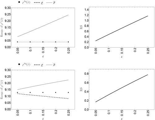
The following features can be obtained from a detailed examination of each plot in Figure 3 and are helpful for assessing the sensitivity of the feeling parameter, measured as its posterior mean: (1) taking a look at the maximum range of variation illustrates how the feeling parameter may respond to larger variations, and (2) analyzing the RS curve profile illustrates how the deviations have changed over $\epsilon ,$ providing an indicator of posterior sensitivity.

Figure 3 shows how the upper and lower bounds of both the models grow as $\epsilon$ increases. Moreover, the proposed rescaled shifted binomial-shifted beta model exhibits more robust behavior than the standard Poisson-gamma model. Its range of variation was smaller and its RS factor values were also significantly smaller. Similar results apply to the case of a small sample size ($n=10$), as shown in Figure 4.

Figure 4. Range of the posterior mean (left) and RS factor (right) for the Gstaad Hotel case, observed data $n=10$ and $x^{+}=82$. Poisson-gamma model (top panel) and rescaled shifted binomial-shifted beta model (bottom panel).

4.3.2. The Bellevire Gstaad hotel case

As shown in Table 3, the base priors to be contaminated are now a gamma distribution with parameters $\alpha =62.7$ and $\beta =7.84$ in the Poisson-gamma model, and a shifted beta distribution with parameters $\alpha =10$ and $\beta =3$ in the rescaled shifted binomial-shifted beta case, respectively. Similar to the Gstaad Hotel case, Figures 5 and 6 show the behavior of the upper and lower bounds and the RS factor under the very small sample size ($n=5$) and small sample size ($n=10)$ scenarios.

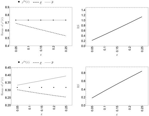
Figure 5. Range of the posterior mean (left) and RS factor (right) for the Bellevire Gstaad Hotel case, observed data $n=5$ and $x^{+}=46$. Poisson-gamma model (top panel) and rescaled shifted binomial-shifted beta model (bottom panel).

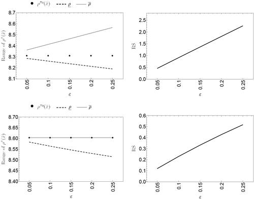
Figure 6. Range of the posterior mean (left) and RS factor (right) for the Bellevire Gstaad Hotel case, observed data $n=10$ and $x^{+}=82$. Poisson-gamma model (top panel) and rescaled shifted binomial-shifted beta model (bottom panel).

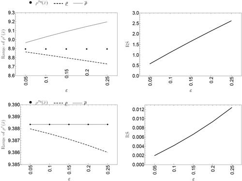
As in the previous case, the proposed model shows a more robust behavior than the Poisson case, presenting much lower RS-factor values. Note that the RS values for the Poisson model were almost four times higher than those obtained from the proposed model for large $\epsilon$ values.

When a small sample size is considered, the ranges in Figure 6 are notably reduced in our proposed model. Note that in this case, the RS values are well below the corresponding $\epsilon$ values, indicating the robustness of the proposed model. In this situation, the hospitality manager will have few doubts about the effects obtained from the ‘true’ benchmark prior.

5. Final comments

Bianchi and Heo (2021) have shown that Bayesian methods for hospitality research it is suitable for analyzing rating data when small sample sizes and expert judgements are present. A conjugated Poisson-gamma model was presented, and informally, they developed a sensitivity study of the posterior mean for prior information. However, in this study, we show that the Poisson-gamma model can be improved with the alternative rescaled shifted binomial-shifted beta model that appropriately captures the nature of the data, and, on the other hand, we introduce a robust Bayesian methodology (easily implementable from a computational point of view) that allows studying the sensitivity of the (posterior) average score value to the natural uncertainty that the hospitality manager may have in his expert judgement assignment.

Our interest is threefold: (i) we show that the proposed rescaled shifted binomial distribution is suitable for fitting rating data, (ii) we have shown how the practitioner can introduce his/her judgments about the feeling parameter $\mathrm{\theta }$ using an appropriate prior distribution. Intuitive concepts such as mode allow us to model the proper a priori distribution, but the expert cannot precisely express a single distribution that models his a priori judgments, and (iii) we also consider how our methodology allows us to manage this uncertainty in our model by using classes of prior distributions and how the measures of interest are transformed into intervals of interest that will enable the hospitality manager to make decisions.

Author contributions

Conceptualization, EGD and FJVP; methodology, EGD, MME, and FJVP; analysis and interpretation of the data, EGD, MME, and FJVP; drafting of the paper, EGD, and FJVP; writing, review, and editing, EGD, MME, and FJVP. All authors read and agreed to the final version of the manuscript.

Data and code availability

Data sets and codes are available from the online repository: https://github.com/fjvpolo/CBM.

Acknowledgements

The authors are grateful to two referees for a very careful reading of the manuscript and suggestions that improved the paper.

Disclosure statement

On behalf of all authors, the corresponding author states that there are no conflicts of interest.

Additional information

Funding

This work was partially supported by the Agencia Estatal de Investigación (Ministerio de Ciencia e Innovación, Spain) under Grant PID2021–127989OB-I00. Also, EGD was partially by grant TUR-RETOS2022-075 (Ministerio de Industria, Comercio y Turismo).

Notes on contributors

Emilio Gómez-Déniz

Emilio Gómez-Déniz PhD in Economics and Business Management, is a chair Professor in Mathematics at University of Las Palmas de Gran Canaria (Spain). Gómez-Déniz’s research focussed on Bayesian and Actuarial Statistics and in the areas of Tourism Management, Teaching Methodologies and Educational Innovation and Statistics Models in Sports. Gómez-Déniz is a member of the Institute of Tourism and Sustainable Economic Development (TiDES). He has widely published in top international journals on these topics, such as Insurance: Mathematics &amp; Economics, Tourism Economics, Current Issues in Tourism, among many others.

María Martel-Escobar

María Martel-Escobar is a full Professor in mathematics for economics and business at the Faculty of Economics, Business and Tourism, University of Las Palmas de Gran Canaria (ULPGC), Canary Islands, Spain. Prof. Martel–Escobar is a research member of the Tourism and Sustainable Economic Development (TIDES) Research Institute at the ULPGC. Martel–Escobar’s research focussed on applications of Bayesian methods to economics and business. Her recent publications appeared in leading applied statistics journals such as Journal of Applied Statistics, and Applied Stochastic Models in Business and Industry.

Francisco-José Vázquez-Polo

Francisco-José Vázquez-Polo is a Chair Professor of Bayesian Methods at ULPGC (Canary Islands, Spain) and research member of the TiDES Institute at the ULPGC. Prof. Vázquez–Polo is Head of the Department of Quantitative Methods at ULPGC. His research interests include Bayesian statistics as well as applications topics in economics, business and tourism. His work has been published in statistics and economic journals such as Statistical Methods in Medical Research, European Journal of Operational Research, Communications in Statistics: Theory and Methods, and Journal of Business and Economic Statistics, among others.

Notes

1 It is possible to alter the location and scale of the beta distribution of the first kind with pdf $f\left(x\right)=\frac{x^{\alpha -1}{\left(1-x\right)}^{\beta -1}}{B\left(\alpha ,\beta \right)}$ by introducing two further parameters representing the minimum, 1, and maximum m + 1, by a linear transformation substituting the non-dimensional variable $x$ in terms of the new variable $\theta$ with support in (1, m + 1).

Appendix

Technical details

Let the class of distributions be given by equation (11). It is clear that the posterior mean of $\theta$ is given by: $$\begin{array}{ccc}{\rho }^{\pi }\left(\tilde{x}\right)& =& \lambda \left(\tilde{x}\right){\rho }^{{\pi }_0}\left(\tilde{x}\right)+\left[1-\lambda \left(\tilde{x}\right)\right]{\rho }^q\left(\tilde{x}\right),\end{array}$$ where $\lambda \left(\tilde{x}\right)=\left(1-\epsilon \right)m\left(\tilde{x}|{\pi }_0\right)/m\left(\tilde{x}|q\right),$ being $m\left(\tilde{x}|{\pi }_0\right)=\Theta \left(\tilde{x}|\theta \right){\pi }_0\left(\theta \right)\hspace{0.17em}d\theta$ and $m\left(\tilde{x}|q\right)=\Theta \left(\tilde{x}|\theta \right)q\left(\theta \right)\hspace{0.17em}d\theta$.

Following the ideas provided in Sivaganesan (1991) and Gómez-Déniz et al. (2000), among others, it can be seen that the lower and upper bounds of the customers’ review can be obtained from, $$\begin{array}{c}\underset{\pi \hspace{0.17em}\in \hspace{0.17em}{\Gamma }_2}{\text{sup}}\left(\underset{\pi \hspace{0.17em}\in \hspace{0.17em}{\Gamma }_2}{\text{inf}}\right){\rho }^{\pi }\left(\tilde{x}\right)=\underset{z}{\text{sup}}\left(\underset{z}{\text{inf}}\right)\frac{a\left(\tilde{x}\right){\rho }^{{\pi }_0}\left(x\right)+r_2\left(z\right)}{a\left(\tilde{x}\right)+r_1\left(z\right)},\end{array}$$ where $$r_i\left(z\right)=\{\begin{array}{cc}\frac{1}{z}{{\displaystyle \int }}_{{\theta }_0}^{{\theta }_0+z}{b}_i\left(\theta \right),& z>0,\\ b_i\left({\theta }_0\right),& z=0,\end{array}$$ or $$r_i\left(z\right)=\{\begin{array}{cc}\frac{1}{z}{{\displaystyle \int }}_{{\theta }_0-z}^{{\theta }_0}{b}_i\left(\theta \right),& z>0,\\ b_i\left({\theta }_0\right),& z=0,\end{array}$$ depending on whether the bounds are reached when the contamination $q\left(\theta \right)$ is a uniform distribution $\left({\theta }_0,{\theta }_0+z\right)$ or $\left({\theta }_0-z,{\theta }_0\right)$, respectively, and (13) $$a\left(\tilde{x}\right)\hspace{0.17em}=\hspace{0.17em}\left(1-\epsilon \right)m\left(\tilde{x}{\pi }_0\right)/\epsilon ,$$(13) (14) $$b_i\left(\theta \right)\hspace{0.17em}=\hspace{0.17em}{\theta }^{i-1}f\left(\tilde{x}\theta \right),\hspace{0.17em}i=1,2.$$(14)

Rescaled shifted binomial-shifted beta model

$$\begin{array}{c}m\left(\tilde{x}{\pi }_0\right)=\frac{B\left(\alpha +x^{+}-n,\beta +\mathit{\text{nm}}-x^{+}+n\right)}{B\left(\alpha ,\beta \right)}{\displaystyle \prod }_{i=1}^n\left(\begin{array}{c}m\\ x_i-1\end{array}\right).\end{array}$$

Using the expressions given in (13(13) $$a\left(\tilde{x}\right)\hspace{0.17em}=\hspace{0.17em}\left(1-\epsilon \right)m\left(\tilde{x}{\pi }_0\right)/\epsilon ,$$(13) ) and (14$$\begin{array}{c}m\left(\tilde{x}{\pi }_0\right)=\frac{B\left(\alpha +x^{+}-n,\beta +\mathit{\text{nm}}-x^{+}+n\right)}{B\left(\alpha ,\beta \right)}{\displaystyle \prod }_{i=1}^n\left(\begin{array}{c}m\\ x_i-1\end{array}\right).\end{array}$$), we obtain $$\begin{array}{ccc}a\left(\tilde{x}\right)& =& \frac{1-\epsilon }{\epsilon }\frac{B\left(\alpha +x^{+}-n,\beta +\mathit{\text{nm}}-x^{+}+n\right)}{B\left(\alpha ,\beta \right)}{\displaystyle \prod }_{i=1}^n\left(\begin{array}{c}m\\ x_i-1\end{array}\right),\\ b_1\left(\theta \right)& =& \frac{1}{m^{\mathit{\text{nm}}}}{\left(\theta -1\right)}^{x^{+}-n}{\left(m+1-\theta \right)}^{\mathit{\text{nm}}-x^{+}+n}{\displaystyle \prod }_{i=1}^n\left(\begin{array}{c}m\\ x_i-1\end{array}\right),\\ b_2\left(\theta \right)& =& \frac{1}{m^{\mathit{\text{nm}}}}\theta {\left(\theta -1\right)}^{x^{+}-n}{\left(m+1-\theta \right)}^{\mathit{\text{nm}}-x^{+}+n}{\displaystyle \prod }_{i=1}^n\left(\begin{array}{c}m\\ x_i-1\end{array}\right).\end{array}$$

Poisson-Gamma model

Using the expressions given in (13(13) $$a\left(\tilde{x}\right)\hspace{0.17em}=\hspace{0.17em}\left(1-\epsilon \right)m\left(\tilde{x}{\pi }_0\right)/\epsilon ,$$(13) ) and (14$$\begin{array}{c}m\left(\tilde{x}{\pi }_0\right)=\frac{B\left(\alpha +x^{+}-n,\beta +\mathit{\text{nm}}-x^{+}+n\right)}{B\left(\alpha ,\beta \right)}{\displaystyle \prod }_{i=1}^n\left(\begin{array}{c}m\\ x_i-1\end{array}\right).\end{array}$$), we obtain $$\begin{array}{ccc}a\left(\tilde{x}\right)& =& \frac{1-\epsilon }{\epsilon }\frac{1}{{{\displaystyle \prod }}_{i=1}^n{x}_i!}\frac{{\beta }^{\alpha }\Gamma \left(\alpha +x^{+}\right)}{\Gamma \left(\alpha \right){\left(\beta +n\right)}^{\alpha +x^{+}}},\\ b_1\left(\theta \right)& =& \frac{1}{{{\displaystyle \prod }}_{i=1}^n{x}_i!}{\theta }^{x^{+}}\text{exp}\left(-n\theta \right),\\ b_2\left(\theta \right)& =& \frac{1}{{{\displaystyle \prod }}_{i=1}^n{x}_i!}{\theta }^{x^{+}+1}\text{exp}\left(-n\theta \right).\end{array}$$

References

- Assaf, A. (2009). Are U.S. airlines really in crisis? Tourism Management, 30(6), 916–921. https://doi.org/10.1016/j.tourman.2008.11.006
- Assaf, A. (2011). Accounting for technological differences in modelling the performance of airports: Bayesian approach. Applied Economics, 43(18), 2267–2275. https://doi.org/10.1016/j.tourman.2008.11.006
- Assaf, A. G. (2012). Benchmarking the Asia Pacific tourism industry: A Bayesian combination of DEA and stochastic frontier. Tourism Management, 33(5), 1122–1127. https://doi.org/10.1016/j.tourman.2011.11.021
- Assaf, A. G., & Tsionas, E. G. (2015). Incorporating destination quality into the measurement of tourism performance: A Bayesian approach. Tourism Management, 49, 58–71. https://doi.org/10.1016/j.tourman.2015.02.003
- Assaf, A. G., & Tsionas, M. (2018). Measuring hotel performance: Toward more rigorous evidence in both scope and methods. Tourism Management, 69, 69–87. https://doi.org/10.1016/j.tourman.2018.05.008
- Assaf, A. G., & Tsionas, M. G. (2019a). Quantitative research in tourism and hospitality: an agenda for best practice recommendations. International Journal of Contemporary Hospitality Management, 31(7), 2776–2787. https://doi.org/10.1108/IJCHM-02-2019-0148
- Assaf, A. G., & Tsionas, M. G. (2019b). Bayesian dynamic panel models for tourism research. Tourism Management, 75, 582–594. https://doi.org/10.1016/j.tourman.2019.06.012
- Assaf, A. G., & Tsionas, M. (2021). Bayesian hypothesis testing for hospitality and tourism research. Journal of Hospitality & Tourism Research, 45(6), 1114–1130. https://doi.org/10.1177/1096348020947327
- Assaf, A. G., Tsionas, M., & Oh, H. (2018). The time has come: Toward Bayesian SEM estimation in tourism research. Tourism Management, 64, 98–109. https://doi.org/10.1016/j.tourman.2017.07.018
- Berger, J. O. (1985). Statistical decision theory and bayesian analysis (2nd ed.). Springer.
- Bianchi, G., & Heo, C. Y. (2021). A Bayesian statistics approach to hospitality research. Current Issues in Tourism, 24(22), 3141–3150. https://doi.org/10.1080/13683500.2021.1896486
- Boto-García, D., Zapico, E., Escalonilla, M., & Baños Pino, J. F. (2021). Tourists’ preferences for hotel booking. International Journal of Hospitality Management, 92, 102726. https://doi.org/10.1016/j.ijhm.2020.102726
- Chang, V., Liu, L., Xu, Q., Li, T., & Hsu, C.-H. (2020). An improved model for sentiment analysis on luxury hotel review. Expert Systems, 40(2), e12580. https://doi.org/10.1111/exsy.12580
- Chen, K., Wang, P., & Zhang, H. (2021). A novel hotel recommendation method based on person- alized preferences and implicit relationships. International Journal of Hospitality Management, 92, 102710. https://doi.org/10.1016/j.ijhm.2020.102710
- Comerio, N., & Pacicco, F. (2021). Thank you for your staying! An analysis of the economic impact of tourism in Japanese prefectures. Current Issues in Tourism, 24(12), 1721–1734. https://doi.org/10.1080/13683500.2020.1801604
- Diaconis, P., & Ylvisaker, D. (1979). Conjugate priors for exponential families. The Annals of Statistics, 7(2), 269–281. https://doi.org/10.1214/aos/1176344611
- D’Elia, A., & Piccolo, D. (2005). A mixture model for preferences data analysis. Computational Statistics & Data Analysis, 49(3), 917–934. https://doi.org/10.1016/j.csda.2004.06.012
- Ericson, W. (1969). A note on the posterior mean of a population mean. Journal of the Royal Statistical Society Series B: Statistical Methodology, 31(2), 332–334. https://doi.org/10.1111/j.2517-6161.1969.tb00794.x
- Fang, B., Ye, Q., Kucukusta, D., & Law, R. (2016). Analysis of the perceived value of online tourism reviews: Influence of readability and reviewer characteristics. Tourism Management, 52, 498–506. https://doi.org/10.1016/j.tourman.2015.07.018
- Fong, L. H. N., Lam, L. W., & Law, R. (2017). How locus of control shapes intention to reuse mobile apps for making hotel reservations: Evidence from Chinese consumers. Tourism Management, 61, 331–342. https://doi.org/10.1016/j.tourman.2017.03.002
- Gómez-Déniz, E., Hernández-Bastida, A., & Vázquez-Polo, F. J. (2000). Robust Bayesian premium principles in actuarial science. Journal of the Royal Statistical Society (the Statistician, Series D), 49(2), 241–252.
- Hoffart, J. C., Olschewski, S., & Rieskamp, J. (2019). Reaching for the star ratings: A Bayesian inspired account of how people use consumer ratings. Journal of Economic Psychology, 72, 99–116. https://doi.org/10.1016/j.joep.2019.02.008
- Lee, P. M. (1997). Bayesian statistics. An introduction (2nd ed.). Arnold.
- Lei, S. S. I., Nicolau, J. L., & Wang, D. (2019). The impact of distribution channels on budget hotel performance. International Journal of Hospitality Management, 81, 141–149. https://doi.org/10.1016/j.ijhm.2019.03.005
- Li, S., & Chen, J. (2023). Mixture of shifted binomial distributions for rating data. Annals of the Institute of Statistical Mathematics, 75(5), 833–853. https://doi.org/10.1007/s10463-023-00865-7
- Martel-Escobar, M., González-Martel, C., & Vázquez-Polo, F. J. (2023). Managing score heterogene- ity between online consumer review websites. Cogent Social Sciences, 9(2), 2267261. https://doi.org/10.1080/23311886.2023.2267261
- Mellinas, J. P., María-Dolores, S.-M. M., & Bernal García, J. J. (2015). Booking.com: The unex- pected scoring system. Tourism Management, 49, 72–74. https://doi.org/10.1016/j.tourman.2014.08.019
- Mellinas, J. P., María-Dolores, S.-M. M., & Bernal García, J. J. (2016). Effects of the Booking.com scoring system. Tourism Management, 57, 80–83. https://doi.org/10.1016/j.tourman.2016.05.015
- Mellinas, J. P., & Martin-Fuentes, E. (2021). Effects of Booking.com’s new scoring system. Tourism Management, 85, 104280. https://doi.org/10.1016/j.tourman.2020.104280
- Nilashi, M., Ahani, A., Esfahani, M. D., Yadegaridehkordi, E., Samad, S., Ibrahim, O., Sharef, N. M., & Akbari, E. (2019). Preference learning for eco-friendly hotels recommendation: A multi- criteria collaborative filtering approach. Journal of Cleaner Production, 215, 767–783. https://doi.org/10.1016/j.jclepro.2019.01.012
- O’Hagan, A., Buck, C. E., Daneshkhah, A., Eiser, J. :R., Garthwaite, P. H., Jenkinson, D. J., Oakley, J. E., & Rakow, T. (2006). Uncertain judgements: Eliciting experts’ probabilities. Wiley.
- Peng, H.-G., Zhang, H.-Y., & Wang, J.-Q. (2018). Cloud decision support model for selecting hotels on TripAdvisor.com with probabilistic linguistic information. International Journal of Hospi- Tality Management, 68, 124–138.
- Pérez, C. J., Martín, J., & Rufo, M. J. (2006). Sensitivity estimations for Bayesian inference models solved by MCMC methods. Reliability Engineering & System Safety, 91(10-11), 1310–1314. https://doi.org/10.1016/j.ress.2005.11.029
- Ríos, D., & Ruggeri, F. (2000). Robust bayesian analysis (Lecture Notes in Statistics). Springer- Verlag.
- Simone, R. (2021). An accelerated EM algorithm for mixture models with uncertainty for rating data. Computational Statistics, 36(1), 691–714. https://doi.org/10.1007/s00180-020-01004-z
- Sivaganesan, S. (1991). Sensitivity of some posterior summaries when the prior is unimodal with specified quantiles. Canadian Journal of Statististics, 19, 57–65.
- Stefan, A. M., Katsimpokis, D., Gronau, Q. F., & Wagenmakers, E. J. (2022). Expert agreement in prior elicitation and its effects on Bayesian inference. Psychonomic Bulletin & Review, 29(5), 1776–1794. https://doi.org/10.3758/s13423-022-02074-4
- Vázquez, F. J., Moreno, E., Negrín, M. A., & Martel, M. (2016). Bayesian robustness in meta-analysis for studies with zero responses. Pharmaceutical Statistics, 15(3), 230–237. https://doi.org/10.1002/pst.1741
- Watson, J. M., & Moritz, J. B. (2000). The longitudinal development of understanding of average. Mathematical Thinking and Learning, 2(1-2), 11–50. https://doi.org/10.1207/S15327833MTL0202_2
- Winkler, R. L. (1968). The assessment of prior distributions in Bayesian analysis. Journal of the American Statistical Association, 62(319), 776–800. https://doi.org/10.2307/2283671
- Xiang, Z., Du, Q., Ma, Y., & Fan, W. (2017). A comparative analysis of major online review plat- forms: Implications for social media analytics in hospitality and tourism. Tourism Management, 58, 51–65. https://doi.org/10.1016/j.tourman.2016.10.001
- Zellner, A., & Siow, A. (1980). Posterior odds ratios for selected regression hypotheses. TEST, 31, 585–603.
- Zhao, Y., Xu, X., & Wang, M. (2019). Predicting overall customer satisfaction: Big data evidence from hotel online textual reviews. International Journal of Hospitality Management, 76, 111–121. https://doi.org/10.1016/j.ijhm.2018.03.017