Prioritization of CIFs taking into account multiple criteria for the construction of efficient portfolios

Abstract

This study presents a methodology for making decisions on the number of Collective Investments Funds (CIF) for portfolio construction using Multi-Criteria Decision Analysis (MCDA) techniques, particularly a combination called PrAToVi. The proposed methodology includes the integration of economic and financial theories of investment in equity portfolios with the multi-criteria techniques described in PrAToVi, which allows a finite number of alternatives to be evaluated hierarchically under qualitative and quantitative criteria. This methodology was evaluated with funds managed by fiduciaries and with information from the end of 2021, which is contained in the technical sheets of each fund, and, the compares with information about 2022 and 2023. The computational results show the importance and efficiency of successfully integrating traditional investment criteria in stock portfolios and multi-criteria methodologies to generate a ranking of those CIFs with which portfolios can be created and an adequate balance between multiple criteria, including profitability and risk, can be found. This approach also considers the investment decision-making process regarding assets managed by Colombian SFs. The proposed methodology can be applied to other emerging markets such as Colombia and can manage this alternative type of investment.

Keywords:

• Prioritization
• collective investments funds
• alternatives investments
• portfolio construction
• MCDA

Reviewing Editor:

• David McMillan, University of Stirling, United Kingdom of Great Britain and Northern Ireland

Subjects:

• quantitative finance
• decision analysis
• financial management

1. Introduction

There are many mechanisms through which to invest money; most investors commonly look for a portfolio composed of stocks that have high-level returns and low-level volatility. In recent decades, the increasing degree of competition among companies, financial institutions, and organizations, globalization of financial markets, rapid economic and social evolution, and technological changes have led to an increase in uncertainty and instability in finance and business environments. According to Doumpos (2018), the main areas of interest in the literature are corporate finance, financial economics, behavioral finance, valuation, risk management, and financial engineering.

In this new context, the importance of making efficient financial decisions and the complexity of the financial decision-making process have increased (Constantin Zopounidis & Doumpos, 2002). This complexity is evident in the existing variety and volume of new financial resources, products and services.

Financial professionals and researchers in these fields recognize the need to address financial decision-making problems through integrated and realistic approaches based on sophisticated quantitative analysis techniques. Therefore, the connection between financial theory and mathematical modelling has become evident, which has led to financial decision-making becoming analytical with a high level of modelling and methodological sophistication (Doumpos, 2018).

In parallel, investments in non-traditional assets have been gaining importance worldwide in recent decades because this type of investment can offer interesting returns and opportunities for portfolio diversification, thus contributing to a reduction in the degree of inherent risk of the activity. According to Lopez and Hurtado (2008), this type of investment has emerged as a response to the lack of profitability of traditional investments, such as a fall in the yield of government bonds. As a result, investors have progressively built an important part of institutional investment portfolios—mutual and pension funds.

Because sophisticated investors witnessed the poor performance of traditional investments, many turned to alternative investments to meet their return objectives and a means of controlling risk. For example, as noted by Baker and Filbeck (2013), alternative investments provide the opportunity to obtain a reasonable return with a manageable level of risk. Some alternative investments offer opportunities to participate in different markets and apply investment strategies that are not available to the general investing public. According to some researchers (P. Chen et al., 2011), (Amin & Kat, 2003), (H. C. Chen et al., 2005) and (Anson, 2002), these types of investments achieve superior performance in terms of the inclusion of alternative investments independently or as part of a portfolio composed of traditional assets.

The remainder of this paper is structured as follows: Section 2 presents the literature review. Section 3 explains the study’s research methodology, a section will consist of the results and discussion. Finally, Section 5 concludes the study.

2. Literature review

2.1. Optimal portfolio theory

The use of theory for the optimal selection of efficient portfolios originated from (Markowitz, 1959) and has been enriched with essential contributions, such as those of Sharpe (1964) and (Stephen, 1976), among other authors who have made significant progress in terms of the problems that stand out in portfolio selection decisions, especially concerning the choice of indices or criteria to be considered.

As described by Loraschi and Tettamanzi (2002), the central problem of portfolio theory concerns the selection of asset weights in a portfolio that minimize a certain measure of risk for any given level of expected return. To construct an optimal portfolio, (Markowitz, 1959) suggested minimizing the risk of the portfolio at a certain level of its expected return. This model is called the variance-mean model and is widely used because of its ease of use and simplicity. In (Loraschi & Tettamanzi, 2002)) the autors explained that Markowitz proposed the use of “seivmariance”, defined as the weighted average of the squared distances of the returns below the mean of the distribution, as an index of risk, due realizing that the investor perceives risk only on the downside part of the return distribution.

Likewise, as described in Prigent (2007), since Markowitz introduced a seminal analysis of mean-variance in 1959, portfolio management theory has been expanded to consider different characteristics:

Dynamic optimization of the portfolio according to Merton

• Choice of new decision criteria based on risk aversion (utility functions) or risk measures (value at risk (VaR), conditional VaR (CvaR), etc.).

• Market imperfections, such as transaction costs and

• Specific portfolio strategies, such as portfolio insurance or alternative methods (hedge funds).

However, as mentioned in Kim et al. (2014), the model is highly sensitive to its inputs due to the random nature of asset returns. According to Black and Litterman (1992), assets often have unintuitive or extreme weights, such as investment positions with large negative weights, which cannot be considered in active trading. Other approaches have been reported in the literature, such as the mean absolute deviation (MAD) found by Konno and Yamazaki (1991) and the CVaR approach reviewed by Rockafellar and Uryasev (2000). In the above three studies, the measure for returns (yields) is the average and what varies is the measure for risk (variance, MAD, and CVaR). Another approach explained by Doumpos and Grigoroudis (2013) is the upside deviation-downside deviation (UD-DD) approach, which uses terms used by financial investors known as “good volatility” and “bad volatility.” As a novelty, in order to select the optimal portfolio, in García et al. (2020) the authors extends the stochastic mean-semivariance model to a fuzzy multiobjective model, Particularly, it optimizes the expected return, the semivariance and the cardinality constraint and upper and lower bound constraints; defining the credibilistic Sortino ratio as the ratio between the credibilistic risk premium and the credibilistic semivariance. The constrained portfolio optimization problem resulting is solved using the algorithm NSGA-II. In (Brandtner et al., 2020) they incorporate the concept of convex shortfall risk measures in portfolio optimisation. Additionally, in García et al. (2022) they construct pareto efficient portfolios using a fuzzy multicriteria portfolio selection model with real-world constraints. Recently, in Huang and Ma (2023) using uncertainty theory, the authors discusses a portfolio selection problem considering inflation, a most popular multiplicative background risk, in such situations, and analyses the effect of uncertain inflation on investment in risky and risk-free assets.

2.2. MCDA and portfolio selection

Considering the wide variety of objectives that are part of the optimization process that the investor must conduct, the use of multi-criteria decision analysis (MCDA) is both relevant and versatile. For example, in search of delimiting the problem and some methods used in the present study (Bahmani et al., 1987) applied the analytic hierarchy process (AHP) to the asset selection process for a given investment. Zopounidis in C. Zopounidis (1999), the contribution of MCDA to the resolution of financial decision problems.

According to Xidonas et al. (2009), who focused on the selection of assets through a specific method, the relevance of the use of MCDM is reinforced. This study argues that the MCDM paradigm provides a broad methodological approach for effectively addressing portfolio selection problems.

Some of the first papers published on the selection of equity portfolios and using multi-criteria methods were those of Hababou and Martel (1998), (Costa et al., 2004) and (Bouri et al., 2002).

In (Hababou & Martel, 1998), a methodology comprising the following four stages: (1) defining a list of potential solutions to the problem considered, (2) defining a list of critical criteria, (3) evaluating the performance of each solution according to each criterion, and (4) aggregating these returns using the PROMETHEE II multi-criteria method.

(Costa et al., 2004) presented a model for selecting a portfolio based on the results of fund managers’ fieldwork and using direct scoring, optimization, and MACBETH techniques.

In (Bouri et al., 2002), the authors included the investor’s attitude toward solvency and liquidity, solving a portfolio problem with a multi-criteria issue, which must be addressed using appropriate techniques.

In (Vásquez et al., 2021), a hybrid method between two multi-criteria techniques applied directly to the optimal selection of financial portfolios in search of a more robust and complete optimization process was proposed. This process is one of the most decisive criteria or objectives for investors.

2.3. Alternative investments

Alternative investments are vital in large investment portfolios worldwide, especially in emerging countries. Likewise, owing to the lack of structured information on this type of investment, the large portfolios of institutional entities, such as pension funds and trust funds, have adopted the position of investors with ends and not means. That is, large portfolios do not guarantee profitability, but depend on the performance of the investments within.

According to P. Chen et al. (2011), this type of investment seeks greater profitability by including alternative investments in isolation or as part of a portfolio comprising traditional assets. In (Baker & Filbeck, 2013), these types of investment into two large groups:

• Traditional alternative investments: This group includes real estate, private capital, raw materials and

• Modern alternative investments: This group includes managed futures, hedge funds, and distressed securities of companies or government entities that are already in default, under bankruptcy protection, in danger, or heading toward such a condition. The most common types of distressed securities are bonds and bank debts.

In addition, emerging alternative investments present highly important research topics related to information asymmetry and agency costs, governance and monitoring, and legal and economic conditions (Cumming & Zhang, 2016). According to Begué Hoyos (2012), to define alternative investments, traditional ones must first be delimited. When discussing these investments, reference is made to stocks (variable income), bonds, treasury bonds (TESs), or certificates of deposit (CDs), as they are considered traditional because they are the most common options people use to invest their money. As alternative types of investment, reference mades to private equity funds (FCPs), real estate funds (real estate investment trusts (REITs)), commodities, and hedge funds) and a special type of “speculative” collective portfolio called a collective investment fund (CIF).

2.4. CIF’s in Colombia

According to (Decreto 2555, 2555, 2010), “collective speculation portfolios are understood to be those whose primary objective is to carry out operations of a speculative nature, including the possibility of carrying out operations for amounts greater than those contributed by investors (leverage)”. Later, in Decreto 1242, 1242 (2013) defined CIFs as “any mechanism or vehicle for the collection or administration of sums of money or other assets.” CIFs defined as the mechanisms or vehicles through which to capture or manage sums of money or other assets with the contributions of many people, which can be determined once the fund is operational. In addition, CIFs collectively manage resources to obtain collective economic results (Asociación de Fiduciarias de Colombia, 2013).

In Colombia, financing assets in a capital market can be segmented as a) individual administration, headed by the client, and b) delegated administration, which can occur through individual or collective investment vehicles. According to Maiguashca (2016), in the first case, investors act on their own and can count on an intermediary to carry out market transactions on their behalf and on some type of agent to act as a depositary for their investments. However, investment and ownership decisions are concentrated on investors themselves. In the second case, a professional manager makes investment decisions within a general mandate defined by the client who acts as the principal. This mandate can be from a client, in which case, it is considered an individual delegated administration. The individual management actors offered by the Colombian market are fundamentally third-party portfolio managers of stock brokerage companies (SBCs) and individual investment trusts of trust companies (SFs).

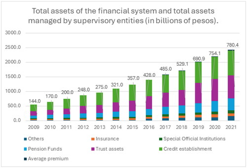
According to Asofiduciarias (2021), at the end of 2019, managed assets were distributed to more than 24,900 businesses, a figure that increased by 1% compared to that at the end of the previous year. The trust sector manages approximately 690 billion pesos in assets, with an annual growth of 19%. The income from the administration of these businesses amounted to $ 1.88 billion, representing an increase of 12%. Conversely, the profits of the trust sector grew by 33%, exceeding 710,000 million pesos. IIn 2021, the fiduciary sector took advantage of economic recovery to continue articulating businesses in the different sectors of the economy. As a result, the assets managed by the sector exceeded $700 billion through 25,257 businesses, with the last figure being registered as a historical record in terms of the number of businesses managed by fiduciaries.

Figure 1 shows the evolution of the assets managed by SFs, which show constant growth.

Figure 1. Total assets of the financial system and total assets managed by supervisory entities (in billions of pesos).

Source: Own elaboration from the annual information of Asofiduciarias.

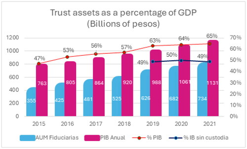
As of December 2021, assets under management represent 65% of gross domestic product (GDP), as shown in Figure 2.

Figure 2. Trust assets as a percentage of GDP.

Source: Annual report of Asofiduciarias (2021).

Within the obligations of CIF management companies, they keep investors informed, at least through the following mechanisms.

• Regulation

• Prospectus

• Technical data

• Investor account statement

• Accountability report

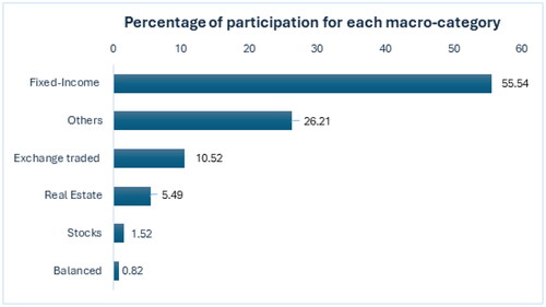
The System of Categorization of CIFs (SICIF) consists of establishing homologous groups of CIFs so that they are objectively comparable and allow the investor to know, evaluate, and make decisions about which funds best suit the needs of the investor (Asofiduciarias et al., 2021). The CIF, for improved administration and monitoring, can be categorized into six macro categories. Figure 3 shows the percentage share of each macro category in the total assets under management at the end of January 2022.

Figure 3. Total assets managed by CIFs.

Source: Quarterly report of CIFs (Asofiduciarias et al., 2021).

Considering the above factors, the objective of this research was to generate a ranking that would allow the prioritization of these funds based on the technical information available for each CIF and through a combination of methodologies for multi-criteria decision-making (MCDM) and help in the construction of optimal portfolios for this type of investment in Colombia.

3. Methodology

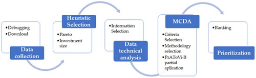
The proposed methodology for the development of this study is divided into five stages, which are summarized in Figure 4.

Figure 4. Proposed methodology.

Source: Own elaboration.

3.1. Stage 1: Data collection

3.1.1. Download

Information on CIFs was collected from the Asofiduciarias website, which groups together the SFs who have been authorized to manage this type of investment in Colombia and have reported information since 2017. Information was downloaded individually for each entity.

3.1.2. Debugging

For data purification, the “extract, transform, load” (ETL) data-processing methodology was used. According to Duque Méndez et al. (2016), the activities of this methodology are framed as key activities in the context of databases because, through their combination, they allow for the transfer of data from one source to another.

3.2. Stage 2: Heuristic selection

At the time of this research, approximately 400 funds had been managed by 18 trust companies. Each trust company can manage any number of funds, as long as they are categorized in one of the 6 currently established macro-categories. For the heuristic selection, funds were selected from each trust company that accounted for at least 80% of the total funds under management, regardless of the number of assets under management. In the end, 72 funds were selected from the 18 trust companies.

3.3. Stage 3: Analysis of technical data

In (Decreto 2555, 2555, 2010) established the technical file as one of the mechanisms through which management companies can keep investors informed about all aspects inherent to CIFs. Likewise, the Ministerio de Hacienda Pública defines a technical file as a standardized information document for CIFs that contains the basic information of each fund that must be updated and published monthly within five (5) business days following the last calendar day of the month. The information cut-off date was the last calendar day of the month being reported. Similarly, SICIF determined the categorization summarized in Table 1.

Table 1. Categories and subcategories of CIFs in Colombia.

MACRO CAT	CAT	MACRO CAT	CAT
Fixed-Income Funds	High-Performance Weights	1	1
	Fixed-Income Pesos Liquidity	1	2
	National Fixed-Income Public Entities	1	3
	Short-Term Fixed Income Pesos	1	4
	Medium-Term Fixed-Income Pesos	1	5
	Long-Term Fixed-Income Pesos	1	6
	International Fixed-Income Funds	1	7
Stock Funds	National Stock Funds	2	1
	International Stock Funds	2	2
Balanced Funds	Balanced Funds with Lower Risk	3	1
	Moderately Balanced Funds	3	2
	Balanced Funds with Higher Risk	3	3
Exchange traded funds	Beta Stock Exchange Funds	4	1
	Smart Beta Stock Exchange Funds	4	2
Real Estate Funds	National Development Real Estate Funds	5	1
	National Income Real Estate Funds	5	2
Other Funds	Credit Asset Funds	6	1
	Other Equity Funds	6	2
	Other Funds	6	3

Source: Own elaboration.

In total, 6 macro categories and 19 micro categories were established.

3.4. Stage 4: Multi-criteria analysis

The purpose of this stage is to form the initial matrix, which identifies and summarizes the essential elements for the application of multi-criteria methodologies.

3.5. Initial matrix formation

3.5.1. Selection of criteria

In this study, the selected criteria have been validated and are available in the quarterly reports of all funds under evaluation. Accordingly, three dimensions have been established to categorize the criteria:

• Financial dimension: This encompasses three criteria: Profitability (C1), Risk (C2), and Fund Value (C3), which specifically evaluate financial performance and the size of the fund.

• Operational dimension: This includes two criteria that assess the fund’s operations, namely the number of investors (C4) and the average investment duration (C5).

• Administrative dimension: This consists of two criteria that appraise the credit rating (C6) and the manager’s experience (C7).

3.5.2. Selection of alternatives

Alternatives are the units or objects that serve as options to achieve the objective or solve the problem. In our research, these alternatives will be represented by the various funds.

3.5.3. Determination of performance indicators

The evaluation for each alternative must consider all attributes connected from the point of view considered pertinent. Considering what is described in Manyoma-Velásquez (2022), to make this comparison, it was essential to measure the performance of each action based on these criteria. Performance can be measured in diverse ways, through grades and scores, characterized by a number, or by being a verbal statement, among others.

3.6. Selection of the methodology

The most traditional approach in the multi-criteria world is to use a method to obtain an order or hierarchy of the alternatives analyzed, to make decisions in accordance with the possibilities of the decision-making center. The decision process includes evaluating the possible alternatives and choosing the best one.

But from this traditional application, some questions arise that haunt decision-makers after performing these procedures: is there a method that makes more sense than another method for a particular problem, and therefore leads to a better solution than another method? According to Romero (2000) the answer is far from easy, as the decision-making construction of each of them is different and this can lead to problems of comparison.

In (Manyoma-Velásquez, 2022), a methodology was suggested that allowed for adding the rankings generated by four (4) very common methods in the current literature: PROMETHEE II, Analytic Hierarchy Process (AHP), Technique for Order of Preference by Similarity to Ideal Solution (TOPSIS) and VIekriterijumsko KOmpromisno Rangiranje (VIKOR). This new method of adding results allows for a single hierarchy to be defined through another method, the Borda count.

3.7. Relative PrAToVi-B application

The method proposes the use of four multi-criteria decision analysis methods, which generate their own rankings and will be collected in a Borda count to obtain a unique ranking. As a first step, equal weights were determined for each of the seven criteria for the starting matrices of each methodology. Later, it was determined that the PrAToVi methodology could be applied using PROMETHEE II, TOPSIS, and VIKOR.

According to Manyoma-Velásquez (2022), the steps of each methodology are described below.

3.7.1. PROMETHEE II (7 steps)

PROMETHEE II (full classification) was developed by Jean-Pierre Brans and was first presented in 1982 at a conference organized by the Université Laval, Québec, Canada (Brans & De Smet, 2016). The basic structure is as follows.

• Step 1. In the initial decision matrix, the weights (importance) and the sense of the criterion (minimization or maximization) are located.

• Step 2. Normalize the matrix. Here, the method proposes linear normalization by interval, as shown in the following equations: (1) $$n_{\text{ij}}=\frac{\left[X_{\text{ij}}-\mathit{\text{min}}\left(X_{\text{ij}}\right)\right]}{\left[\mathit{\text{max}}\left(X_{\text{ij}}\right)-\mathit{\text{min}}\hspace{0.17em}\left(X_{\text{ij}}\right)\right]};\mathit{\text{maximization}}{n}_{\text{ij}}=\frac{\left[\mathit{\text{max}}\left(X_{\text{ij}}\right)-X_{\text{ij}}\right]}{\left[\mathit{\text{max}}\left(X_{\text{ij}}\right)-\mathit{\text{min}}\hspace{0.17em}\left(X_{\text{ij}}\right)\right]};\mathit{\text{minimization}}$$(1)

where $n_{\mathit{\text{ij}}}$ represents the normalized alternative and Xij is the value of the comparison previously obtained in the original matrix.

• Step 3. Calculate the differences (d). The differences between all alternatives must be established based on each criterion through pairwise comparisons. (2) $$\hspace{0.17em}d\left(a,b\right)\hspace{0.17em}=\hspace{0.17em}{C}_j\left(a\right)\hspace{0.17em}-C_j\left(b\right);$$(2)

• Step 4. Preference function (P) was calculated. The value of the preference function P is always between 0 and 1 and is calculated for each criterion. (3) $$P_j\left(a,b\right)=0\text{\hspace{0.17em}\hspace{0.17em}if\hspace{0.17em}\hspace{0.17em}d}\left(a,b\right)\hspace{0.17em}\le \hspace{0.17em}0;\text{\hspace{0.17em}\hspace{0.17em}and\hspace{0.17em}\hspace{0.17em}}{P}_j\left(a,b\right)=C_j\left(a\right)-C_j\left(b\right)\text{\hspace{0.17em}\hspace{0.17em}if\hspace{0.17em}\hspace{0.17em}d\hspace{0.17em}}\left(a,b\right)>0\hspace{0.17em}$$(3)

• Step 5. Calculate the aggregate preference, which shows how much alternative a is preferred over b, taking into account all criteria. This value ranges between 0 and 1, where W represents the importance given to each criterion. In this case, it was started with equal weights, and other assignments were evaluated through scenarios. (4) $$\pi (a,b)=\sum _{j=1}^n{,}_j{P}_j(\mathrm{a},\mathrm{b})$$(4)

• Step 6. Calculate the positive and negative upper flows, which are also called upper inflows and outflows, respectively. (5) $$\hspace{0.17em}{\phi }^{+}=\frac{1}{m-1\hspace{0.17em}}{\displaystyle \sum }_{b=1}^m\pi \left(a,b\right)\left(a\ne b\right);y{\phi }^{-}\frac{1}{m-1\hspace{0.17em}}\hspace{0.17em}{\displaystyle \sum }_{b=1}^m\pi \left(a,b\right)\left(a\ne b\right);m\mathit{\text{is}}\mathit{\text{the}}\mathit{\text{size}}\mathit{\text{of}}\mathit{\text{the}}\mathit{\text{matrix}}$$(5)

• Step 7. Calculate the net flow of the classification. The order of each alternative is based on the difference between (positive and negative). A higher value indicated a better alternative. (6) $$\phi \left(a\right)={\phi }^{+}\left(a\right)-\hspace{0.17em}{\phi }^{-}\left(a\right)$$(6)

3.7.2. TOPSIS (6 steps)

This method was first presented in 1981 by Hwang and Yoon (1981), who defined the following steps.

• Step 1. In the initial decision matrix, the weights (importance) and the sense of the criterion (minimization or maximization) are located.

• Step 2. Normalize the matrix. In this case, the method proposes the normalization of vectors, which is carried out using the following equation, where $n_{\mathit{\text{ij}}}$ represents the normalized alternative and xij is the value of the comparison previously obtained in the original matrix. (7) $${\overline{n}}_{\mathit{\text{ij}}}=\frac{x_{\mathit{\text{ij}}}}{\sqrt{\sum _{j=1}^m{\left(x_{\mathit{\text{ij}}}\right)}^2}},j=1,\dots n;i=1,\dots ,m$$(7)

• Step 3: Construct the weighted normalized decision matrix, where $w_j$ represents the importance assigned to each criterion, which in this case is based on Shannon entropy. (8) $${\overline{v}}_{\mathit{\text{ij}}}=w_j*{\overline{n}}_{\mathit{\text{ij}}},j=1,\dots ,n;i=1,\dots ,m$$(8)

• Step 4: Determine the ideal and negative solutions, which are the positive and negative ideal sets of values, ­respectively, represented as follows, where J is associated with the maximization criteria and J’ is associated with the minimization criteria: (9) $${\overline{A}}^{+}=\left\{{\overline{v}}_1^{+},\dots {\overline{v}}_n^{+}\right\}=\left\{\frac{({\text{max}}_i{\overline{v}}_{\mathit{\text{ij}}},j\in J)}{({\text{min}}_i{\overline{v}}_{\mathit{\text{ij}}},j\in J\prime )}\right\};y{\overline{A}}^{-}=\left\{{\overline{v}}_1^{-},\dots {\overline{v}}_n^{-}\right\}=\left\{\frac{({\text{min}}_i{\overline{v}}_{\mathit{\text{ij}}},j\in J)}{({\text{max}}_i{\overline{v}}_{\mathit{\text{ij}}},j\in J\prime )}\right\}$$(9)

• Step 5: Calculate the distance measurements. How far is each alternative from the “best” option and the “worst” option identified through Euclidean distances? (10) $${\overline{d}\mathrm{ }}_i^{+}+{\left\{\sum _{j=1}^n{\left({\overline{v}}_{\mathit{\text{ij}}}-{\overline{v}}_i^{+}\right)}^2\right\}}^{\frac{1}{2}};\text{y}{\overline{d}}_i^{-}+{\left\{\sum _{j=1}^n{\left({\overline{v}}_{\mathit{\text{ij}}}-{\overline{v}}_j^{-}\right)}^2\right\}}^{\frac{1}{2}}$$(10)

• Step 6: Calculate the relative proximity to the ideal solution and order preferences. Relative proximity R_i to the ideal solution is calculated as follows: (11) $${\overline{R}}_i=\frac{\overline{d}{\hspace{0.17em}}_i^{-}}{\overline{d}{\hspace{0.17em}}_i^{+}+{\overline{d}}_i^{-}},i=1,\dots .m;\mathit{\text{Si}}\overline{R}{\hspace{0.17em}}_i=1\to \mathit{\text{Ai}}={\overline{A}}^{+}\hspace{0.17em}\mathit{\text{Si}}\hspace{0.17em}\overline{\overline{R}}\hspace{0.17em}i=0\to \mathit{\text{Ai}}=\overline{A}-\hspace{0.17em}$$(11)

For the ordering of preferences, the closer to 1 the value of R_i is, the higher the priority of the corresponding ith alternative.

3.7.3. VIKOR (6 steps)

At the end of the 1980s, Serafim Opricovic established this method and defined the following steps (Opricovic & Tzeng, 2004):

• Step 1. In the initial decision matrix, the weights (importance) and the sense of the criterion (minimization or maximization) are located.

• Step 2. Determine the best and worst values for each criterion, depending on whether maximization or minimization is used. (12) $$\mathit{\text{Para Max}}:f_i^{+}=\mathit{\text{ma}}{x}_j{f}_{\mathit{\text{ij}}};f_i^{-}=\mathit{\text{mi}}{n}_j{f}_{\mathit{\text{ij}}};\mathit{\text{Para Min}}:f_i^{+}=\mathit{\text{mi}}{n}_j{f}_{\mathit{\text{ij}}};f_i^{-}=\mathit{\text{ma}}{x}_j{f}_{\mathit{\text{ij}}};$$(12)

• Step 3. Calculate the values of S_i and R_i, where the former represents the maximum group utility (“majority” rule) and the latter represents a minimum level of individual regret from the “opponent”. Here, w_j represents the importance given to each criterion, which, in this case, is through Shannon entropy. (13) $$S_i={\displaystyle \sum }_{i=1}^n{w}_j\frac{\left(f_i^{+}-f_{\mathit{\text{ij}}}\right)}{\left(f_i^{+}-f_j^{-}\right)};R_i=\mathit{\text{ma}}{x}_j\left[w_j\frac{\left(f_i^{+}-f_{\mathit{\text{ij}}}\right)}{\left(f_i^{+}-f_j^{-}\right)}\right]$$(13)

• Step 4. Calculate, which represents the ratio of the maximum utility of the group to the individual’s opposition to the compromised solution. v denotes a group’s maximum utility weight and (1-$v$) is the weight of the individual opposition. Parameter v takes values between zero and one. A value of $v$ = 0.5 implies a consensus strategy between the two positions. If $v$ <0.5, then the minority decides; that is, the individual position is of greater importance. If $v$ > 0.5, the majority decide. (14) $$Q_i=v\hspace{0.17em}\frac{\left(S_i-S^{+}\right)}{\left(S^{-}-S^{+}\right)}+\left(1-v\right)\left(\frac{R_i-R^{+}}{R^{-}-R^{+}}\right);\text{\hspace{0.17em}donde\hspace{0.17em}}{S}^{+}=\mathit{\text{min}}\hspace{0.17em}{S}_i,S^{-}=\mathit{\text{max}}{S}_i,R^{+}=\mathit{\text{min}}\hspace{0.17em}{R}_i,R^{-}=\mathit{\text{max}}{R}_i\hspace{0.17em}$$(14)

• Step 5. The alternatives are ordered in descending order according to ${ S}_i$, ${ R}_i$, and ${ Q}_i$. This ranking index is an aggregation of all criteria, the relative importance of the criteria, and the balance between the total and individual satisfaction. The minimum $Q_i$ represents the best alternative.

• Step 6. Propose a compromised solution. The best-ranked alternatives (minimum Q) are proposed if the following two conditions are satisfied: Condition 1: Acceptable advantage, where m represents the total number of alternatives. The difference between Alternatives 2 and 1 must be greater than the value obtained (fixed) by dividing the unit by the number of alternatives. Condition 2: Acceptable stability in decision-making. Alternative A1 must also be the best-ranked alternative, classified as S or R. If one of the two conditions is not met, then a set of compromised solutions is proposed that consists of the following: a) if Condition 2 is not met, then move into A1 and A2; and b) if Condition 1 is not met, then move on to A1, A2, and Am.

A_m was determined by considering the following relationship: Q (A ^(M)) - Q (A ⁽¹⁾) <DQ. These alternatives are considered close to the ideal solution. (15) $$Q\left(A^{″}\right)-Q\left(A^{\prime }\right)\ge \mathit{\text{DQ}};\mathit{\text{DQ}}=\frac{1}{\left(m-1\right)};$$(15)

3.7.4. Stage 5: Prioritization and ranking

3.7.4.1. Aggregation of individual orders

As a result of stage 4, different orderings were obtained for each method. The idea in this phase is to add these individual rankings such that only one can be obtained. The Borda count was used as explained by Manyoma-Velásquez (2022). This Borda count is related to the social theory of election, where each citizen can deliver the order in which he or she prefers all the possible candidates to be in a given election.

In the case of this study, the methods used for MCDM act as “citizens,” and from the ordering that is generated individually, the matrix of the Borda count is fed. The Borda solution is based on the following scoring rule: i) given n alternatives, if an alternative ranks last, then it receives no points; ii) one point is assigned if a citizen is in the position next to the last position; and iii) the scoring process continues up to n-1 points, awarded to the first-ranked alternative.

3.7.5. Stage 6: Sensitivity analysis (scenarios) and robustness checks

In this research, a sensitivity analysis is recommended as the concluding segment to assess the robustness of the decision obtained from a single order in Borda’s computation. To this end, various components of the proposed framework may be altered, such as the performance indicators, normalization methods, or the significance of the identified criteria. The study introduced changes (17 variations) to the weights assigned to the established criteria. Consequently, each option was assessed using the methodologies suggested in PrAToVi across all seventeen weight combinations. This allowed for the observation of each alternative’s stability when the weights were altered, culminating in a definitive ranking vector. These scenarios facilitate the visualization of the hierarchy’s robustness, significantly reducing the level of uncertainty concerning the rankings.

Table 2 summarizes the proposed scenarios in which the analysis was carried out.

Table 2. Scenarios proposed for sensitivity analysis.

		E0	E1	E2	E3	E4	E5	E6	E7	E8	E9	E10	E11	E12	E13	E14	E15	E16	E17
Financial	PROF	14.3	20.0	25.0	25.0	25.0	10.0	10.0	10.0	25.0	25.0	10.0	40.0	10.0	10.0	10.0	10.0	10.0	10.0
	RI	14.3	20.0	25.0	10.0	10.0	10.0	10.0	10.0	10.0	10.0	10.0	10.0	40.0	10.0	10.0	10.0	10.0	10.0
	FVAL	14.3	20.0	10.0	25.0	10.0	25.0	10.0	10.0	10.0	10.0	20.0	10.0	10.0	40.0	10.0	10.0	10.0	10.0
Operation	NINV	14.3	10.0	10.0	10.0	25.0	25.0	25.0	10.0	10.0	10.0	20.0	10.0	10.0	10.0	40.0	10.0	10.0	10.0
	INVTERM	14.3	10.0	10.0	10.0	10.0	10.0	25.0	20.0	25.0	10.0	20.0	10.0	10.0	10.0	10.0	40.0	10.0	10.0
Management	RAT	14.3	10.0	10.0	10.0	10.0	10.0	10.0	20.0	10.0	25.0	10.0	10.0	10.0	10.0	10.0	10.0	40.0	10.0
	MEXP	14.3	10.0	10.0	10.0	10.0	10.0	10.0	20.0	10.0	10.0	10.0	10.0	10.0	10.0	10.0	10.0	10.0	40.0

Source: Own elaboration.

Furthermore, the comparative analysis is conducted by compiling and aggregating data from the years 2022 and 2023.

4. Results and discussion

4.1. Stage 1: Data collection

As a result of the downloading and subsequent purification processes, each administrator (numbered FID 1, FID 2 to FID 18) contains information on the number of investors, number of funds that compose the portfolio, and total value of the fund (millions of dollars). Table 3 summarizes this information.

Table 3. Scenarios proposed for sensitivity analysis.

Nr	MANAG. COMPANY	Nr. Invest	Nr. Assets	Fund Value
1	FID 1	163,811	16	1,548.0
2	FID 2	46,986	16	1,259.2
3	FID 3	9,921	11	367.5
4	FID 4	210	21	175.4
5	FID 5	3,687	11	101.6
6	FID 6	1,088,856	10	4,055.4
7	FID 7	105,111	30	1,781.3
8	FID 8	66,827	7	212.0
9	FID 9	4,563	2	193.3
10	FID 10	4,575	19	940.3
11	FID 11	139,230	8	1,485.0
12	FID 12	2,477	18	910.4
13	FID 13	576	9	77.1
14	FID 14	1,457	11	68.0
15	FID 15	10,646	11	2,277.5
16	FID 16	1,841	14	1,278.0
17	FID 17	15,076	12	331.4
18	FID 18	6,132	17	201.4

Source: Own elaboration.

4.2. Stage 2: Heuristic selection

For this study, it was determined that for each of the 18 trust funds, each with a different number of species or assets, the rule of adding the value of each asset would be applied to make up 80% of the total value of the trust fund, regardless of the number of assets involved. Table 4 summarizes the basic information on these trusts.

Table 4. Basic fiduciary information.

Nr	MANAG. COMPANY	Nr. Invest	Nr. Assets	Fund Value	Major Particip	# 80%	ALTERNATIVES
1	FID 1	163,811	16	1,548.0	30.93%	5	A1-A5
2	FID 2	46,986	16	1,259.2	29.65%	6	A6-A11
3	FID 3	9,921	11	367.5	21.03%	7	A12-A18
4	FID 4	210	21	175.4	33.97%	4	A19-A22
5	FID 5	3,687	11	101.6	61.49%	4	A23-A26
6	FID 6	1,088,856	10	4,055.4	77.42%	1	A27
7	FID 7	105,111	30	1,781.3	24.66%	7	A28-A34
8	FID 8	66,827	7	212.0	68.97%	2	A35-A36
9	FID 9	4,563	2	193.3	70.70%	1	A37
10	FID 10	4,575	19	940.3	33.97%	4	A38-A41
11	FID 11	139,230	8	1,485.0	43.85%	3	A42-A44
12	FID 12	2,477	18	910.4	29.15%	9	A45-A53
13	FID 13	576	9	77.1	41.57%	4	A54-A57
14	FID 14	1,457	11	68.0	37.08%	4	A58-A61
15	FID 15	10,646	11	2,277.5	26.47%	4	A62-A65
16	FID 16	1,841	14	1,278.0	47.21%	2	A66-A67
17	FID 17	15,076	12	331.4	22.10%	6	A68-A73
18	FID 18	6,132	17	201.4	44.60%	4	A74-A77

Source: Own elaboration.

The column “MANAG. COMPANY” refers to the coding assigned to the trust for better handling of the results.” “Nr. Invest.” indicates the total number of investors owned by the fiduciary at the end of the year. “Nr. Assets” refer to the number of portfolios or funds managed by each SF. “Fund Value” indicates the total amount managed by each trustee. “Major Particip.” indicates the weight of the portfolio or fund with the highest value within all portfolios or funds managed by each fiduciary. “# 80%” indicates how many funds or portfolios add up to 80% of the total number of funds or portfolios managed by each trustee. Finally, ‘ALTERNATIVES’ indicates the coding assigned to each portfolio.

The complete reading of a row is as follows: Trust # 1 (FID 1) has 168,311 investors with sixteen different funds or portfolios. The largest of these funds or portfolios accumulated 1,548 million dollars, corresponding to 30.93% of all funds managed. Eighty percent of the total amount of investment managed is distributed among five funds, which are identified as A1 to A5.

In the end, seventy-seven trust funds were found to be eligible.

4.3. Stage 3: Analysis of technical data

Through the instrument presented by each fund, it was possible to establish and classify each of them into the corresponding category. The categorization consists of establishing homologous groups of CIFs so that they are objectively comparable and allow the investor to know, evaluate, and make a decision about which fund best suits his/her needs.

4.4. Stage 4: Multi-criteria analysis

To begin the application of multi-criteria methods, it was necessary to create an initial matrix consisting of three substages: selection and definition of criteria, selection of alternatives, and performance indicators. The weights determined for each exercise were then added. At the beginning of our investigation, equal weights were assigned to each criterion.

4.5. Initial matrix formation

4.5.1. Selection of criteria

For better understanding, the criteria were grouped into the following three (3) dimensions, which traditionally describe financial responsibilities: 1. Financial, which groups those indices or own values of profitability (%), risk (%), and value of the fund (millions of pesos); 2. operation, which groups the values that determine the number of contributors in the fund and the average term of their investments (determined in days), and 3. Management, which groups the indicators related to the results of management, which, for this investigation, are the risk rating of the fund (scale) and the manager’s experience (determined in years).

4.5.2. Selection of alternatives

When analyzing the seventy-seven technical files, it was found that five did not have complete information and, therefore, were discarded for evaluation. The seventy-two selected files were distributed as shown in Table 5.

Table 5. Distribution of funds by category.

Category:	Quantity	Participated	Code
National High-Performance Fund	1	1.40%	1.1
National Fixed-Income Liquidity Fund	21	29.20%	1.2
National Fixed-Income Fund for Public Entities	31	43.10%	1.3
Short-Term National Fixed-Income Fund	6	8.30%	1.4
Medium-Term National Fixed-Income Fund	1	1.40%	1.5
Beta Stock Exchange Funds	1	1.40%	4.1
Credit Asset Fund	1	1.40%	6.1
Other Funds	10	13.90%	6.3
Total	72	100.00%

Source: Own elaboration.

In total, seventy-two funds participated in this research in eight micro categories grouped into three macro categories. The category with the highest participation rates was the national fixed-income fund for public entities with 43% participation, followed by the national fixed-income liquidity fund with 29.2% participation, both of which are in the macro-category fixed-income fund.

4.5.3. Determination of performance indicators

Table 6 summarizes the selection criteria as well as the indicators on which the alternatives were measured, which were available in the technical files, and the vector (direction) of the indicator (maximization or minimization) are also listed.

Table 6. Description of selection criteria.

DIMENSION	CRITERION	NAME	INDICATOR	VECTOR
Financial	PROF (C1)	Profitability	Expected Value Returns	Max
	RI (C2)	Risk	Standard Deviation Returns	Min
	FVAL (C3)	Fund Value	Balance at Closing Date	Max
Operation	NINV (C4)	No. Investors	Amount at Closing Date	Max
	INVTERM (C5)	Average Investment Term	Term (Months)	Max
Management	RAT (C6)	Fund Rating	Credit Risk	Max
	MEXP (C7)	Manager Experience	Manager Experience (Years)	Max

Source: Own elaboration.

4.6. Selection of methodology

As suggested using multi-criteria methodologies, Figure 5 is presented, which corresponds to the design of the hierarchy to be used.

Figure 5. Hierarchy of the problem.

Source: Own elaboration.

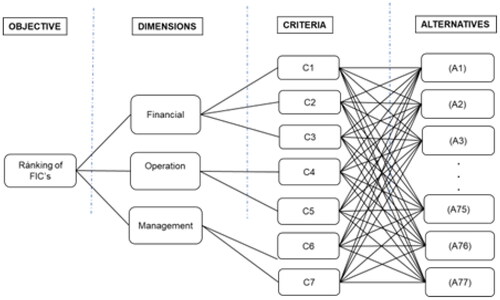
The hierarchy of the problem allows for the assimilation of a broad panorama of the problem, and how the criteria and alternatives interact.

4.7. Relative PrAToVi-B application

The literature reveals that the integration of various MCDA methods has become a standard tool, enhancing the robustness and reliability of final decision-making, regardless of the objectives for the specific problem. However, it is observed that there is often an underutilization of all available information in the generated rankings and the employment of methods that consolidate these hierarchies, which reduces the decision-maker’s uncertainty.

This innovative approach to result aggregation allows for the establishment of a unified hierarchy using another method, such as the Borda count. To determine a final ranking, it is necessary to consider alterations in the importance weights of the various criteria constituting the decision. These scenarios enable the visualization of the hierarchy’s robustness, significantly diminishing the uncertainty associated with the ranking. Each multi-criteria methodology, which is part of the same initial matrix, is shown in Table 7 (see the annexes).

Table 7. Initial decision matrix for 2021.

Dimension	Financial			Operation		Management
Criteria	(C1)	(C2)	(C3)	(C4)	(C5)	(C6)	(C7)
Indicator	Expected Value Returns	Standard Deviation Returns	Balance at Closing Date	Amount at Closing Date	Term (Days)	Credit Risk	Experience Manager
Vector	(+)	(-)	(+)	(+)	(+)	(+)	(+)
Units	%	%	Number	Number	Number	Normalized scale	Number
A1	1.63%	0.38%	278.60	219,367	268	1	11
A2	0.80%	0.23%	58.90	67	234	1	11
A5	2.69%	2.66%	897.82	9,737	279.06	0.875	11
A6	0.37%	0.34%	306.91	1,998	129	1	26
A7	0.41%	0.47%	257.40	33,134	232	1	26
A8	1.65%	0.16%	9.28	58	75	1	26
A9	1.27%	0.34%	68.59	225	129	1	26
A10	1.75%	0.16%	234.42	234	75	1	26
A11	0.95%	0.16%	126.98	8,691	75	1	26
A12	−0.36%	0.33%	186.36	11,566	212.73	1	17
A13	0.00%	0.00%	0.02	1	212.73	1	17
A14	−0.21%	0.33%	5.17	321	212.73	1	17
A15	0.05%	0.33%	0.16	10	212.73	1	17
A16	−0.21%	0.33%	116.59	7,236	212.73	1	17
A17	0.45%	0.33%	0.31	19	212.73	1	17
A18	0.81%	0.33%	0.02	1	212.73	1	17
A19	0.70%	0.37%	0.00	23	212	1	8
A20	1.11%	0.28%	5.45	36	190	1	8
A22	1.10%	0.37%	135.63	20	212	1	8
A23	−0.30%	0.35%	66.08	3,778	177.16	1	10
A24	0.19%	0.35%	0.16	9	177.16	1	10
A25	−0.94%	0.27%	5.78	36	84526	1	10
A26	−0.06%	0.27%	12.84	80	84526	1	10
A27	0.49%	0.31%	3,139.72	651,982	194841	1	12
A28	0.33%	0.36%	2.78	7	211516	1	10
A29	0.80%	0.36%	40.93	103	211516	1	10
A30	0.44%	0.36%	683.91	1,721	211516	1	10
A32	0.62%	0.49%	2.53	186	295222	1	10
A33	−0.86%	0.49%	679.09	50,011	295222	1	10
A34	−0.57%	0.49%	1.05	77	295222	1	10
A35	0.87%	0.29%	130.77	47,152	202	1	15
A36	0.87%	0.29%	40.73	14,687	202	1	15
A37	0.37%	0.23%	136.68	291	144.28	1	18
A38	0.49%	0.28%	269.08	121	269.57	1	10
A39	1.09%	0.32%	128.52	81	321.24	1	10
A40	0.39%	0.32%	4.76	3	321.24	1	10
A41	0.39%	0.32%	334.78	211	321.24	1	10
A42	0.21%	0.29%	783.32	76,558	205.95	1	15
A43	0.22%	0.29%	105.47	10,308	205.96	1	15
A44	0.34%	0.17%	259.99	75	128.02	1	15
A45	−0.08%	0.32%	72.35	107	160.32	1	19
A46	4.40%	0.84%	102.22	23	198.76	1	19
A47	0.61%	0.32%	72.35	129	160.32	1	19
A48	4.40%	0.84%	102.22	4	198.76	1	19
A49	0.45%	0.72%	10.12	223	508.22	1	19
A50	3.47%	0.84%	102.22	1,311	198.76	1	19
A51	3.07%	0.84%	102.22	12	198.76	1	19
A52	−0.15%	0.32%	72.35	80	160.32	1	19
A53	3.68%	0.84%	102.22	3	198.76	1	19
A54	0.71%	0.33%	37.71	9	155.2	1	23
A55	0.49%	0.33%	9.87	100	155.2	1	23
A56	−0.90%	1.23%	7.27	109	529.88	1	23
A57	0.67%	0.33%	8.24	96	155.2	1	23
A58	6.47%	0.10%	45.84	775	936.01	0.833	25
A59	0.20%	0.28%	4.19	453	192.48	1	25
A60	−0.30%	0.28%	2.85	308	192.48	1	25
A61	−0.25%	0.46%	3.94	21	463.89	1	25
A62	0.67%	0.29%	534.71	1,433	181.11	1	17
A63	0.71%	0.24%	208.05	171	123.24	1	10
A64	0.97%	0.29%	534.71	676	181.11	1	17
A65	1.43%	0.29%	534.71	80	181.11	1	17
A66	−0.11%	0.29%	493.71	94	199.87	1	18
A67	0.67%	0.15%	624.51	315	88.07	1	18
A68	0.67%	0.25%	51.57	2,446	169.7	1	15
A69	0.41%	0.25%	6.87	326	169.7	1	15
A70	0.87%	0.25%	0.08	4	169.7	1	15
A71	0.67%	0.25%	101.59	4,818	169.7	1	15
A72	0.19%	0.42%	52.60	1,231	273.97	1	15
A73	0.19%	0.42%	52.60	4,978	273.97	1	15
A75	0.22%	0.53%	112.27	4,606	120.25	1	6
A76	0.22%	1.23%	1.97	81	120.25	1	6
A77	1.64%	−1.01%	45.35	39	878.39	1	6

Source: Own elaboration.

In the case of PROMETHEE II, seven steps are executed to obtain the final hierarchical table. Similarly, the TOPSIS methodology concludes with a final hierarchical matrix after six steps. For the VIKOR methodology, the proposed six steps are completed to derive the final hierarchy matrix. Upon acquiring the hierarchies or rankings from these three methodologies, the Borda count is utilized to conduct the final ranking. Table 8 (see annexes) summarizes these rankings.

Table 8. Final ordering.

	Promthee II	Topsis	Vikor	Sumatoria	Ránking
A1	25	68	25	118	31
A2	57	32	55	144	24
A5	68	71	71	210	2
A6	12	15	11	38	62
A7	11	24	10	45	60
A8	8	7	3	18	69
A9	10	9	7	26	65
A10	6	5	2	13	71
A11	9	10	6	25	66
A12	45	59	50	154	18
A13	40	29	31	100	38
A14	47	55	49	151	19
A15	43	47	46	136	25
A16	44	54	48	146	22
A17	42	34	39	115	34
A18	36	20	33	89	43
A19	67	53	66	186	7
A20	64	36	61	161	14
A22	66	40	64	170	11
A23	65	63	67	195	5
A24	63	61	65	189	6
A25	56	65	57	178	10
A26	52	60	52	164	13
A27	0	17	0	17	70
A28	15	49	17	81	45
A29	14	33	14	61	54
A30	16	43	16	75	49
A32	3	38	5	46	59
A33	5	64	8	77	47
A34	7	62	9	78	46
A35	38	22	35	95	40
A36	46	23	40	109	36
A37	33	28	30	91	42
A38	60	50	60	170	12
A39	58	31	58	147	21
A40	61	56	63	180	9
A41	62	57	62	181	8
A42	41	41	38	120	30
A43	53	42	51	146	23
A44	37	30	32	99	39
A45	30	44	36	110	35
A46	20	1	12	33	64
A47	26	21	28	75	50
A48	19	2	13	34	63
A49	31	58	45	134	26
A50	23	4	20	47	57
A51	24	8	24	56	56
A52	32	48	37	117	33
A53	22	3	18	43	61
A54	1	6	1	8	72
A55	21	16	21	58	55
A56	27	67	56	150	20
A57	4	12	4	20	68
A58	2	0	22	24	67
A59	13	19	15	47	58
A60	17	37	19	73	51
A61	18	45	23	86	44
A62	35	25	34	94	41
A63	59	39	59	157	17
A64	34	14	29	77	48
A65	29	11	27	67	52
A66	39	46	41	126	28
A67	28	13	26	67	53
A68	50	27	44	121	29
A69	51	35	47	133	27
A70	48	18	42	108	37
A71	49	26	43	118	32
A72	55	52	54	161	15
A73	54	51	53	158	16
A75	69	66	68	203	4
A76	70	69	69	208	3
A77	71	70	70	211	1

Source: Own elaboration.

4.8. Stage 5: Prioritization and ranking

With the help of the MATLAB^® tool, a heatmap was established to better visualize the ranking obtained in stage 4, the result of the combination of multi-criteria methodologies, and the final ranking of the Borda count. Figure 6 shows the heatmap for the zero (0) scenario, that is, that of equal weights for the criteria.

Figure 6. Ranking of funds in the zero (0) scenario.

Source: Own elaboration.

In this map, we can identify that the funds in blue colors are ranked in the first place, that is, the best qualified and with a high probability of being selected for the portfolio; then, the funds in red colors are those in last place, which indicates their inferior performance and null selection for the portfolio. The funds that belong to the FID 17 and FID 18 SFs have a score that places them in the first five places of the classification and, therefore, many opportunities to be selected. In contrast, the funds that belong to the FID 2 trust are located last in the classification.

The results by micro category are as follows:

• Macro category: Fixed-income fund

  According to Asofiduciarias et al. (2021), these funds have portfolios exclusively invested in fixed-income instruments registered in the National Registry of Securities and Issuers (RNVE) or a world-renowned stock exchange (International Organization of Securities Commissions (IOSCO) list).

• Category: National high-yield fund

  This is the CIF with at least 50% of the value of the fund (including the available fund) invested in the fixed-income instruments described in the macro category, denominated by local currency, either from local issuers issued in the local or international market or from foreign issuers issued in the local market, and a maximum of 50% of the fund’s value in fixed-income instruments from local or foreign issuers issued in international markets denominated by foreign currency, with a maximum of 30% in foreign issuers issued in international markets denominated by foreign currency. The performance of these funds is shown in Figure 7.

  This category includes a single fund, corresponding to FID 18, and has a score that places it in any of the scenarios, first in the classification and, therefore, makes this fund a viable option to be selected.

• Category: National fixed-income fund liquidity

  This category includes fixed-income CIFs with a conservative investment policy, whose main objective is to preserve capital, with a total duration of the fund’s value of less than or equal to 240 days, and at least 80% of its portfolio invested in instruments whose national rating is greater than or equal to the second-highest rating in the long term, according to the scale used by the rating agencies in instruments with a term of more than one (1) year, whose national rating is equal to the maximum in force in the short term according to the scale used for this term in instruments with a term of less than or equal to one (1) year, or whose investments are exposed to national risk. The performance of these funds is shown in Figure 8.

  The two (2) funds that belong to the FID 18 trust have scores that place them in the first four places of the classification and therefore make them viable options to be selected. In contrast, three (3) funds that belong to the FID 2 and FID 6 trusts are in the last place of classification. The other funds in this category occupy places from the middle down.

• Category: National fixed-income fund for public entities

  CIFs with a total duration of the fund value (including available) less than or equal to 365 days, with investment policies that comply with the provisions of Decree 1525 of 2008 and its amendments and that at the request of the participating entity that manages them, are included in this category. The performance of these funds is shown in Figure 9.

  Two (2) of the funds that belong to the FID 4 trust, as well as one of the FID 5 trust funds, have a score that places them in the first 10 places of the classification and, therefore, makes them viable options for selection. One of the FID 4 funds drops considerably if Scenario eleven is presented, which gives 40% importance to the profitability criterion. In contrast, three (3) funds that belong to the FID 16 trust are located in the last place of the classification, regardless of the scenario under consideration. In the case of two (2) of the FID 5 funds, it is observed that they lose their position considerably in scenario 6 (where 50% of the weight is carried by the operation dimension), in scenario 10 (where 40% of the weight is carried by the operation dimension and 20% is carried by the value of the fund), and in scenario 15 (where 40% of the weight is carried by the criterion of the average investment term in the operation dimension).

• Category: Short-term national fixed-income fund

  This category includes the CIF for its investment objectives, maintains the total duration of the fund’s value in the range of 240 to 540 days, and at least 80% of its portfolio invested in instruments whose national rating is higher or equal to the second-highest in force in the long term according to the scale used by the rating agencies with instruments with a term of more than one (1) year; investments whose national rating is equal to the maximum in force in the short term according to the scale used for this term with instruments with a term of less than or equal to one (1) year, or investments exposed to national risk. The performance of these funds is shown in Figure 10.

  This category includes one (1) of the funds that belong to the FID 5 trust and have scores in any scenario that places them in the first five places of the classification and, therefore, makes them viable options to be selected. One of the FID 12 funds is generally located in the first quarter of the general classification but is considerably better in position if scenario 1 was presented (where 60% of the weight is carried by the financial dimension), in scenario 2 (where two financial criteria would carry 50% of the weight), and in scenario 11 (where a single criterion, risk (RI), carries 40% of the weight of the decision). Other funds constantly occupy places in the middle of the table upward, regardless of the setting, and no sudden changes or jumps are observed in the classification of this category.

• Category: Medium-term national fixed-income fund

  This category includes the CIF for its investment objectives, which maintains the total duration of the fund’s value in the range of 240 to 540 days and at least 80% of its portfolio invested in instruments whose national rating is higher or equal to the second highest in force in the long term according to the scale used by the rating agencies in instruments with a term of more than one (1) year; investments whose national rating is equal to the maximum in force in the short term according to the scale used for this term in instruments with a term of less than or equal to one (1) year; or investments exposed to national risk. The performance of these funds is shown in Figure 11.

  This category includes a single fund, corresponding to FID 13, which has a score that places it in most scenarios in the first 20 places of the classification and, therefore, makes it a medium-low option to be selected. The fund shows a considerable decrease in Scenario 7 (where 40% of the decision is carried by the management dimension and 30% of the decision is carried by the operation dimension) and in Scenario 17 (where 50% of the decision is carried by the operation dimension).

• Macro category: Exchange Traded Funds

  According to (Asofiduciarias et al., 2021), these are CIFs whose purpose is to replicate or track a national or international index, investing at least 90% of the fund in any or all of the assets in the basket comprising the index.

• Category: Beta Stock Exchange Funds

  Stock exchange-traded CIFs that exclusively replicate equity indices, at least 90% in equity investments that comprise or replicate the index. The performance of these funds is shown in Figure 12.

  This category includes a single fund, corresponding to FID 7, which has a score that places it in the bottom 25 of the ranking in most scenarios and thus makes it a medium-low option to select. The fund shows a slight rise in Scenario 17 (where 50% of the decision rests on the operation dimension).

• Macro category: Other Funds

• Category: Credit Asset Fund

  Funds whose investment policy is the acquisition of securities with credit content not registered in the RNVE through the discount modality, whose underlying is represented by invoices, promissory notes, promissory notes, among others, investing in this type of securities a minimum of 60% of the market value of its portfolio. The performance of these funds is shown in Figure 13.

  This category includes a single fund, corresponding to FID 14, which has a score that places it in the bottom of the ranking in most scenarios and thus makes it a low option to select.

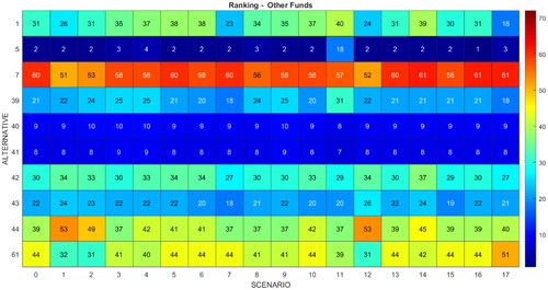
• Category: Other Funds

  Those CIFs whose investments do not fit any of the above definitions. This category shall not be subject to awards or comparisons. This category shall not be subject to awards to unitholders. The performance of these funds is shown in Figure 14.

  This category includes one (1) of the funds that belong to the FID 1 trust and have scored in any scenario that places them in the top 3 places of the classification and, therefore, make them very viable options to be selected. Two of the FID 10 funds are generally located in the top ten of the general classification in anything scenario. By the other way, the fund that belongs to FID 2 is the worst classified in this category. Other funds constantly occupy places in the middle of the table upward, regardless of the setting, and no sudden changes or jumps are observed in the classification of this category.

Figure 7. Ranking of funds in the national high-performance fund category.

Source: Own elaboration.

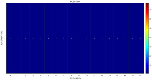
Figure 8. Ranking of funds in the national fixed-income fund liquidity category.

Source: Own elaboration.

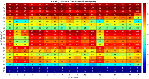
Figure 9. Ranking of funds in the national fixed-income fund public entities category.

Source: Own elaboration.

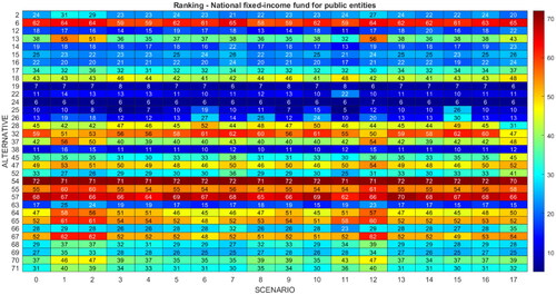
Figure 10. Ranking of funds in the short-term national fixed-income fund category.

Source: Own elaboration.

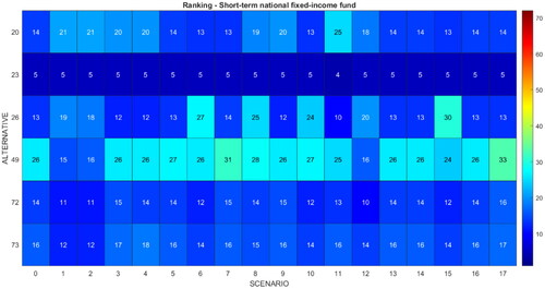
Figure 11. Ranking of funds in the medium-term national fixed-income fund category.

Source: Own elaboration.

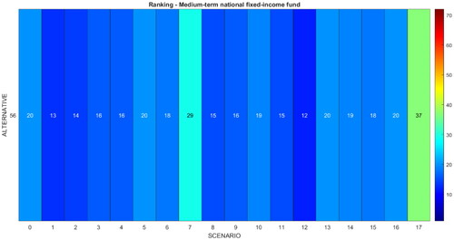
Figure 12. Ranking of funds in the Beta Stock Exchange Funds category.

Source: Own elaboration.

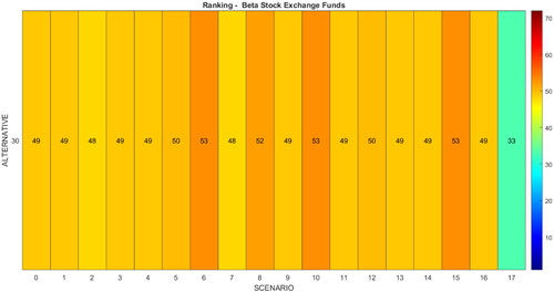
Figure 13. Ranking of funds in the Credit Asset Fund category.

Source: Own elaboration.

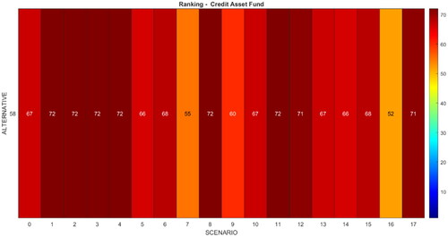
Figure 14. Ranking of funds in the other funds category.

Source: Own elaboration.

4.9. Stage 6: Scenario analysis and robustness

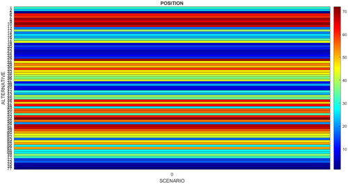
Each of the seventeen scenarios generates an ordering, that is, an interpretation of the behavior of each fund. Figure 15 summarizes the positions of each fund in each scenario and allows us to observe the performance or position of each fund.

Figure 15. Absolute ranking of funds for all categories and all scenarios.

Source: Own elaboration.

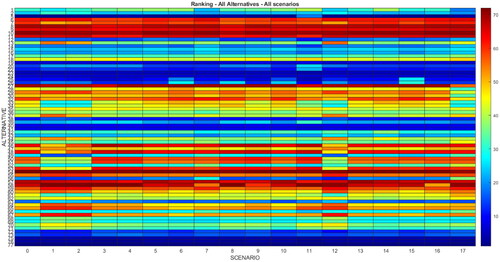
There is no significant variation in the first 10 positions between the zero (0) scenario of equal weights for all criteria and the rest of the scenarios. For scenarios one (1) to five (5), where the financial dimension carries the highest percentage, the stability of the ranking is evident. In scenarios six (6), eight (8) and ten (10), some funds of FID 4 and FID 5 that belong to the national fixed-income fund for public entities fall from the top ten positions of the other scenarios; given that, in these scenarios, the values of the criteria of the operation dimension are given greater weights, but these alternatives (funds) have low numbers of investors and short average investment terms, they are almost sight funds.

In scenario eleven (11), where each criterion is given a weight greater than 40%, the ranking is not affected by major alterations in the top twenty (20) places, even in the last twenty (20) and thirty (30) places. However, it is subtly appreciated that in scenario 12, in which the risk criterion has the greatest weight, there are considerable variations in FID 3 and FID 16 funds, which decrease significantly and belong to the national fixed-income fund for public entities category.

To strengthen the applicability and robustness of our conclusions, we have compared the data from 2022 and 2023. Tables 9 and 10 in the annexes display the initial values to be evaluated using the MCDA methodologies for 2022 and 2023, respectively.

Table 9. Initial decision matrix for 2022.

Dimension	Financial			Operation		Management
Criteria	(C1)	(C2)	(C3)	(C4)	(C5)	(C6)	(C7)
Indicador	Expected Value Returns	Standard Deviation Returns	Balance at Closing Date	Amount at Closing Date	Term (Days)	Credit Risk	Experience Manager
Vector	(+)	(–)	(+)	(+)	(+)	(+)	(+)
Units	%	%	Number	Number	Number	Normalized scale	Number
A1	4.28%	0.47%	5,129,036.09	280,653	188.14	1	12
A2	4.48%	0.47%	18,311.92	1,002	188.14	1	12
A5	7.64%	0.29%	2,644,956.36	1,127	171	0.875	22
A6	11.98%	0.56%	1,757,045.45	2,894	291	1	9
A7	10.46%	0.74%	1,134,476.98	220	245	1	26
A8	11.70%	0.33%	2,962,778.57	90	90	1	5
A9	11.98%	0.56%	138,426.53	228	291	1	9
A10	11.81%	0.33%	95,698.65	370	90	1	5
A11	10.30%	0.33%	2,867,079.91	11,085	90	1	5
A12	5.26%	0.44%	32,256.13	11,142	240	1	17
A13	0.00%	0.00%	5,790.01	2	240	1	17
A14	5.74%	0.44%	1,189,846.43	411	240	1	17
A15	6.05%	0.44%	40,530.05	14	240	1	17
A16	5.75%	0.44%	29,222.17	10,094	240	1	17
A17	6.47%	0.44%	34,740.04	12	240	1	17
A18	6.78%	0.44%	2,895.00	1	240	1	17
A19	7.04%	0.28%	1,064,860.40	2	124	1	9
A20	5.47%	0.57%	5,334.97	29	170	1	9
A22	7.35%	0.28%	1,064,860.40	23	124	1	9
A23	5.17%	0.35%	278,087.19	4,368	136.66	1	12
A24	4.28%	0.34%	38,245.31	44	96.946	1	12
A25	5.20%	0.34%	90,398.01	104	96.946	1	12
A26	5.69%	0.35%	278,087.19	8	136.66	1	12
A27	6.69%	0.34%	11,676,558.70	662,566	194	1	13
A28	6.33%	0.34%	3,153,691.12	5	173.44	1	25
A29	7.12%	0.35%	3,507,963.37	178	204	1	25
A30	−0.05%	1.46%	1,333,527.20	1,720	211	1	11
A32	6.86%	0.34%	810,559.92	119	173.44	1	25
A33	6.55%	0.34%	2,343,131.20	344	173.44	1	25
A34	5.85%	0.35%	3,507,963.37	4	204	1	25
A35	5.69%	0.31%	323,500.96	76,307	147.91	1	15
A36	5.71%	0.33%	373,073.05	88	147.91	1	15
A37	12.73%	0.53%	636,247.75	286	212.11	1	27
A38	7.08%	0.29%	1,097,829.35	127	202.592	1	12
A39	6.93%	0.34%	436,998.51	83	151.876	1	12
A40	6.17%	0.34%	21,060.17	4	151.876	1	12
A41	6.17%	0.34%	1,237,284.93	235	151.876	1	12
A42	7.05%	0.35%	3,047,210.00	76,944	111.79	1	12
A43	7.06%	0.35%	433,612.79	10,949	111.79	1	12
A44	7.49%	0.27%	1,131,560.79	87,286	93.7	1	12
A45	6.02%	0.30%	419,656.81	10,817	160	1	19
A46	6.48%	0.41%	46,847.01	2	140.49	1	19
A47	6.75%	0.30%	419,656.81	147	160	1	19
A48	6.48%	0.41%	46,847.01	2	140.49	1	19
A49	5.48%	0.86%	21,422.03	160	183.18	1	19
A50	6.48%	0.41%	46,847.01	2	140.49	1	19
A51	6.48%	0.41%	46,847.01	2	140.49	1	19
A52	6.02%	0.30%	419,656.81	125	160	1	19
A53	6.48%	0.41%	46,847.01	2	140.49	1	19
A54	5.95%	0.31%	9,627.09	6	139.4	1	29
A55	5.73%	0.31%	141,197.38	88	139.4	1	29
A56	1.83%	1.37%	17,790.72	75	516.89	1	29
A57	6.29%	0.32%	142,801.90	89	139.4	1	29
A58	8.91%	0.21%	89,369.26	486	1352.11	0.833	25
A59	5.72%	0.31%	49,558.29	448	78.8	1	25
A60	5.20%	0.31%	37,389.96	338	78.8	1	25
A61	8.57%	0.12%	93,685.11	553	1413.74	1	25
A62	14.66%	0.61%	1,540,170.73	1,323	277	1	21
A63	13.24%	0.63%	1,655,409.00	148	218	1	26
A64	14.66%	0.61%	605,358.11	520	277	1	21
A65	14.66%	0.61%	94,296.17	81	277	1	21
A66	4.88%	0.51%	971,660.53	94	152.03	1	18
A67	6.94%	0.31%	2,905,228.01	387	77.18	1	18
A68	6.88%	0.28%	14,389.50	240	95.61	1	15
A69	6.60%	0.28%	719,475.09	120	95.61	1	15
A70	7.10%	0.28%	41,969.38	7	95.61	1	15
A71	6.88%	0.28%	28,323.34	4,724	95.61	1	15
A72	5.95%	0.45%	124,758.68	1,169	171.32	1	15
A73	5.95%	0.45%	49,305.83	462	171.32	1	15
A75	6.46%	0.27%	23,255.24	5	67.18	1	7
A76	7.20%	0.27%	395,339.06	85	67.18	1	7
A77	7.20%	0.27%	79,067.81	17	67.18	1	7

Source: Own elaboration Initial decision matrix for 2022. Source: Own elaboration.

Table 10. Initial decision matrix for 2023.

Dimension	Financial			Operation		Management
Criteria	(C1)	(C2)	(C3)	(C4)	(C5)	(C6)	(C7)
Indicador	Expected Value Returns	Standard Deviation Returns	Balance at Closing Date	Amount at Closing Date	Term (Days)	Credit Risk	Experience Manager
Vector	(+)	(-)	(+)	(+)	(+)	(+)	(+)
Units	%	%	Number	Number	Number	Normalized scale	Number
A1	13.83%	0.78%	7,525,774.42	285,421	239.13	1	14
A2	14.06%	0.78%	314,166.10	11,915	239.13	1	14
A5	12.15%	0.34%	2,745,154.51	12,475	154.92	0.875	22
A6	15.46%	0.73%	2,191,601.00	2,387	203	1	9
A7	16.17%	1.00%	1,404,453.46	30,349	308	1	26
A8	14.70%	0.38%	3,128,540.00	111	94	1	5
A9	16.39%	0.73%	2,191,601.00	242	203	1	9
A10	14.78%	0.38%	123,026.31	449	94	1	5
A11	13.81%	0.38%	3,005,513.69	10,969	94	1	5
A12	14.77%	0.79%	22,937.76	7,787	209.8	1	17
A13	15.83%	0.79%	20,619.53	7	209.8	1	17
A14	15.27%	0.79%	1,402,128.12	476	209.8	1	17
A15	15.61%	0.79%	44,184.71	15	209.8	1	17
A16	15.30%	0.79%	25,633.02	8,702	209.8	1	17
A17	16.08%	0.79%	20,619.53	7	209.8	1	17
A18	16.40%	0.79%	5,891.29	2	209.8	1	17
A19	14.77%	0.65%	1,374,578.25	2	172	1	10
A20	13.52%	0.54%	5,195.67	25	146	1	10
A22	15.57%	0.65%	1,374,578.25	22	172	1	10
A23	14.46%	0.87%	321,548.84	3,274	257.83	1	12
A24	12.09%	0.80%	27,814.96	30	97	1	12
A25	13.08%	0.80%	111,259.86	120	97	1	12
A26	15.02%	0.87%	321,548.84	6	257.83	1	12
A27	15.77%	0.69%	15,527,665.04	702,670	199	1	14
A28	15.51%	0.82%	3,875,502.33	5	246.227	1	25
A29	16.81%	0.98%	4,551,348.36	174	293.513	1	25
A30	5.37%	1.02%	1,491,484.00	1,180	211	1	12
A32	16.08%	0.82%	980,455.77	127	246.227	1	25
A33	15.75%	0.82%	2,895,046.56	375	246.227	1	25
A34	15.44%	0.98%	4,551,348.36	174	293.513	1	25
A35	14.70%	0.66%	529,176.40	97	259.91	1	20
A36	14.63%	0.67%	484,105.62	89	259.91	1	20
A37	16.14%	0.80%	637,906.31	271	213.83	1	28
A38	16.40%	0.77%	1,375,136.89	189	271.531	1	13
A39	16.61%	0.87%	501,478.29	86	253.244	1	13
A40	15.73%	0.87%	17,493.43	3	253.244	1	13
A41	15.80%	0.87%	1,708,524.86	293	253.244	1	13
A42	14.30%	0.51%	4,713,714.93	98	148.63	1	12
A43	14.31%	0.51%	687,698.71	14	148.63	1	12
A44	14.61%	0.63%	745,872.99	88	156.06	1	12
A45	14.00%	0.66%	647,872.74	191	164.79	1	21
A46	15.35%	0.67%	329,414.20	2	170.96	1	21
A47	14.78%	0.66%	647,872.74	158	164.79	1	21
A48	15.35%	0.67%	329,414.20	2	170.96	1	21
A49	15.92%	0.85%	17,461.12	160	545.47	1	21
A50	15.35%	0.67%	164,707.10	2	170.96	1	21
A51	15.35%	0.67%	164,707.10	2	170.96	1	21
A52	14.00%	0.66%	647,872.74	102	164.79	1	21
A53	15.35%	0.67%	329,414.20	2	170.96	1	21
A54	14.55%	0.71%	76,614.64	13	165.86	1	17
A55	14.33%	0.71%	506,835.34	86	165.86	1	17
A56	19.25%	1.62%	21,105.76	70	429.94	1	17
A57	15.12%	0.71%	583,449.98	97	165.86	1	17
A58	12.49%	0.59%	80,589.43	376	1452.23	0.833	26
A59	14.78%	0.70%	556.82	897	263.52	1	26
A60	14.22%	0.70%	340.18	548	263.52	1	26
A61	10.33%	0.46%	66,752.24	258	1060.04	1	26
A62	12.30%	1.14%	2,811,454.18	1,431	211	1	21
A63	14.28%	0.69%	1,863,263.00	171	218	1	26
A64	12.63%	1.14%	2,470,544.32	587	211.18	1	21
A65	15.99%	0.80%	340,909.86	81	211.18	1	21
A66	14.69%	0.43%	705,658.24	87	161.9	1	18
A67	14.38%	0.96%	3,463,924.47	484	101.49	1	18
A68	15.63%	0.70%	63,926.47	2,498	199.37	1	15
A69	15.38%	0.71%	665,367.54	26	199.37	1	15
A70	16.08%	0.70%	153,546.36	6	199.37	1	15
A71	15.63%	0.70%	144,333.57	564	199.37	1	15
A72	16.83%	0.91%	43,979.53	1,141	294.73	1	15
A73	16.83%	0.90%	195,113.41	5,062	294.74	1	15
A75	16.15%	0.78%	556,218.38	6,019	267.27	1	8
A76	16.96%	0.78%	9,148.63	99	267.27	1	8
A77	16.96%	0.78%	2,217.85	24	267.27	1	8

Source: Own elaboration.

Figures 16 and 17 depict the ratings for 2022 and 2023, respectively.

Figure 16. Absolute ranking of funds in 2022 for all categories in the zero scenario.

Source: Own elaboration.

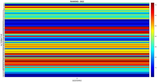
Figure 17. Absolute ranking of funds in 2023 for all categories in the zero scenario.

Source: Own elaboration.

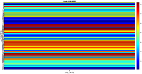
In this map, the scale is preserved in which we can identify that the funds in blue colors are ranked first, i.e. the best rated and with a high probability of being selected to form the portfolio. At the end of 2022, the funds belonging to SF FID 17 and FID 18 have, once again, a score that places them in the top five of the ranking and, therefore, a good chance of being selected. Overall, the top ten seems to remain stable, with little variation. On the other hand, the funds belonging to the FID 2 fund did show a substantial improvement. We will analyse in more detail below.

The same analysis was conducted using data from the end of the year 2023. Figure 18 presents the absolute rankings for that period.

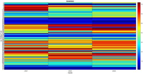
Figure 18. Comparison over three years across all categories in the zero scenario.

Source: Own elaboration.

The map consistently uses the same scale. By the close of 2023, notable shifts occur for certain funds. Specifically, SF funds FID 17 and FID 18 achieve scores that position them at the forefront of the rankings. Conversely, the funds overseen by FID 7 and FID 13 fall to the bottom ranks, diminishing their likelihood of being chosen.

The assessment encompassed three years, which were consolidated into this map. Heat maps offer the advantage of being user-friendly and intuitive for interpreting rankings. It was readily apparent that the top ten funds exhibited consistent performance across all three years. To enhance the map’s intuitiveness, we conducted further analysis, which we consider to be a reinforcement of its robustness. This analysis was grounded in Figures 19 and 20.

Figure 19. Comparison of ranking movements across three years for three categories.

Source: Own elaboration.

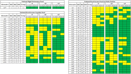
Figure 20. Comparison of ranking movements across three years for five categories.

Source: Own elaboration.

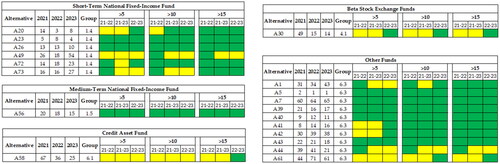
Each table displays the name of the fund categories assessed, the category code (Group), the alternatives within that category, and their rankings over the three evaluated years. The fields (21-22), (22-23), and (21-23) represent the years being compared. The fields (>5), (>10), and (>15) indicate whether the fund has ascended or descended by 5, 10, or 15 positions or more from one year to the next. The color coding is as follows: Green signifies that the change in position from one year to the next is NOT greater than 5, 10, or 15 spots, whereas yellow indicates that the change IS greater than those numbers.

For instance, Group 1.1, which pertains to the National High-Performance Fund, Alternative 17, experienced variations in its rankings that did not exceed 5, 10, or 15 positions (indicated by green boxes). This is because, from the year 2021 to 2022, it shifted by three positions, from 2021 to 2023 by four positions, and from 2022 to 2023 by just one position.

In table number 20, for group 6.1 related to the Credit Asset Fund, encompassing Alternative 58, the variations in its positions exceeded 5 and 10 positions (indicated by yellow boxes), except for the (22-23) range, which varied by eleven positions.

In general terms, we observe that the funds in the top positions show stability in the ranking over the three years, since their variations are less than fifteen positions. In terms of overall variations, we find that 27.8% of the funds (20 funds) show variations of five or less positions in the three comparisons, while 19.4% (14 funds) show variations of more than five positions. Likewise, 38.9% (28 funds) presented variations of less than ten or less positions, while 9.7% (7 funds) presented variations of more than ten positions. Finally, 61.1% of the funds (44 funds) had changes of fifteen or fewer positions and only one fund (A62) had a change of fifteen or more positions in each of the three comparisons.

5. Conclusions

Alternative investments are gaining traction, particularly in emerging nations like Colombia. Incorporating these investments into portfolios offers diversification opportunities, making it a prime time to investigate Collective Investment Funds (CIFs). Despite the information asymmetry and suboptimal structure of current CIFs, they signify a significant development in Colombia’s financial market. The classification of CIFs has enabled detailed analyses, which paves the way for further exploration of various analytical methods, such as mean-variance, semi-variance, and other risk measures in portfolio construction.

This paper integrates various aspects that address a common yet challenging financial issue: portfolio construction. This process is not merely about starting from the ground up but also includes incorporating new alternatives to diversify portfolios.

In choosing assets for portfolios, the suggested blend of mixed multi-criteria methodologies and ordinal count methods is particularly intriguing. It enables investors of any experience level to reflect their risk profile in the weights assigned to each criterion.

While multi-criteria methods are not free from subjectivity, as investors’ preferences may lean towards conservatism, the theoretical framework applied in this study lends it robustness and logical consistency. Similarly, this framework facilitates the merging of different interests or investment profiles within the same analysis, through scenario analysis and robustness, which is the measure of stability. It is crucial to note that, although traditional views suggest considering methodologies separately, this paper proposes viewing them collectively.

The comprehensive approach outlined here offers a novel perspective on decision-making by combining methods, thus potentially enriching the process by integrating other methodologies or even introducing new criteria.

Author contributions statement

All authors conceived the idea. Eduar Aguirre developed the theory and performed the computations. Dr. Pablo Manyoma and Dr. Diego Manotas verified the analytical method. Dr Manotas and Dr Manyoma encouraged Eduar Aguirre to investigate the efficient portfolio problem in CIF’s and supervise the findings of this study. All authors discussed the results and contributed to the final manuscript.

Disclosure statement

No potential conflict of interest was reported by the author(s).

Data availability statement

The authors confirm that the data supporting the findings of this study are available in the article and its supplementary materials.

Additional information

Funding

This research was self-funded by the authors and conducted during a doctoral study in Industrial Engineering at Universidad del Valle.

Notes on contributors

Eduar Fernando Aguirre González

Eduar Fernando Aguirre González, PhD candidate in Engineering at the Universidad del Valle. He also holds a Master’s degree in Engineering with emphasis in Industrial Engineering from the same university. His research interests include Financial Engineering, Financial Risk Analysis and Management, Multicriteria Decision Analysis (MCDA), Engineering and Society. He is currently a professor at Universidad del Valle and an active member of the Quantitative Finance Research Group (GIFINC).

Pablo César Manyoma Velásquez

Pablo César Manyoma Velásquez holds a PhD in Engineering on Sanitary and Environmental Engineering from Universidad del Valle in Cali, Colombia. He also has a Master’s degree in Engineering with a specialization in Industrial Engineering from the same university. His research interests include the location of unwanted service centers, Multi-Criteria Decision Analysis (MCDA), and methods and process improvement in work. Presently, he serves as a Professor at Universidad del Valle and is an active Logistics and Production Research Group member.

Diego Fernando Manotas-Duque

Diego Fernando Manotas-Duque, PhD in Engineering, Emphasis in Electric Engineering, Universidad del Valle, Cali, Colombia. Master in Administration - Emphasis in Finance, Faculty of Physical and Mathematical Sciences, University of Chile. His areas of interest are Finance, Economic Engineering, Financial Risk Analysis and Management, Financial Evaluation of Projects. Financial Management of Solidarity Economy Entities, Financial Engineering. He is currently Professor at the Universidad del Valle and director of the Quantitative Finance Research Group (GIFINC).

References

- Amin, G. S., & Kat, H. M. (2003). Hedge fund performance 1990-2000: do the ‘money machines’ really add value? The Journal of Financial and Quantitative Analysis, 38(2), 1. https://doi.org/10.2307/4126750
- Anson, M. J. P. (2002). Handbook of alternative assets. In: T. F. J. F. Series (Ed.), Portfolio the magazine of the fine arts (1st ed.). Wiley Finance. http://www.amazon.com/dp/047198020X
- Asociación de Fiduciarias de Colombia. (2013). Programa de Educación Financiera: Todo sobre Fondos de Inversión Colectiva. https://aprendiendo.baccredomatic.com/sobre/vida-financiera
- Asofiduciarias. (2021). Informe de Gestión 2021. www.asofiduciarias.org.co
- Asofiduciarias, Asobolsa, & LVAIndices. (2021). Metodología Caracterización de los FICs.
- Asofiduciarias, SIFIC, & Asobolsa. (2021). Informe Mensual FICs Categorizados-Diciembre 2021.
- Bahmani, N., Yamoah, D., Basseer, P., & Rezvani, F. (1987). Using the analytic hierarchy process to select investment in a heterogenous environment. Mathematical Modelling, 8(C), 157–30. https://doi.org/10.1016/0270-0255(87)90561-6
- Baker, H., & Filbeck, G. (2013). Alternative invesments. Instruments, performance, benchmarks and strategies (H. Baker & G. Filbeck (eds.)).
- Begué Hoyos, C. (2012). El Valor Agregado Que Ofrecen Las Inversiones Alternativas En Un Portafolio De Inversión. Escuela de Ingeniería de Antioquia.
- Black, F., & Litterman, R. (1992). Global portfolio optimization. Financial Analysts Journal, 48(5), 28–43. https://doi.org/10.2469/faj.v48.n5.28
- Bouri, A., Martel, J. M., & Chabchoub, H. (2002). A multi-criterion approach for selecting attractive portfolio. Journal of Multi-Criteria Decision Analysis, 11(4–5), 269–277. https://doi.org/10.1002/mcda.334
- Brandtner, M., Kürsten, W., & Rischau, R. (2020). Beyond expected utility: Subjective risk aversion and optimal portfolio choice under convex shortfall risk measures. European Journal of Operational Research, 285(3), 1114–1126. https://doi.org/10.1016/j.ejor.2020.02.040
- Brans, J., & De Smet, Y. (2016). Promethee methods. In Multiple criteria decision analysis (2nd ed.). Springer Science + Business Media.
- Chen, H. C., Ho, K. Y., Lu, C., & Wu, C. H. (2005). Real estate investment trusts. The Journal of Portfolio Management, 31(5), 46–54. https://doi.org/10.3905/jpm.2005.593887
- Chen, P., Baierl, G. T., & Kaplan, P. D. (2011). Venture capital and its role in strategic asset allocation. In: P. D. Kaplan (Ed.), Frontiers of modern asset allocation (1st ed.). https://doi.org/10.1002/9781119205401.ch15
- Costa, C., Bana, E., & Oliveira Soares, J. (2004). A multicriteria model for portfolio management. The European Journal of Finance, 10(3), 198–211. https://doi.org/10.1080/1351847032000113254
- Cumming, D., & Zhang, Y. (2016). Alternative investments in emerging markets: A review and new trends. Emerging Markets Review, 29(April 2015), 1–23. https://doi.org/10.1016/j.ememar.2016.08.022
- Decreto 2555. (2010). https://www.suin-juriscol.gov.co/viewDocument.asp?id=1464776
- Decreto 1242. (2013). http://www.minhacienda.gov.co/portal/page/portal/HomeMinhacienda/elministerio/NormativaMinhacienda/2013/DECRETO 1242 DE 14 DE JUNIO DE 2013.pdf
- Doumpos, M. (2018). MCDA Applications in finance. EURO PhD Summer School on MCDA/M, 79.
- Doumpos, M., & Grigoroudis, E. (2013). Applications in management and engineering. In M. Doumpos & E. Grigoroudis (Eds.), Multicriteria decision aid and artificial intelligence. Links, theory and applications (1st ed., p. 353). Jhon Wiley & Sons Ltd.
- Duque Méndez, N. D., Hernández Leal, E. J., Pérez Zapata, Á. M., Arroyave Tabares, A. F., & Espinosa, D. A. (2016). Model for the extraction, transformation and load process. Ciencia e Ingeniería Neogranadina, 26(2), 95–109. https://doi.org/10.18359/rcin.1799
- García, F., Gankova-Ivanova, T., González-Bueno, J., Oliver, J., & Tamošiūnienė, R. (2022). What is the cost of maximizing ESG performance in the portfolio selection strategy? The case of The Dow Jones Index average stocks. Entrepreneurship and Sustainability Issues, 9(4), 178–192. https://doi.org/10.9770/jesi.2022.9.4(9)
- García, F., González-Bueno, J., Guijarro, F., & Oliver, J. (2020). A multiobjective credibilistic portfolio selection model. Empirical study in the Latin American integrated market. Entrepreneurship and Sustainability Issues, 8(2), 1027–1046. https://doi.org/10.9770/jesi.2020.8.2(62)
- Hababou, M., & Martel, J. M. (1998). A multicriteria approach for selecting a portfolio manager. INFORM, 36(3), 161–176. https://doi.org/10.1016/j.jaci.2012.05.050
- Huang, X., & Ma, D. (2023). Uncertain mean-chance model for portfolio selection with multiplicative background risk. International Journal of Systems Science: Operations & Logistics, 10(1), 1–16. https://doi.org/10.1080/23302674.2022.2158443
- Hwang, C. L., & Yoon, K. (1981). Multiple attribute decision making. In Methods and Applications. (Vol. 186). Springer-Verlag.
- Kim, J. H., Kim, W. C., & Fabozzi, F. J. (2014). Recent developments in robust portfolios with a worst-case approach. Journal of Optimization Theory and Applications, 161(1), 103–121. https://doi.org/10.1007/s10957-013-0329-1
- Konno, H., & Yamazaki, H. (1991). Mean-absolute deviation portfolio optimization model and its Application To Tokyo stock market. Management Science, 37(5), 519–531. https://doi.org/10.1287/mnsc.37.5.519
- Lopez, F., & Hurtado, R. (2008). Inversiones alternativas: otras formas de gestionar la rentabilidad. Editorial especial directivos.
- Loraschi, A., & Tettamanzi, A. (2002). An evolutionary algorithm for portfolio selection in a downside risk framework. European Journal of Finance, 1, 8–12.
- Maiguashca, A. F. (2016). Una Visión de la Industria de Fondos de Inversión Colectiva en Colombia. Asofiduciarias.
- Manyoma-Velásquez, P. C. (2022). PrAToVi-B: metodología para la agregación de ordenamientos a través de análisis de decisión multicriterio robusto. Información Tecnológica, 33(4), 101–116. https://doi.org/10.4067/S0718-07642022000400101
- Markowitz, H. (1959). Portfolio selection. John Wiley & Sons.
- Opricovic, S., & Tzeng, G. H. (2004). Compromise solution by MCDM methods: A comparative analysis of VIKOR and TOP SIS. European Journal of Operational Research, 156(2), 445–455. https://doi.org/10.1016/S0377-2217(03)00020-1
- Prigent, J. L. (2007). Portfolio optimization and performance analysis. In Portfolio Optimization and Performance Analysis, Chapman and Hall/CRC Financial Mathematics Series (pp. 1–434). CRC Press, Taylor and Francis Group. https://doi.org/10.1201/9781420010930
- Rockafellar, R. T., & Uryasev, S. (2000). Optimization of conditional value-at-risk. The Journal of Risk, 2(3), 21–41. https://doi.org/10.21314/JOR.2000.038
- Romero, C. (2000). Analisis de las decisiones multicriterio (Isdefe (ed.); 1st ed., Vol. 4). http://www.sistemas.edu.bo/jorellana/ISDEFE/14 Analisis de las Desiciones Multicriterio.PDF
- Sharpe, W. F. (1964). Capital asset prices: a theory of market equilibrium under conditions of risk. The Journal of Finance, 19(3), 425–442. https://doi.org/10.1111/j.1540-6261.1964.tb02865.x
- Stephen, R. (1976). The arbitrage theory of capital asset pricing. Journal of Economic Theory, 13(3), 341–360. https://doi.org/10.1016/0022-0531(76)90046-6
- Vásquez, J. A., Escobar, J. W., & Manotas, D. F. (2021). AHP–TOPSIS methodology for stock portfolio investments. Risks, 10(1), 4. https://doi.org/10.3390/risks10010004
- Xidonas, P., Mavrotas, G., & Psarras, J. (2009). A multicriteria methodology for equity selection using financial analysis. Computers & Operations Research, 36(12), 3187–3203. https://doi.org/10.1016/j.cor.2009.02.009
- Zopounidis, C. (1999). Multicriteria decision aid in financial management. European Journal of Operational Research, 119(2), 404–415. https://doi.org/10.1016/S0377-2217(99)00142-3
- Zopounidis, C., & Doumpos, M. (2002). Multi-criteria decision aid in financial decision making: Methodologies and literature review. Journal of Multi-Criteria Decision Analysis, 11(4–5), 167–186. https://doi.org/10.1002/mcda.333