Chemometric study of some α, β-unsaturated ketone as potential antifungal agents using density function theory and GFA (ATCC 10231 and NCIM 3446 cell line)

Abstract

Quantitative structure–activity relationship (QSAR) is based on the hypothesis that changes in molecular structure reflect changes in the observed response or biological activity. The success of any QSAR model depends on the accuracy of the input data, selection of appropriate descriptors, statistical tools, and the validation of the developed model. A suitable set of molecular descriptors were calculated to represent the molecular structures of compounds such as constitutional, topological, geometrical, electrostatic, and quantum chemical descriptors. The important descriptors were selected with the aid of the genetic function approximation technique. The obtained model was validated using $R_{\text{cv}}^2$ = 0.700, LOF = 0.187, R² = 0.8085, $R_{\text{adj}}^2$ = 0.7625, F = 17.586, RMSE = 0.1781 and SDEP = 0.098, $R_{\text{pred}}^2$ = 0.7956, L_5o = 0.7235. Results showed that the predictive ability of the model was satisfactory and it can be used for designing similar group of antifungal compounds.

Keywords:

• GFA
• unsaturated ketone
• DFT
• QSAR

Public Interest Statement

Quantitative structure–activity relationship (QSAR) models are essential of the in silico techniques. They are utilized to anticipate the properties of chemicals, considering the potential harmfulness of chemicals in the body and the earth. QSAR model includes measurably examining the current information for a scope of chemicals so as to recognize precisely which structural, physical, and chemical properties of the molecule best correlate with particular measured effects on organism and the environment. QSAR models are available and in use for some end points. As a rule, QSAR models are more solid in the light of the fact that the marvel to be demonstrated is less mind-boggling and a huge number of experimental results are accessible in the information bases. Though for models to foresee endless impacts, the information are considerably more restricted and the marvel is much perplexing. It likewise helps in dissecting crude test information and confirms the test results.

1. Introduction

Fungi are widely distributed in nature and frequently appear as pathogens in the animal and plant kingdoms. The onset of the acquired immunodeficiency syndrome (AIDS) epidemic combined with increased use of immunosuppressive drugs for organ transplants and cancer therapy has resulted in increased incidence of life-threatening fungal infections (Bag, Ramar, & Degani, 2009). Chalcones are reported to have an array of important therapeutic activities such as antihypertensive, cardiovascular activity, antiprotozoal, anti-inflammatory, antidiabetic, nitric oxide inhibitory activity, anticancer activities, as well as antifungal and antitubercular activities (Bag et al., 2009). The incidence of such disease is relatively constant. Because these make infections of the skin, many of the available agents are applied topically, although a few notable oral alternatives are now available. Despite the relative triviality of the infections, however, their eradication is often problematic and requires many weeks or months of therapy (Adamuuzairu, Idris, & Bello, 2015).

The quantitative structure–activity relationship (QSAR) is an attempt, based on the structure–activity relationship (SAR) approach, to remove the element of luck from drug discovery. It uses physicochemical properties (parameters) to represent drug properties that are believed to have a major influence on the drug action. Parameters must be properties that are capable of being represented by a numerical value. These values are used to produce a general equation relating drug activity with the parameters. This equation enables medicinal chemists to predict the activity of analogs and, as a result, determine which analog is most effective to produce the desired clinical response. Its use takes some of the guess work out of deciding which analogs should be synthesized. This has the knock-on effect of reducing cost, a major consideration in all commercial companies. SAR studies are usually carried out by making minor changes to the structure of a lead to produce analogs and assessing the effect that these structural changes have on biological activity (Motta & Almeida, 2011). The success of the SAR approach to drug design depends not only on the knowledge and experience of the design team but also a great deal of luck. QSAR is an attempt to remove this element of luck from drug design by establishing a mathematical relationship in the form of an equation between biological activity and measurable physicochemical parameters (Adamuuzairu et al., 2015). Genetic function approximation (GFA) offers a new approach to building structure–activity models. It automates the search for QSAR models by combining a genetic algorithm with statistical modeling tools. Thousands of candidate models are created and tested during evolution; only the superior models survive, and are then used as “parents” for the creation of the next generation of candidate models. GFA has been successfully applied for the generation of 3D-QSAR models (Karki & Kulkarni, 2001). However, we are not always sure about the biological activities of designed novel compounds. Several experiments should be run to synthesize, and then tested to illustrate the biological impacts of the newly designed molecules. However, we are faced with time limitation and high cost of the experimental runs. Consequently, it is of interest to develop a model to predict the biological activities before any experimental works for synthesis (Pourbasheer, Aalizadeh, Ganjali, Norouzi, & Shadmanesh, 2014).

2. Materials and methods

The purpose of the present work is to perform a quantum chemical QSAR study of the ketone derivatives on the series ketone derivatives to investigate the experimental activities of the compounds as an antifungal agent and obtain a linear model using GFA techniques (Adamuuzairu et al., 2015).

2.1. Chemical data

Biological data on the activity of ketone derivatives have been obtained from Bag et al. (2009) (Tables 1 and 2). The activity data refer to pMIC, which indicates the biological activity of compounds experimentally determined, which are necessary for the inhibition of Candida albicans resistant. The –log MIC (molar) scale refers to pMIC. Their biological activity against fluconazole-sensitive as well as fluconazole-resistant strains of Candida albicans was evaluated. Tables 1 and 2 contain the biological activity for Candida albicans for α, β-unsaturated ketone.

Table 1. The main structure of unsaturated ketone (a)

	X	Y	Z	A	B	Activity (ATCC 10231) pMIC		Activity (NCIM 3446) pMIC
F	Fluconazole						F
1	F	H	H	SCH3	H	1.739	21	1.535
2	Cl	H	H	SCH3	H	1.464	22	1.163
3	Br	H	H	SCH3	H	0.923	23	0.525
4	Cl	H	Cl	SCH3	H	0.813	24	0.211
5	NO2	H	H	SCH3	H	0.780	25	0.479
6	OCH3	H	H	SCH3	H	1.457	26	1.156
7	H	H	H	SCH3	H	1.083	27	0.782
8	OH	H	H	SCH3	H	1.134	28	0.833
9	H	H	OH	SCH3	H	1.134	29	1.134
10	H	OH	H	SCH3	H	1.134	30	0.833
11	Phenyl	H	H	SCH3	H	0.522	31	0.124
12	OCH3	–	–	–	OCH3	1.199	32	1.500

Table 2. The main structure of the unsaturated ketone (b)

	X	Y	Activity (ATCC 10231) pMIC		Activity (NCIM 3446) pMIC
13		H	1.739	33	1.739
14		Br	0.946	34	0.849
15		H	1.483	35	1.182
16		Br	0.885	36	0.584
17		H	0.483	37	0.086
18		Br	0.584	38	0.186
19		H	1.111	39	1.111
20		Br	0.528	40	0.829

2.2. Computational and statistical details

QSAR studies of ketone derivatives were carried out on Windows7, Intel CORE i5 operating system by Spartan “14v112” for windows, Macintosh, and Linux. PaDEL-Descriptor (a software to calculate molecular descriptors and fingerprints), version: 2.21 and Chem3D pro, version 12.0.2 1076. The molecular structures of the data-set were sketched using Chem Draw Ultra, version 12.0.2.1076 developed by CambridgeSoft and Materials Studio V8.0.0.843 copyright(c) 2014 for the statistical analysis.

The first step consisted in obtaining the molecular geometry of all the derivatives from the data-set (Table 1) was energy minimization (Hansen, 2012) and geometry optimization using Merck Molecular Force Field (MMFF) in B3LYP/6‐311 + G(d) density functional theoretical level was used to study QSAR (Sahu, Sharma, Mourya, & Kohli, 2010).

2.3. Calculations

Molecular modeling software programs perform mathematical calculations to determine several physical and chemical properties of molecules. In general, computational chemistry programs attempt to find a solution to the Schrodinger equation, as follows:(1) $$H\mathit{\psi }=E\mathit{\psi }$$(1)

This function is an eigensystem in which the Hamiltonian operator applied to the wave function (Ψ) of the molecule is equal to an energy term (E) multiplied by the wave function, which is a mathematical expression that describes the system. The energy term in this function adjusts for the relative locations of electrons and the nucleus, and all interactions between them, while the operator is simply a function that is applied to the wave function. Once solved, the wave function can be used to calculate most properties of an atom or molecule’s geometry, behavior, or energy. However, because of the complexity of electron interactions within an atom and the increase in this complexity when atoms combine to form molecules, it is impossible to find an exact solution to the Schrodinger equation and therefore varying degrees of approximation must be applied. The computer program performs all the calculations to solve such equations, and gives the important data on the molecular system (Hango, n.d.).

2.4. Density functional theory

Density functional theory (DFT) is an ab initio approximation method for the Schrödinger equation that relies on the density or probability of electrons around a particle as a function of the radius from that particle, as opposed to wave functions as other theories employ. This theory calculates the energy of this electron density by evaluating the function, or mathematical function, of the electron density expressed as another mathematical function, meaning that it returns a number based on the electron density function. The resultant functional is partitioned into a kinetic energy term from the movement of electrons, a potential energy term from the interaction between the electrons and a positively charged nucleus in addition to the interaction between two nuclei, as well as another potential energy term from the repulsive interaction between an electron and other electrons in its vicinity. The final term describes all other electron–electron interactions that may result from various spins of electron pairs and is divided into an energy term for the same spin and mixed spin interactions. DFT is a popular method for approximation today in the computational chemistry world because it has a high accuracy per unit computer processor (CPU) time ratio in comparison to other methods (Hango, n.d.) (see Table 3).

Table 3. Parameters for energy minimization

Parameters	Value
Force field	MMFF (Merck Molecular Force Field)
Maximum no of cycles	1,00,000
Convergence criteria	0.001 cal/molǺ
Dielectric constant	1 (in a vacuum)
Gradient type	Analytical

The GFA algorithm offers a new approach to the problem of building quantitative structure–activity relationship and quantitative structure–property relationship models. Replacing regression analysis with the GFA algorithm enables the construction of models competitive with or superior to those produced by standard techniques and makes available additional information not provided by other techniques. Unlike most other analysis algorithms, GFA gives multiple models, where the populations of the models are created by evolving random initial models using a genetic algorithm. GFA can build models using not only linear polynomials but also higher order polynomials, splines, and other nonlinear functions.

The genetic algorithms are search algorithms that take inspiration from natural genetics and evolution. In this section, the ideas underlying genetic algorithms are briefly described, emphasizing the aspects relevant to the GFA approach to model building. The GFA algorithm itself applies these ideas to the problem of function approximation, given a large number of potential factors influencing a response, including several powers and other functions of the raw inputs, to find the subset of terms that correlates best with the response. The central ideas of genetic algorithms are simple. The region to be searched is coded into one or multiple strings. In the GFA, these strings are sets of terms, powers, and splines of the raw inputs. Each string represents a location in the search space. The algorithm works with a set of these strings, called a population. This population is evolved in a manner that leads it toward the objective of the search. This requires that a measure of the fitness of each string, corresponding to a model in the GFA, be available (Adamuuzairu et al., 2015).

Taking after this, three operations are performed iteratively in progression: choice, hybrid, and change. Recently added individuals are scored by wellness basis. In the GFA, the scoring criteria for models are all identified with the nature of the relapse fit to the information. The determination probabilities must be re-assessed every time another part is added to the population. Dependability and meeting in a similar manner as other iterative minimization calculations, there are issues with the steadiness and merging of the GFA calculation. A sign of the solidness of the GFA calculation can be acquired by producing a plot demonstrating the development of variable utilization with time. Such a plot demonstrates the quantity of events of every variable in the populace for every generation of the development. For commonsense reasons, to diminish the measure of information that would be gathered, such a plot is created just for those variables that happen most generally in the last populace and the information is not regularly gathered for each generation. The GFA algorithm is assumed to have converged when no improvement is seen in the score of the population over a significant length of time, either that of the best model in each population or the average of all the models in each population. When this criterion has been satisfied, no further generations are calculated.

Advantages of GFA

The GFA algorithm approach has several important advantages over other techniques.

(1)	It manufactures different models as opposed to a solitary model.
(2)	It naturally chooses which components are to be utilized as a part of the models.
(3)	It is better at finding mixes of elements that exploit relationships between numerous components.
(4)	It fuses Friedman’s lack of-fit (LOF) blunder measure, which appraises the most suitable number of components, opposes overfitting, and permits control over the smoothness of fit.
(5)	It can utilize an extensive assortment of mathematical statement term sorts in development of its models, e.g. splines, step capacities, high request polynomials.
(6)	It provides, through study of the evolving models, additional information not available from standard regression analysis, such as the preferred model length and useful partitions of the data-set. The procedure continues for a user-specified number of generations, unless convergence occurs in the interim. Convergence is triggered by lack of progress in the highest and average scores of the population.

3. Result and discussion

QSAR addresses two fundamentally important questions in scientific research; what structural and electronic properties of a molecule determine its activity and what can be altered to improve this activity? Computational tools allow researchers to identify chemicals with optimal physicochemical properties in silico, before expensive experimentation. This saves both time and money, and allows the discarding of inferior candidates well in advance of reaching the laboratory (see Table 4).

Table 4. List of descriptors used in this study

Descriptor	Type	Significance	VIF	1/VIF (Tolerance)
BCUTw-1l	BCUT	Designed to encode atomic properties that govern intermolecular interaction	1.34	0.75
PNSA-3	CPSA	Charge weighted partial negative surface area	1.18	0.85
MOMI-XZ	Moment of inertial	Is the ratio of x to y	1.93	0.52
Polar surface area	Dimensional	It combines shape and electronic information to characterize molecule	1.27	0.79
MAX ELPOT	Quantum electronics	Is a measure of energy lowering due to the maximal energy flow between donor and acceptors	1.28	0.78
Logp	Lipophilicity	The logarithm of the partition coefficient between n-octanol and water	1.32	0.76

3.1. QSAR study

To research the observed information, the dissemination of the information must be initially explored. Most relapse calculation depends on the information that is in effect regularly explored, in the event that the information is not ordinarily dispersed, we ought to think about applying as a numerical change to accomplish a typical distribution. Observed information in Table 1 showed acceptable normal distribution, so no need to perform a numerical transformation. Table 5 showed a univariate analysis for the actual data. Table 5 contains several statistical measures that describe the actual data. The most important parameters in Table 5 are the skewness and kurtosis. Skewness is the third moment of the distribution, which indicates the symmetry of the distribution.

Table 5. Univariate analysis of the observed data

		A: pMIC
1	Number of sample points	32
2	Range	1.65300000
3	Maximum	1.73900000
4	Minimum	0.08600000
5	Mean	0.88575000
6	Median	0.84100000
7	Variance	0.16562000
8	Standard deviation	0.41347700
9	Mean absolute deviation	0.32584400
10	Skewness	0.02125400
11	Kurtosis	−0.66976600

Building QSAR model is a procedure that takes an arrangement of inputs and gives an arrangement of yields. For instance, a vitality minimization is a model which takes a structure as data and gives an enhanced structure as yield. Right now in a commonplace QSAR study, count of descriptors happens. These are models which take a solitary structure as an information and give a solitary number of firmly related numbers as yields. Table 6 shows the experimental pMIC and the predicted pMIC using the GFA approach of the training set. This showed how the GFA technique predicted the pMIC.

Table 6. Experimental pMIC and GFA-predicted pMIC for the training set

	Actual values for A: pMIC	Predicted values	Residual values
1	1.46400000	1.17415500	0.28984500
2	0.92300000	1.09714100	−0.17414100
3	0.81300000	1.13876000	−0.32576000
4	0.78000000	0.62494400	0.15505600
5	1.45700000	1.59743200	−0.14043200
6	1.13400000	1.15515100	−0.02115100
7	1.13400000	1.21516000	−0.08116000
8	0.52200000	0.31406600	0.20793400
9	1.19900000	1.24385700	−0.04485700
10	0.94600000	0.99292000	−0.04692000
11	0.88500000	1.08261800	−0.19761800
12	0.48300000	0.48121300	0.00178700
13	0.58400000	0.42352200	0.16047800
14	1.11100000	0.89727600	0.21372400
15	0.82900000	0.87721400	−0.04821400
16	1.53500000	1.41141100	0.12358900
17	0.52500000	0.54215300	−0.01715300
18	0.21100000	0.18402400	0.02697600
19	0.47900000	0.41776600	0.06123400
20	1.15600000	1.17350700	−0.01750700
21	0.78200000	0.71369000	0.06831000
22	0.83300000	0.71784500	0.11515500
23	1.13400000	1.00680700	0.12719300
24	0.83300000	1.12437100	−0.29137100
25	0.12400000	0.31406600	−0.19006600
26	1.50000000	1.25590100	0.24409900
27	1.73900000	1.46277400	0.27622600
28	0.84900000	0.69688500	0.15211500
29	1.18200000	1.05402700	0.12797300
30	0.58400000	0.66801500	−0.08401500
31	0.08600000	0.40811300	−0.32211300
32	0.52800000	0.87721400	−0.34921400

Table 7 showed the GFA analysis which gives a summary of the input parameters used for the calculation. Also, it reported whether the GFA algorithm converged in the specified number of generations. Convergence is achieved when there has been no improvement in the scoring function for a number of generations. It can be seen from Table 7 that the accuracy of the model, indicated by the R² value, is reasonably high, therefore, the predictive power of the model, as indicated by the adjusted R² and cross-validated R² values, is also high, even though the regression is significant according to F-test. In Table 7, the Friedman’s LOF score (Khaled & Abdel-Shafi, 2011), which evaluates the QSAR model by considering the number of descriptors as well as the quality of fitness, is chosen: the lower the LOF, the less likely it is that GFA model will fit the data.

Table 7. Validation of the genetic function approximation

		Equation (1)
1	Friedman LOF	0.18672200
2	R^2	0.80845500
3	$R_{\text{adj}}^2$	0.76248400
4	$R_{\text{cv}}^2$	0.70000000
5	Significant regression	Yes
6	Significance of F-value	17.58623400
7	Critical SOR F-value (95%)	2.50303300
8	Lack-of-fit points	23
9	Computed experimental error	0.24950200

Use of the Friedman LOF measure has several advantages over the regular least-square error measure. In Materials Studio (Khaled & El-Sherik, 2013), LOF is measured using a slight variation in the original Friedman formula (Ameji, Uzairu, & Idris, 2015). The revised formula is:(2) $$\text{LOF}=\frac{\text{SSE}}{(1-\frac{c+dp}{M})}$$(2)

where SSE is the sum of squares of errors, c is the number of terms in the model, other than the constant term, d is a user-defined smoothing parameter, p is the total number of descriptors contained in every model term (again overlooking the steady term), and M is the quantity of tests in the preparation set. Not at all like the generally utilized slightest squares measure, the LOF measure cannot generally be decreased by adding more terms to the relapse model. While the new term may lessen the SSE, it likewise builds the estimations of c and p, which tends to expand the LOF score. Accordingly, including another term may lessen the SSE, yet really builds the LOF score. By restricting the propensity to just include more terms, the LOF measure opposes overfitting superior to the SSE measure (Khaled & Abdel-Shafi, 2011). The Friedman’s LOF score in Table 6 evaluates the QSAR model. The lower the LOF, the less likely it is that GFA model will fit the data. The significant regression is given by F-test and the higher the value the better the model (see Table 8).

Table 8. Best model

Y = −0.1052a + 0.006425b + 0.0743c − 0.07419d + 0.009784e − 0.604521f + 3.5836

Note: a = BCUTw-1l, b = PNSA-3, c = MOMI-XZ, d = polar surface area, e = max elpot and f = Logp.

3.2. QSAR model validation

3.2.1. Internal validation

The genuine convenience of QSAR models is not simply their capacity to imitate known information, confirmed by their fitting force (R²), yet basically is their potential for prescient application. Therefore, the inward consistency of the preparation set was consolidified by utilizing leave one out (LOO) cross-approval technique to guarantee the heartiness of the model (Beheshti, Pourbasheer, & Nekoei, 2012). The high calculated $Q_{\left(\text{cv}\right)}^2$ value 0.700 suggests a good internal validation. The second validation method was also developed on the basis of a leave-group-out (LGO) internal cross-validation method. In this case, a group of compounds including 20% of the training data-set were left out and predicted later by the model obtained with the remaining 80% of the data. This process was repeated five times for each one of the five unique subsets selected at random. The overall mean for this process (20% full-leave-out cross-validation), $Q_{\left(\text{L}5\text{o}\right)}^2$ = 0.7235 which indicates the robustness and stability of the constructed model (Beheshti et al., 2012).

3.2.2. External validation

If the parameters in Table 9 are subjected to equation in Table 8 using the formula below:(3) $$R^2=1-\frac{\sum (Y_{\text{pred}}-Y_{\text{obs}}{)}^2}{\sum {(Y_{\text{obs}}-{\overline{Y}}_{\text{trai}})}^2}$$(3)

Table 9. External validation of the best model (three outliers were detected i.e. compound 9, 38, and 39)

Compds	BCUTw-1l	PNSA-3	MOMI-XZ	PSA	MaxELpot	Logp	Observed Activity	Predicted Activity	Residua
1	11.998	−30.60	8.83	14.3	90.17	1.97	1.74	1.41	0.33
7	11.996	−28.35	7.68	14.3	94.45	2.25	1.08	1.21	−0.13
13	11.996	−33.81	14.88	14.7	92.03	2.57	1.74	1.46	0.28
15	11.998	−37.26	6.67	20.7	99.51	1.59	1.48	1.05	0.43
22	20.729	−60.22	0	0	0	0	1.16	1.02	0.15

The above mathematical expression yield $R_{\text{pred}}^2$ = 0.7956.

3.3. y-Randomization (y-scrambling)

This approval strategy is embraced to check models with chance connection, i.e. models where the free variables are arbitrarily connected to the reaction variables. The test is performed by computing the nature of the model (generally R² or, better, Q²) haphazardly altering the succession of the reaction vector y, i.e. by allotting to every item a reaction haphazardly chose from the genuine reactions. In the event that the first model has no chance connection, there is a huge contrast in the nature of the first model and that connected with a model got with irregular reactions. The technique is rehashed a few many times (Todeschini & Consonni, 2000). The y-randomization was carried out 10 times and it yields (RP)² = 0.6906.

3.4. Applicability domain

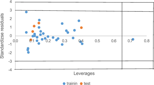
To identify chemicals that are outliers of the training set or test chemicals (Kar & Roy, 2011) that are outlying cases from the domain of applicability, both the leverages and the standardized deleted residuals are summarized in a chart called Williams plot, shown in Figure 1. Molecules in the training set are considered outlying in the X-space when their leverage exceeds the warning leverage (Beheshti et al., 2012).(4) $$h^{*}=3\frac{(K+1)}{n}$$(4)

Figure 1. The Williams plot, the plot of the standardized residuals against the leverage values.

The leverage values can be calculated for every compound and plotted against standardized residuals, and allowed a graphical detection of both the outliers and the influential chemicals in a model. Figure 1 showed the Williams plot, the applicability domain is established inside a squared (Beheshti et al., 2012) area within ± 3 bound for residuals and a leverage threshold h* (Equation 4 above), where K is the number of model parameters and n is the number of compounds in the training set. It demonstrates that all the compounds of the training set and test set are inside of this square area with the exception of one compound. From Figure 1, it is obvious that there are no outlier compounds with standard residuals >3days for both the training and test sets. Furthermore, all the chemicals have a leverage lower than the warning h* value of 0.656 except one compound and is not an outlier rather is a structurally influenced compound.

The multicollinearity between the above eight descriptors was detected by calculating their variation inflation factors (VIF), which can be calculated as follows (Beheshti et al., 2012):(5) $$\text{VIF}=\frac{1}{1-R^2}$$(5)

where R² is the correlation coefficient of the multiple regression between the variables within the model. If VIF equals to one, then no inter-correlation exists for each variable; if VIF falls into the range of 1–5, the related model is acceptable (Beheshti et al., 2012); and if VIF is larger than 10, the related model is unstable and a recheck is necessary. The corresponding VIF values of the six descriptors are presented in Table 4. As can be seen from this table, all the variables have VIF values of less than five, indicating that the obtained model has statistical significance and the descriptors were found to be reasonably orthogonal (Beheshti et al., 2012). Also for tolerance, if the tolerance is <0.20, then this would indicate that there exists multicollinearity among the descriptors. Table 4 showed that there is no significant correlation between the six selected descriptors; then, there is no multicollinearity problem on the selected subset of molecular descriptors (see Figure 2).

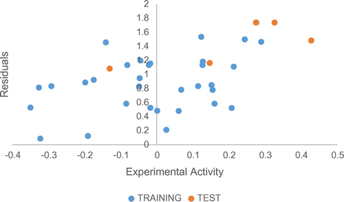
Figure 2. Relation between the predicted and observed activity using Table 6, for training and tests sets.

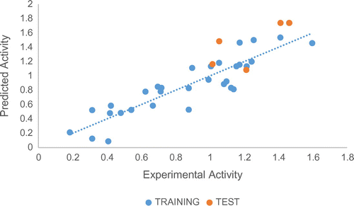
The distribution of the residual values against the observed activity values for training and test sets in Figure 3. A residual can be defined as the difference between the predicted value in the generated model and the actual measured value.

Figure 3. The residual against observed activity for the training and test sets.

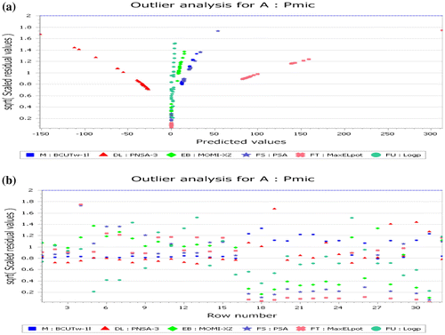
To test the constructed QSAR model, outliers analysis chart has been identified in Figure 4(a) and (b). An outlier can be defined as a data point whose residual value is not within two standard deviations of the mean of the residual values. Although the number of outliers can vary depending on the quality of the data-set (e.g. incorrect measurements of physical properties or errors in molecular structures will reduce the data-set quality), it is still a good test of QSAR model to identify potential outliers.

Figure 4(a) and (b). Outlier analysis.

Figure 4(a) and (b) contains two charts. One contains the residual values plotted against the observed pMIC and the other displays the residual values plotted against Table 1 raw number. Each chart contains a dotted line that indicates the critical threshold of two standard deviations beyond which a value may be considered to an outlier (Khaled & El-Sherik, 2013). Inspection of Figure 4(a) and (b) shows that there are no points appeared outside the dotted lines which make the QSAR model acceptable.

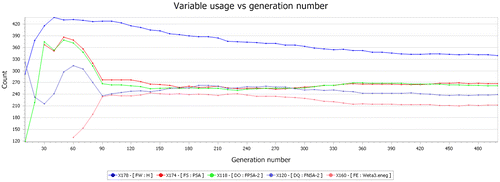
In Figure 5, the Y-axis represents the different molecular descriptors used in this study as shown on the downside of the graph. On the other hand, the X-axis represents the number of the generations we could generate for each of these molecular descriptors.

Figure 5. The graph of the variable usage against generation number.

According to Figure 5, at each step, the GFA uses the current population to create the children that make up the next generation. The algorithm selects a group of individuals in the current population, called parents, who contributed their genes, the entries of their vectors to their children. The algorithm usually selects individuals that have better fitness values as parents. User can specify the function that the algorithm uses to select the parents (Adamuuzairu et al., 2015). The GFA creates three types of children for the next generation: Elite children, crossover children, and mutation children. In our QSAR study, the algorithm stops when the number of generations reaches the value of 500 Generations.

Criteria for selection of model
N	=	number of molecule (>20 molecules)
F	=	number of descriptors in a model (statistical n/5 descriptors in a model)
Df	=	degree of freedom (n-k-1) (higher is better)
R2	=	coefficient of determination (>0.7)
Q2	=	cross-validation R2 (>0.5)
$R_{\text{pred}}^2$	=	for external test set (>0.5)
F-test	=	F-test for statistical significance of the model (higher is better for some set of compounds and descriptors). (Kar & Roy, 2011)

4. Conclusion

In this study, it was possible to obtain a multivariate QSAR model for a set of ketones that have the capability of inhibiting in vitro strain of Candida albicans. The LOO and LNO cross-validation methods, the Y-randomization technique, and the external validation indicated that the model is significant, robust, and has good internal and external predictability. The inhibitory activity of the investigated compounds was described based in descriptors: BCUT-1l, PNSA-3, MOMI-XY, POALR SURFACE AREA, MAX ELPOT, and logp properties play a significant role in explaining the activity of the data-set.

Abbreviation
GFA	=	genetic function approximation
DFT	=	density functional theory
QSAR	=	quantitative structural activity relationship
$R_{\text{cv}}^2$	=	R2 cross-validation for leave-one-out
LOF	=	lack of fit
R2	=	correlation coefficient between experimental and predicted activities
$R_{\text{adj}}^2$	=	adjusted correlation coefficient
$Q_{\text{LGO}}^2$	=	cros-validation leave-group-out
SDEP	=	standard deviation error of prediction
RMSE	=	root mean square error
F-value	=	Fischer parameter which is the significance of regression
$R_{\text{pred}}^2$	=	correlation coefficient of prediction (external)

Acknowlegdements

Mr Ajala thanks all the Lecturers of the Department for given him the opportunity to do his research computationally and creating the palatable conditions to study.

Additional information

Funding

Funding. The authors received no direct funding for this research.

Notes on contributors

Abduljelil Ajala

Abduljelil Ajala is currently an MSc student working under the supervision of Adamu Uzairu and Idris O Suleiman. Specialize on theoretical chemistry, working on modeling of organic compounds using different software and statistical tools. This research proposed a model which may provide a better understanding of the antifungal activity of ketone analogous and use as guidance for proposition of new chemopreventive agents.

References

- Adamuuzairu, A., Idris, S., & Bello, A. (2015). Qsar of ketones derivatives using genetic function approximation. IOSR Journal of Applied Chemistry, 8, 57–64. doi:10.9790/5736-08815764
- Ameji, J. P., Uzairu, A., & Idris, S. O. (2015). Quantum modeling of the toxicity of selected Anti-Candida albicans Schiff bases and their Nickel (II) complexes. Journal of Computational Methods in Molecular Design Scholars Research Library, 5, 91–103. Retrieved from http://scholarsresearchlibrary.com/archive.html
- Bag, S., Ramar, S., & Degani, M. S. (2009). Synthesis and biological evaluation of α, β-unsaturated ketone as potential antifungal agents. Medicinal Chemistry Research, 18, 309–316.10.1007/s00044-008-9128-x
- Beheshti, A., Pourbasheer, E., & Nekoei, M. (2012). QSAR modeling of antimalarial activity of urea derivatives using genetic algorithm – multiple linear regressions. Journal of Saudi Chemical Society, 1, 1–9. doi:10.1016/j.jscs.2012.07.019
- Hango, K. J. D. C. R. (n.d.). Computational chemistry (Doctoral dissertation). Worcester Polytechnic Institute.
- Hansen, K. (2012). Novel machine learning methods for computational chemistry. Berlin: Technische Universitat Berlin.
- Kar, S., & Roy, K. (2011). Development and validation of a robust QSAR model for prediction of carcinogenicity of drugs. Indian Journal of Biochemistry & Biophysics, 48, 111–122.
- Karki, R. G., & Kulkarni, V. M. (2001). Three-dimensional quantitative structure–activity relationship (3D-QSAR) of 3-aryloxazolidin-2-one antibacterials. Bioorganic and Medicinal Chemistry, 9, 3153–3160.
- Khaled, K. F., & Abdel-Shafi, N. S. (2011). Quantitative structure and activity relationship modeling study of corrosion inhibitors: Genetic function approximation and molecular dynamics simulation methods. International Journal of Electrochemical Science, 6, 4077–4094. Retrieved from www.electrochemsci.org
- Khaled, K. F., & El-Sherik, A. M. (2013). Using molecular dynamics simulations and genetic function approximation to model corrosion inhibition of iron in chloride solutions. International Journal of Electrochemical Science, 8, 10022–10043. Retrieved from www.electrochemsci.org
- Motta, L. F., & Almeida, W. P. (2011). Ketone derivatives as Anti-Candida albicans. International Journal of Drug Discovery, 3, 6–9.
- Pourbasheer, E., Aalizadeh, R., Ganjali, M. R., Norouzi, P., & Shadmanesh, J. (2014). QSAR study of ACK1 inhibitors by genetic algorithm-multiple linear regression (GA-MLR). Journal of Saudi Chemical Society, 18, 681–688. doi:10.1016/j.jscs.2014.01.010
- Sahu, N. K., Sharma, M. K., Mourya, V., & Kohli, D. V. (2010). QSAR studies of some side chain modified 7-chloro-4-aminoquinolines as antimalarial agents. Arabian Journal of Chemistry, 7, 701–707. doi:10.1016/j.arabjc.2010.12.005
- Todeschini, R., & Consonni, V. (2000). Handbook of molecular descriptors. Milano: Wiley VCH.