Ebola virus epidemic disease its modeling and stability analysis required abstain strategies

Abstract

This article discusses the Ebola virus, which is also known as Ebola haemorrhagic. Ebola virus is a transmitter virus, and the transmitting agents are wild animals, whereas in the human population it transmits from human to human. We consider the Susceptible-Exposed-Infected-Recovered (SEIR) model for our study, where the population is affected by Ebola virus by wild and domestic animals. First, we formulate the proposed model. Then, the key value, $R_0$, is obtained, which is the reproductive number of the concerned model. After that, stability analyses, both local and endemic stabilities, are carried out for disease-free equilibria and endemic equilibria and we show that both are stable. Global stability at the disease-free as well as at endemic equilibrium was found to be successfully stable. For global stability at both levels, we define the Lapnuov function, finally, numerical simulation of the Runge–Kutta method is presented for the proposed model.

Keywords:

• Ebola virus
• R₀, the reproduction number
• formulation of model
• stability resolution
• numerical interpretation

PUBLIC INTEREST STATEMENT

Microorganisms spread many diseases in both humans and animals, and then they invade each other. At present, Ebola virus is a baneful disease transmitter in urban and in some parts of rural areas. The model developed here could help in Ebola epidemiology. We propose the Ebola SEIR mathematical model, describing how the transmission of the virus spreads from both wild animals and domestic animals. The study is helpful for humans worldwide because no corner of the world is without animals. Wild animals are considered dangerous for the human society; however, this study exposed that domestic and pet animals too can prove harmful if handled without precaution. If one gets infected from Ebola virus, it well spread to the other members of the family. Thus, to avoid getting infected by Ebola virus and to realize a safe environment for human health, this study is valuable and it provides a range of precautions when handling animals.

1. Introduction

Ebola virus is one of the four ebolaviruses known to cause disease in humans. It has the highest case-fatality rate among these ebolaviruses, averaging 83% since the first outbreaks in 1976, although fatality rates up to 90% have also been recorded in one outbreak (2002–2003). There have also been more outbreaks of Ebola virus than of any other ebolavirus. In 1976, the first Ebola virus was found in “Marburg virus” (Bowen et al., 1977; Pattyn, Jacob, van der Groen, Piot, & Courteille, 1977). In the meanwhile, another team introduced the term “Ebola virus”, from Ebola River, where this river was first considered to be close to the Republic of the Congo (Bowen et al., 1977; Kuhn et al., 2010; Pattyn et al., 1977). The name “Ebola virus” is derived from the Ebola River, a river that was at first thought to be in close proximity to the area in Democratic Republic of Congo. To avoid confusion, they renamed it in 2010 as “Ebola virus”.

The incubation period, that is, the time interval from infection to the appearance of virus symptoms is 2–21 days. Humans are not infectious until they develop symptoms. The family of the related virus includes (1) Cuevavirus, (2) Marburgvirus, and also an (3) Ebolavirus. The majority of the human deaths occurred by Ebola virus, and in West Africa, it had become an epidemic from 2013 to 2015 (Na, Park, Yeom, & Song, 2016). Some cases have also been reported from West Africa; all the infected people were foreign travellers who got exposed to the virus in the affected regions and showed Ebola fever symptoms later after reaching their destinations (Reardan, 2014). During this same period, the virus caused nearly 286,16 suspected deaths and 113,10 exact and confirmed deaths (Ebola data and statistics, 2016; Ebola virus disease outbreak, 2016). The virus Ebola has spread to many countries, which started in Guinea and moved across to Liberia and Sierra Leone. The Ebola virus also spreads by human-to-human contact like secretions, blood, body fluids of the infected individuals, surfaces, and from materials used by the infected, such as cloth and bedding. The Ebola virus causes serious, acute illness and can turn fatal if left untreated.

It is believed that bats, especially fruit bats, are considered a natural pond for the Ebola virus (Quammen, 2014). The virus is transmitted from human to human and from animals to human by body fluids (Angier, 2014). In women who have been infected while breastfeeding, the virus may persist in breast milk. In health centres, healthcare workers can become infected when treating patients infected with the said disease virus. Thus, it is necessary to take great precaution. The illness is characterized by a high temperature of about 39°C, hematemesis, diarrhoea with blood, retrosternal abdominal pain, prostration with “heavy” articulations, and rapid progression to death after a mean of three days. Sore throat, headache, pain in muscle, and fever are the first symptoms of the virus. After that, the patient develops diarrhoea, vomiting, bleeding, rash, kidney pain, and some having both internal and external bleeding. The infection severity of Ebola virus can cause rapid death, or mild illness, and sometimes an asymptomatic response (Kolata, 2014). A study carried out in December 2016 showed that the vaccine of VSV-EBOV is 70–100% effective to protect against infection of the Ebola virus, which was considered the first vaccine for the said purpose (Berlinger, 2016; Henao-Restrepo et al., 2016). However, no vaccine has as yet been approved by the United States Food and Drug Administration (FDA) for use in human beings. To reduce the transmission of the virus, we need to avoid contact between infected wildlife and human beings, such as infected fruits, monkeys, and bats. Burial ceremonies that involve direct contact with the infected body of the deceased can also contribute to the transmission of Ebola. Animals should be treated with gloves, and their blood and meat should be used carefully. Similarly, the human-to-human contact with people infected with Ebola symptoms should be treated carefully and protectively, specially when handling body fluids, to reduce the chances of transmission. When an infected patient is treated at home, protective equipment should be used. After visiting the hospital or caring for patients, a regular hand wash is important. When an outbreak is detected, WHO needs to take serious steps towards the region and stop the Ebola virus from turning into an epidemic.

In this article, we will focus on Ebola virus, which has become an epidemic, like other diseases in the world. We present a model in which the disease arises from animals—both wild and domestic animals—and slowly spreads to family members, and then from them it is transferred to the hospital and care centre. Then, people who work in the centres will also get infected. This shows that this disease can become epidemic and a global problem if precautions are not used and in an unsafe treatment. We focus on the fact that if one needs to treat animals or patients infected with Ebola virus, proper precaution must be used.

2. Model formulation and method

In this article, we consider and present an Ebola mathematical model (Anderson & May, 1991; Keeling & Rohani, 2007) and we propose an Ebola SEIR virus model. In this model, the transmission of virus occurs in both ways—from both wild animals and domestic animals. We define the model in the following four classes. The first class includes the susceptible individuals, represented by $S_h$ in any time “t” who are not still infected but there might be a chance to get infected. The second class comprises exposed individuals and is represented by $E_e$, who show no symptoms of the said virus. The third class comprises $I_e$ infected individuals who were infected by Ebola virus in any period of time “t”. The fourth class of the model comprises individuals who have recovered from the Ebola virus and are represented by $R_e$. The mathematical SEIR model of the Ebola virus and its differential equations can be represented as follows:

(1) $\begin{array}{rl}& \frac{d{S}_h}{dt}=\lambda -\mu S_h-{\beta }_1{S}_h{E}_e-{\beta }_4{S}_h{E}_e-{\beta }_5{S}_h{I}_e-{\beta }_6{S}_h{E}_e-{\beta }_7{S}_h{I}_e,\\ & \frac{d{E}_e}{dt}={\beta }_1{S}_h{E}_e+{\beta }_4{S}_h{E}_e+{\beta }_6{S}_h{E}_e-{\beta }_2{E}_e{I}_e-({\mu }_1+{\mu }_2)E_e,\\ & \frac{d{I}_e}{dt}={\beta }_2{E}_e{I}_e+{\beta }_5{S}_h{I}_e+{\beta }_7{S}_h{I}_e-{\beta }_3{I}_e{R}_e-({\mu }_3+{\mu }_4)I_e,\\ & \frac{d{R}_e}{dt}={\beta }_3{I}_e-{\mu }_5{R}_e.\end{array}$(1)

With the initial conditions as

$S_h(0)\ge 0,E_e(0)\ge 0,I_e(0)\ge 0,R_e(0)\ge 0.$

We use a certain assumption in model (1), which is classified as $S_h$, which represents susceptible individuals; $E_e$ represents exposed individuals; $I_e$ represents infected individuals; $R_e$ represents recovered individuals; $\lambda$ represents a new birth rate in susceptible individuals; $\mu$ shows the natural death rate of susceptible individuals; ${\beta }_1$ indicates the rate of transmission from susceptible to exposed individuals; ${\beta }_2$ represents the transmission rate from exposed to infected individuals; ${\beta }_3$ represents the transmission rate of infected to recovered individuals; ${\beta }_4$ represents the wild animal transmission rate from susceptible to exposed individuals; ${\beta }_5$ represents the wild animal transmission rate from susceptible to infected individuals; ${\beta }_6$ represents the transmission rate of domestic animals from susceptible to exposed individuals; ${\beta }_7$ represents the transmission rate of domestic animals from susceptible to infected individuals; ${\mu }_1$ and ${\mu }_2$, respectively, represent the natural and infectious death rates of exposed individuals; ${\mu }_3$ and ${\mu }_4$ represent natural and infectious death rate of infected individuals, respectively, and ${\mu }_5$ represents the natural death rate of recovered individuals.

Since the total population is represented by the following:

$B(t)=S_h+E_e+I_e+R_e.$

which can also be written as

$\frac{dB(t)}{dt}=\frac{d{S}_h}{dt}+\frac{d{E}_e}{dt}+\frac{d{I}_e}{dt}+\frac{d{R}_e}{dt}.$

using Equation (1), we obtain the following result:

(2) $\frac{dB(t)}{dt}=\lambda -\mu S_h-({\mu }_1+{\mu }_2)E_e-{\beta }_3{I}_e{R}_e-({\mu }_3+{\mu }_4)I_e+{\beta }_3{I}_e-{\mu }_5{R}_e.$(2)

and from Equation (2), we write

$\frac{dB(t)}{dt}\le \lambda -\mu S_h.$

Clearly,

$\underset{t\to \mathrm{\infty }}{lim}supB\le \frac{\lambda }{\mu }.$

The feasible and sufficient region to study model (1) is $\mathrm{\Re }$.

$\mathrm{\Re }=\left\{(S_h,E_e,I_e,R_e)\in R_{+}^5,B\le \frac{\lambda }{\mu }\right\}.$

3. ${\mathit{R}}_{\mathbf{0}}$—The Reproduction Number

In this subsection, we determine the key value, $R_0$, which is also called the “reproductive number”, which can be defined as follows: “It is an average number whose inter in a susceptible group in the infectious period in the whole population” (Khan, Islam, Arif, & Ul Haq, 2013), and it can be calculated by the next-generation approach (Thornley, Bullen, & Roberts, 2008). The next-generation approach was presented by Driessche et al. (Van Den Driessche & Watmough, 2002) as follows:

$F=\left[\begin{array}{c}{\beta }_1{S}_h{E}_e+{\beta }_4{S}_h{E}_e+{\beta }_6{S}_h{E}_e-{\beta }_2{E}_e{I}_e\\ {\beta }_2{E}_e{I}_e+{\beta }_5{S}_h{I}_e+{\beta }_7{S}_h{I}_e-{\beta }_3{I}_e{R}_e\\ \hspace{0.17em}\end{array}\right].$

We have also,

$V=\left[\begin{array}{c}({\mu }_1+{\mu }_2)E_e\\ ({\mu }_3+{\mu }_4)\\ \hspace{0.17em}\end{array}\right].$

Now, we find $jacobian$ $\bar{F}$ and $\bar{V}$ as follows:

$\bar{F}=\left[\begin{array}{cc}{\beta }_1{S}_h+{\beta }_4{S}_h+{\beta }_6{S}_h& 0\\ 0& {\beta }_5{S}_h+{\beta }_7{S}_h-{\beta }_3{R}_e\\ \hspace{0.17em}& \hspace{0.17em}\end{array}\right].$

$\bar{V}=\left[\begin{array}{cc}{\mu }_1+{\mu }_2& 0\\ 0& {\mu }_3+{\mu }_4\\ \hspace{0.17em}& \hspace{0.17em}\end{array}\right].$

Thus, the required value of $R_0$ for the proposed model is as follows:

(3) $R_0=\frac{({\beta }_1+{\beta }_4+\beta +4)\lambda }{\mu ({\mu }_1+{\mu }_2)}.$(3)

4. Endemic equilibrium points

In this subsection, we determine the endemic equilibrium points, which play an important role in any epidemiology mathematical model. Endemic equilibrium points of the proposed model are as follows:

$S_h^{\ast }=\frac{{\mu }_5({\mu }_3+{\mu }_4)({\beta }_1+{\beta }_4+{\beta }_6)-{\mu }_5({\mu }_1+{\mu }_2)({\beta }_5+{\beta }_7)-{\beta }_3^2({\mu }_1+{\mu }_2)({\beta }_1+{\beta }_4+{\beta }_6)}{{\mu }_5({\beta }_1+{\beta }_2+{\beta }_3},$

$E_e^{\ast }=-\frac{{\beta }_2\mu +({\mu }_1+{\mu }_2)({\beta }_5+{\beta }_7)}{{\beta }_2({\beta }_1+{\beta }_4+{\beta }_6)},$

$I_e^{\ast }=\frac{-({\mu }_1+{\mu }_2)}{{\beta }_2},$

$R_e^{\ast }=\frac{-{\beta }_3({\mu }_1+{\mu }_2)}{{\mu }_5{\beta }_2}.$

5. Local behaviours of the proposed model

In this subsection, we check the stability analysis of the epidemiology system (1). Stability analysis has two sub-branches—local stability analysis at disease-free equilibrium and local stability analysis at endemic equilibrium.

6. Local behaviour of the model at disease-free equilibrium

Now the local stability analysis at disease-free equilibrium of system (1) is $D{F}_e=\left\{S_h,E_e,I_e,R_e\right\}$, which can be represented in the disease-free form as $D{F}_e=\left\{\frac{\lambda }{\mu },0,0,0\right\}$; thus, we processed the following Jacobian matrix at $D{F}_e$ as follows:

(4) $J(D{E}_e)=\left[\begin{array}{cccc}-\mu & T_1& {\beta }_5{S}_h-{\beta }_7{S}_h& 0\\ 0& T_2& 0& 0\\ 0& 0& T_3& 0\\ 0& 0& 0& T_4\\ \hspace{0.17em}& \hspace{0.17em}& \hspace{0.17em}& \hspace{0.17em}\end{array}\right].$(4)

where the terms used in the above Jacobian matrix are as follows:

$T_1=-{\beta }_1{S}_h-{\beta }_4{S}_h-{\beta }_6{S}_h,$

$T_2={\beta }_1{S}_h+{\beta }_4{S}_h+{\beta }_6{S}_h-({\mu }_1+{\mu }_2),$

$T_3={\beta }_5{S}_h+{\beta }_7{S}_h-({\mu }_3+{\mu }_4),$

$T_4=-({\beta }_5{S}_h+{\beta }_7{S}_h-({\mu }_3+{\mu }_4)){\mu }_5.$

Now, for local stability analysis at disease-free equilibrium. we have the following well-known result:

Theorem 6.1 At disease-free equilibrium $D{F}_e=\left\{\frac{\lambda }{\mu },0,0,0\right\}$ if $R_0<1$, the proposed system $(1)$ is said to be locally asymptotically stable, whereas if $R_0>1$, then we say the system (1) is unstable.

Proof: From the Jacobian matrix $J(D{E}_e)$ in equation $(4)$, we have the following eigenvalues:

(5) ${\lambda }_1=-\mu ,$(5)

(6) ${\lambda }_2={\beta }_1{S}_h+{\beta }_4{S}_h+{\beta }_6{S}_h-({\mu }_1+{\mu }_2),$(6)

(7) ${\lambda }_3={\beta }_5{S}_h+{\beta }_7{S}_h-({\mu }_3+{\mu }_4),$(7)

(8) ${\lambda }_4=-({\beta }_5{S}_h+{\beta }_7{S}_h-({\mu }_3+{\mu }_4)){\mu }_5.$(8)

At disease-free equilibrium, it is clear from Equation (5) that ${\lambda }_1=-\mu <0.$ Taking Equation (6), ${\lambda }_2=R_0-1.$ This implies that ${\lambda }_2<0$ iff $R_0<1$. Now we consider Equation (7), that is ${\lambda }_3=({\beta }_5+{\beta }_7)\lambda ÷\mu -({\mu }_3+{\mu }_4).$ Hence, its clear that ${\lambda }_3<0$ if and only if $({\beta }_5+{\beta }_7)\lambda ÷(\mu )<({\mu }_3+{\mu }_4).$ Taking Equation (8), ${\lambda }_4<0$ if and only if ${\mu }_5({\beta }_5+{\beta }_7)\lambda ÷\mu >({\mu }_3+{\mu }_4)$, which completes the proof. Hence, we can say that local stability analysis at disease-free equilibrium of system (1) is asymptotically stable.

7. Local behaviours of the model at endemic equilibrium

In this subsection, we determine the local stability analysis of the epidemiology system (1) at endemic equilibrium. For local stability analysis at endemic equilibrium, we have the following theorem.

Theorem 7.1. At endemic equilibrium, the local asymptotical stability will hold if $R_0>1$ for system $(1)$, that is, at $K{E}_e=\left\{S_h^{\ast },E_e^{\ast },I_e^{\ast },R_e^{\ast }\right\}$ and the system is unstable if $R_0>1$.

Proof: For local stability analysis at endemic equilibrium, consider the $4\times 4$ matrix

$K{E}_e=\left(\begin{array}{cccc}A& B& -({\beta }_5+{\beta }_7)S_h^{\ast }& 0\\ 0& DB-AE& -D({\beta }_5+{\beta }_7)S_h^{\ast }+A{\beta }_2{E}_e^{\ast }& 0\\ 0& B({\beta }_5+{\beta }_7)I_e^{\ast }-A{\beta }_2{I}_e^{\ast }& FA+{({\beta }_5+{\beta }_7)}^2{S}_h^{\ast }{I}_e^{\ast }& A{\beta }_3{I}_e^{\ast }\\ 0& 0& {\beta }_3& {\mu }_5\\ \hspace{0.17em}& \hspace{0.17em}& \hspace{0.17em}& \hspace{0.17em}\end{array}\right).$

After some simplification, we get the net form as follows:

$K{E}_e=\left(\begin{array}{cccc}A& B& -({\beta }_5+{\beta }_7)S_h^{\ast }& 0\\ 0& DB-AE& -D({\beta }_5+{\beta }_7)S_h^{\ast }+A{\beta }_2{E}_e^{\ast }& 0\\ 0& 0& N& -J\\ 0& 0& 0& -{\beta }_{3}J-N{\mu }_5\\ \hspace{0.17em}& \hspace{0.17em}& \hspace{0.17em}& \hspace{0.17em}\end{array}\right).$

Thus, for local stability analysis at endemic equilibrium for system (1), we get

(9) ${\lambda }_1^{\ast }=A,$(9)

(10) ${\lambda }_2^{\ast }=DB-AE,$(10)

(11) ${\lambda }_3^{\ast }=N,$(11)

(12) ${\lambda }_4^{\ast }=-{\beta }_{3}J-N{\mu }_5.$(12)

The above-mentioned terms can be specified as follows:

$A=-\mu -{\beta }_1{E}_e^{\ast }-{\beta }_4{E}_e^{\ast }-{\beta }_5{I}_e^{\ast }-{\beta }_6{E}_e^{\ast }-{\beta }_7{I}_e^{\ast },$

$B=-({\beta }_1+{\beta }_4+{\beta }_6)S_h^{\ast },$

$D=({\beta }_1+{\beta }_4+{\beta }_6)E_e^{\ast },$

$E=({\beta }_1+{\beta }_4+{\beta }_6)S_h^{\ast }-{\beta }_2{I}_e^{\ast }-({\mu }_1+{\mu }_2),$

$F={\beta }_2{E}_e^{\ast }+({\beta }_5+{\beta }_7)S_h^{\ast }-{\beta }_3{R}_e^{\ast }-({\mu }_3+{\mu }_4),$

$G=-B({\beta }_5+{\beta }_7)I_e^{\ast }-A{\beta }_2{I}_e^{\ast })(D({\beta }_5+{\beta }_7)S_h^{\ast }+A{\beta }_2{E}_e^{\ast },$

$H=(DB-AE)(FA+({\beta }_5+{\beta }_7{)}^2{S}_h^{\ast }{I}_e^{\ast },$

$J=A{\beta }_3{I}_e^{\ast }(DB-AE).$

Now we check the endemic equilibrium of system (1). Consider Equation (9) ${\lambda }_1^{\ast }=A$, which can also be written as ${\lambda }_1^{\ast }=A=-(\mu +{\beta }_1{E}_e^{\ast }+{\beta }_4{E}_e^{\ast }+{\beta }_5{I}_e^{\ast }+{\beta }_6{E}_e^{\ast }+{\beta }_7{I}_e^{\ast })$, which clearly implies that ${\lambda }_1<0$. Considered Equation (10), ${\lambda }_2^{\ast }$ which also implies ${\lambda }_2^{\ast }=DB-AE$. By placing the values and after some simplification, ${\lambda }_2^{\ast }<0$ iff $2({\mu }_1+{\mu }_2)({\beta }_5+{\beta }_7)>\mu +({\mu }_1+{\mu }_2)({\beta }_5+{\beta }_7)÷{\beta }_2({\beta }_1+{\beta }_4+{\beta }_6)S_h^{\ast }$, which is obviously greater than the second value. To verify the value of ${\lambda }_3,$ from Equation (11), we observed that ${\lambda }_3^{\ast }=N=G-H<0$ implies that ${\lambda }_3^{\ast }<0$ iff $G<H$; by performing some session of calculation, we finally obtain ${\lambda }_3<0$ if and only if $[(({\mu }_1+{\mu }_2)({\beta }_5+{\beta }_7))÷({\beta }_1+{\beta }_4+{\beta }_6)+{\beta }_3^2({\mu }_1+{\mu }_2)÷{\mu }_5]>({\beta }_5+{\beta }_7)({\mu }_3+{\mu }_4).$ Taking Equation (12) and performing some calculation, ${\lambda }_4<0$ if and only if $T>R$ and $({\mu }_1+{\mu }_2)÷{\beta }_2({\beta }_1+{\beta }_4+{\beta }_6)>{\beta }_2\mu$ and $({\mu }_1+{\mu }_2)÷{\beta }_2({\beta }_1+{\beta }_4+{\beta }_6)>({\beta }_5+{\beta }_7)({\mu }_1+{\mu }_2)$. Clearly, local stability analysis at endemic equilibrium is asymptotically stable for system (1), which completes the proof.

8. Global behaviours of the proposed model

Global stability analysis is considered one of the classical approaches in the mathematical epidemiology. So for that purpose, a special technique is developed, which is called the Lyapunov function. This approach has already been used by many authors in their works (Mwasa & Tchuenche, 2011; Thornley et al., 2008). To prove the global stability analysis of system (1), first we proved it for disease-free equilibrium and then for endemic equilibrium using the Lyapunov function.

9. Global behaviours of the model at disease-free equilibrium

To prove the global stability analysis for system (1) at disease-free equilibria, we construct a Lyapunov function for which we have the following well-known theorem.

Theorem 9.1. For global asymptotic stability, for system $(1)$ $R_0\le 1$, will hold at disease-free equilibrium if $S=S_0$ and the system is unstable for $R_0>1.$

Proof: To show global stability analysis of system (1), at disease-free equilibrium we consider the following Lyapunov function, which can be stated by the following:

$U(S_h,E_e,I_e,R_e)=\frac{1}{2}(S_h-S_h^0+E_e-E_e^0+I_e-I_e^0+R_e-R_e^0{)}^2.$

Obviously, the above-mentioned function is greater than zero at disease-free equilibrium and equal to zero at $S_h=S_h^0$ and $E_e=I_e=R_e=0$. Differentiating the above equation $U(S_h,E_e,I_e,R_e)$ with respect to $t$, and after substituting the values from system (1), we obtain the following net result:

$\frac{dU}{dt}(S_h,E_e,I_e,R_e)=(S_h-S_h^0+E_e-E_e^0+I_e-I_e^0+R_e-R_e^0)$

$(\lambda -\mu S_h-({\mu }_1+{\mu }_2)E_e-({\mu }_3+{\mu }_4)I_e-{\beta }_3{I}_e{R}_e+{\beta }_3{I}_e-{\mu }_5{R}_e.$

After simplification, we obtain

(13) $\frac{dU}{dt}(S_h,E_e,I_e,R_e)=-(S_h-S_h^0+E_e-E_e^0+I_e-I_e^0+R_e-R_e^0)(W-V).$(13)

Clearly Equation (13) is less than zero if and only if $W>V$. The terms used above are described as follows:

$W=\mu ({\mu }_3+{\mu }_4)+\frac{{({\mu }_1+{\mu }_2)}^2({\beta }_5+{\beta }_7)}{{\beta }_2({\beta }_1+{\beta }_4+{\beta }_6)}+\frac{{\beta }_3^2{({\mu }_1+{\mu }_2)}^2}{{\beta }_2^2{\mu }_5}+\frac{{\beta }_3({\mu }_1+{\mu }_2)}{{\beta }_2}.$

While

$V=\lambda +\frac{\mu ({\mu }_1+{\mu }_2)({\beta }_5+{\beta }_7)}{({\beta }_1+{\beta }_4+{\beta }_6)}+\frac{\mu {\beta }_3^2({\mu }_1+{\mu }_2)}{{\mu }_5}+\frac{\mu ({\mu }_1+{\mu }_2)}{({\beta }_1+{\beta }_4+{\beta }_6)}+\frac{{\mu }_3+{\mu }_4({\mu }_1+{\mu }_2)}{{\beta }_2}+\frac{{\beta }_3({\mu }_1+{\mu }_2)}{{\beta }_2{\mu }_5}.$

Here we observe that $\frac{dU}{dt}(S_h,E_e,I_e,R_e)=0$ if and only if $S_h=S_h^0$, $E_e=E_e^0$, $I_e=I_e^0$, and $R_e=R_e^0$, whereas $\frac{dU}{dt}(S_h,E_e,I_e,R_e)<0$ if $W>V$. Then, clearly system (1) is globally asymptotically stable at disease-free equilibrium.

10. Global behaviour of the model at endemic equilibrium

To prove the global stability analysis, we define the following Lyapunov function to verify the endemic equilibrium, and for that purpose, we have considered the following theorem.

Theorem 10.1. For global asymptotic stability for $R_0>1$, the endemic equilibrium of system $(1)$ is stable if $S_h=S_h^{\ast }$, $E_e=E_e^{\ast }$, $I_e=I_e^{\ast }$ $R_e=R_e^{\ast }$ and system (1) is unstable if $R_0<1$.

Proof: For global stability analysis at endemic equilibrium, we define the following Lyapunov function for system $(1)$:

$Q(S_h,E_e,I_e,R_e)=\frac{1}{2}(S_h-S_h^{\ast }+E_e-E_e^{\ast }+I_e-I_e^{\ast }{)}^2.$

The above-defined function $Q(S_h,E_e,I_e,R_e)>0$ and it is equal to zero at $S_h=S_h^{\ast }$, $E_e=E_e^{\ast }$, $I_e=I_e^{\ast }$ Differentiating the above equation $Q(S_h,E_e,I_e,R_e)$ with respect to “t”, we get,

$\frac{dQ}{dt}(S_h,E_e,I_e,R_e)=(S_h-S_h^{\ast }+E_e-E_e^{\ast }+I_e-I_e^{\ast })\frac{d}{dt}(S_h+E_e+I_e),$

Putting the values from system (1) in the above equation, we obtain the following:

$\frac{dQ}{dt}(S_h,E_e,I_e,R_e)=(S_h-S_h^{\ast }+E_e-E_e^{\ast }+I_e-I_e^{\ast })(\lambda -\mu S_h-({\mu }_1+{\mu }_2)E_e-{\beta }_3{I}_e{R}_e-({\mu }_3+{\mu }_4)I_e,$

Then after more simplification, finally we obtain the following result:

$\frac{dQ}{dt}(S_h,E_e,I_e,R_e)=-(S_h-S_h^{\ast }+E_e-E_e^{\ast }+I_e-I_e^{\ast })(Z-Y).$

The values of Y and Z are given as follows:

$Z=\mu ({\mu }_3+{\mu }_4)+\frac{{\beta }_3^2({\mu }_1+{\mu }_2)}{{\beta }_2^2{\mu }_5}+\frac{({\mu }_1+{\mu }_2)[({\mu }_1+{\mu }_2)({\beta }_5+{\beta }_7)-{\beta }_2\mu )]}{{\beta }_2({\beta }_1+{\beta }_4+{\beta }_6)},$

and the value of Y is also

$Y=\frac{\mu ({\mu }_1+{\mu }_2)({\beta }_5+{\beta }_7)}{({\beta }_1+{\beta }_4+{\beta }_6)}+\frac{\mu {\beta }_3^2({\mu }_1+{\mu }_2)}{{\mu }_5}+\frac{({\mu }_3+{\mu }_4)({\mu }_1+{\mu }_2)}{{\beta }_2}.$

Hence, we have $\frac{dQ}{dt}(S_h,E_e,I_e,R_e)=0$ if and only if $S=S_h^{\ast }$, $E_e=E_e^{\ast }$, $I_e=I_e^{\ast }$, and $R_e=R_e^{\ast }$; also $\frac{dQ}{dt}(S_h,E_e,I_e,R_e)<0$ if $Z>Y$ Y; from this, it is clear that system (1) is globally asymptotically stable at endemic equilibrium, which completes the proof.

11. Numerical simulation and discussion

This subsection contains numerical interpretation of system (1) using the Runge–Kutta method. Different parameters, their values, and their numerical results are stated in Figures 1–4, all without vaccination, whereas Figures 5–6 present both with and without vaccination. For this purpose, we present the following table.

Table

Notation	Description of Parameter	Value
$\lambda$	New birth rate in susceptible individuals	$0.6321$
${\beta }_1$	Transmission rate from susceptible to exposed individuals	$0.2877$
${\beta }_2$	Transmission rate from exposed to infected individuals	$0.7613$
${\beta }_3$	Transmission rate from infected to recovered individuals	$0.4389$
${\beta }_4$	Individuals get wild animals’ infection from susceptible to exposed	$0.1234$
${\beta }_5$	Individuals get wild animals’ infection from susceptible to infected	$0.2431$
${\beta }_6$	Individuals get domestic animals’ infection from susceptible to exposed	$0.4000$
${\beta }_7$	Individuals get domestic animals’ infection from susceptible to infected	$0.3000$
$\mu$	Natural death rate of susceptible individuals	$0.9704$
${\mu }_1$	Natural death rate of exposed individuals	$0.0432$
${\mu }_2$	Infectious death rate of exposed individuals	$0.2006$
${\mu }_3$	Natural death rate of infected individuals	$0.0656$
${\mu }_4$	Infectious death rate of infected individuals	$0.9764$
${\mu }_5$	Natural death rate of recovered individuals	$0.6704$

Figure 1. Plot showing the population of susceptible individuals.

Figure 2. Plot showing the population of exposed individuals having Ebola virus.

Figure 3. Plot showing the population of infected individuals having Ebola virus.

Figure 4. Plot showing the population of recovered individuals having Ebola virus.

Figure 5. Plot showing the population of susceptible individuals with and without control of Ebola virus.

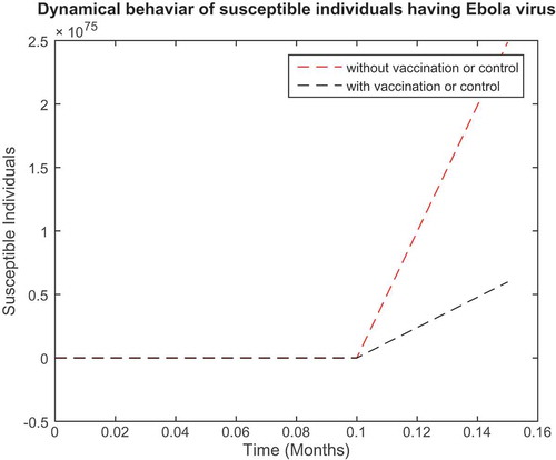
Figure 6. Plot showing the population of exposed individuals with and without control of Ebola virus.

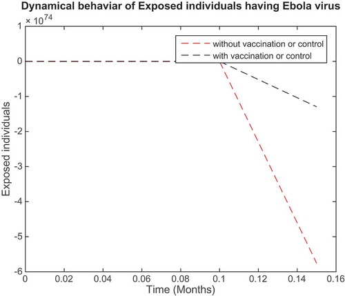
All values were considered as fixed in the above table. In Figures 1–4, simulations are presented without vaccine, whereas Figures 5–8 presented both with and without control or vaccine (Mwasa & Tchuenche, 2011). Figure 1 shows that the graph for susceptible individuals is initially high, but after some time, it starts decreasing. Figure 2 shows that the exposed individuals initially show no symptoms of virus, but after some time they show symptom of Ebola virus and gradually increase. In Figure 3, the graph for the infected individuals is initially high, but with time, it gradually decreases. In Figure 4, the simulation is initially high, but then the recovered individuals get well after some time and then tend to zero. Next graph 5 is presented with and with out vaccine; initially, graph 5 is high without vaccination, but with vaccine it decreases in intensity. Figures 6 and 7 show the same behaviour, and with vaccine it decreases to zero rapidly. We see in Figure 8 that the recovered people feel well after some time after getting vaccinated.

Figure 7. Plot showing the population of infected individuals with and without control of Ebola virus.

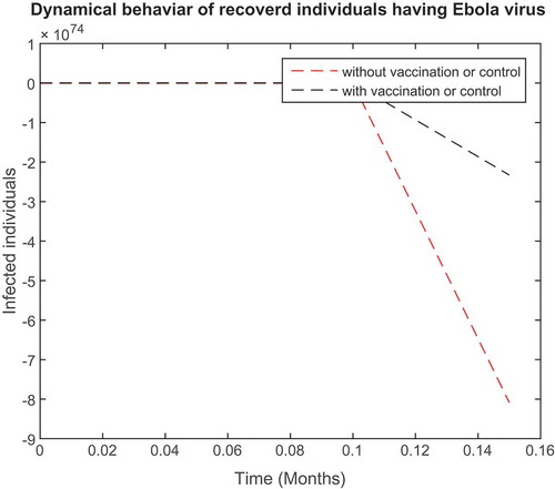
Figure 8. Plot showing the population of recovered individuals with and without control of Ebola virus.

12. Conclusion about the proposed model

A compartmental (SEIR) epidemic model of the Ebola virus was considered. In our proposed model two new issues were drawn—one for wild animals and the other for domestic animals, which spreads infection in the population at any time “t”. In the first step, we formulated the model, and we obtained the basic reproductive number, $R_0$. Then, we calculated the endemic equilibrium points. After that, local stability and global stability at disease-free equilibrium were obtained and were found to be stable for system (1), $R_0=1$. Furthermore, local and global stabilities at endemic equilibrium were found to be stable, and this showed that the endemic equilibrium is locally as well as globally asymptotically stable for $R_0>1$ with the help of the Lyapunov function. Finally, we obtained the numerical solution of the compartmental mathematical model using the Runge–Kutta method RK4 tool, and we presented the results in Figures 1–4 without vaccination and in Figures 5–8 both with and without vaccination.

Competing interests

The authors declare no competing interests.

Acknowledgements

All authors equally contributed to this paper.

Additional information

Funding

The authors received no direct funding for this research.

Notes on contributors

Muhammad Tahir

Muhammad Tahir is the corresponding author of this research article and his research areas include mainly mathematical biology, microorganisms virus diseases, fluid mechanics, and fluid dynamics. He is a PhD research scholar at the Department of Mathematics, Islamia College University Peshawar, Pakistan, a public sector university. His e-mail address is [email protected] and his telephone number is [phone].

Syed Inayat Ali Shah

Syed Inayat Ali Shah is currently working as a professor and dean in Mathematics at Islamia College University, Peshawar, Pakistan. He obtained his PhD degree from Saga University Japan in 2002. He has published various peer-reviewed articles and has submitted a number of papers for peer review. His e-mail address is [email protected]

Gul Zaman

Gul Zaman is currently a Vice Chancellor at University of Malakand Pakistan. He has published a number of peer-reviewed articles in the areas of mathematical biology, fluid mechanics, and fluid dynamics. He has done his PhD from the Department of Mathematics, Pusan National University, Pusan, South Korea, with the dissertation titled “Blood Flow of Oldroyd-B Type Fluids Induced by Brownian Force in a Vessel”. He is also the HEC (Pakistan)-approved supervisor and has performed some approved projects. His e-mail address is [email protected]

Sher Muhammad

Sher Muhammad is working in Cecos University of IT and Emerging Sciences Peshawar, Pakistan, as lecturer in Mathematics. Moreover, he is a PhD research scholar at the Department of Mathematics, Islamia College University Peshawar, Pakistan, a public sector university, and his field of interest is mathematical biology, fluid mechanics, and fluid dynamics. His e-mail address is [email protected]

References

- Anderson, R. M., & May, R. M. (1991). Infectious diseases of humans: Dyn and cont. Oxford, UK: Oxford University Press.
- Angier, N. (2014, October 27). Killers in a cell but on the loose Ebola and the vast viral universe. New York Times.
- Berlinger, J. (2016, December 22). Ebola vaccine gives 100 percent protection, study finds. CNN. Retrieved 27 December 2016.
- Bowen, E. T. W., Lloyd, G., Harris, W. J., Platt, G. S., Baskerville, A., & Vella, E. E. (1977). Viral haemorrhagic fever in southern Sudan and northern Zaire. Preliminary studies on the aetiological agent. Lancet, 309(8011), 571–573. PMID 65662. doi:10.1016/s0140-6736(77)92001-3
- Ebola data and statistics. (2016). World Health Organisation. Retrieved June 9.
- Ebola virus disease outbreak. (2016). World Health Organization. Retrieved December 4.
- Henao-Restrepo, A. M. et al. (2016, December 22). Efficacy and effectiveness of an rVSV-vectored vaccine in preventing Ebola virus disease: Final results from the Guinea ring vaccination, open-label, cluster-randomised trial (Ebola Ça Suffit!). The Lancet, 389(10068), 505–518. PMC 5364328?Freely accessible. PMID 28017403. doi:10.1016/S0140-6736(16)32621-6
- Keeling, M., & Rohani, P. (2007). Modelling infectious diseases in humans and animals. Princeton, NJ: Princeton University Press.
- Khan, M. A., Islam, S., Arif, M., & Ul Haq, Z. (2013). Transmission model of hepatitis B virus with the migration effect. Hindawi Publishing Corporation BioMed Research International, 150681, 10.
- Kolata, G. (2014, October 30). Genes influence how mice react to Ebola, Study Says in ’Significant Advance’. New York Times.
- Kuhn, J. H., Becker, S., Ebihara, H., Geisbert, T. W., Johnson, K. M., Kawaoka, Y., … Negredo, A. I., et al. (2010). Proposal for a revised taxonomy of the family Filoviridae: Classification, names of taxa and viruses, and virus abbreviations. Archives of Virology, 155(12), 2083–2103. PMC 3074192?Freely accessible. PMID 21046175. doi:10.1007/s00705-010-0814-x
- Mwasa, A., & Tchuenche, J. M. (2011). Mathematical analysis of a cholera model with public health interventions. BioSystems, 105(3), 190–200. doi:10.1016/j.biosystems.2011.04.001
- Na, W., Park, N., Yeom, M., & Song, D. (2016, December 4). Ebola outbreak in Western Africa 2014: What is going on with Ebola virus? Clinical and Experimental Vaccine Research, 4(1), 17–22. ISSN 2287-3651. PMC 4313106?Freely accessible. PMID 25648530. doi:10.7774/cevr.2015.4.1.17
- Pattyn, S., Jacob, W., van der Groen, G., Piot, P., & Courteille, G. (1977). Isolation of Marburg-like virus from a case of haemorrhagic fever in Zaire. Lancet, 309(8011), 573–574. PMID 65663. doi:10.1016/s0140-6736(77)92002-5
- Quammen, D. (2014, December 30). Insect-eating bat may be origin of Ebola outbreak, new study suggests. news.nationalgeographic.com. Washington, DC: National Geographic Society.
- Reardan, S. (2014). The first nine months of the epidemic and projection, Ebola virus disease in west Africa. archive of Ebola Response Team. New England Journal of Medicine, 511(75.11), 520.
- Thornley, S., Bullen, C., & Roberts, M. (2008). Hepatitis B in a high prevalence New Zealand Population a mathematical model applied to infection control policy. Journal Theoretical Biologic, 254, 599–603. doi:10.1016/j.jtbi.2008.06.022
- Van Den Driessche, P., & Watmough, J. (2002). Reproduction numbers and sub threshold endemic equilibria for compartmental models of disease transmission. Mathematical Biosciences, 180, 29–48. doi:10.1016/S0025-5564(02)00108-6