Are prices of New dwellings different? A spectral analysis of UK property vintages

Abstract

The work makes two contributions to the literature on dynamic house prices. First, a house price ripple in cycles from Modern to Older dwellings is revealed and, second, as New housing is shown to have lower volatility than the other two. Using spectral analysis, it is argued that there is a 7½-year repeat buyer-second-hand cycle and a five year, first time buyer-New housing cycle, common to three house price vintages. These cycles reinforce each other every 15 years, which corresponds with a Minsky super-cycle in housing finance. The equity of the owner–occupier is fortified by higher house prices whereas New builds extract embedded equity from the market. Through programmes like Help-to-Buy 1, Government should support builders and facilitate market access to FTBs. However, to address the greater price instability that should follow, Government should impose a capital gains tax on the house seller.

Keywords:

• spectral analysis
• UK house prices
• housing vintages

Public Interest Statement

The repeat buyer is the driver behind a 7.5-year cycle in UK house prices, whereas the first-time buyer is more closely linked to the shorter cycle. These two cycles, evident in construction expenditure and house prices, would reinforce each other every 15 years, reflecting perhaps a Minsky super-cycle of that order in housing finance.

A recent policy initiative in the UK, the Help-to-Buy 1 scheme, seeks to support first-time buyers and the construction of New housing. Both of these should reduce price volatility in the market. Help-to-Buy 2, which supports all vintages and all buyers, would fortify the market power of the repeat buyer, which should increase price volatility and hinder affordability. For greater price stability, Government should impose a capital gains tax on the house seller.

1. Introduction

Numerous authors have analysed the codynamics of stratified housing markets. Hui (2011) classifies various threads of literature into three groups. First, the ripple effect is where house price increases in the UK appear to be led by London and the South East (inter alia Gray, 2012; Meen, 1999). Second, there is price diffusion among housing of differing qualities (Coulson & Mcmillen, 2007; Ho, Ma, & Haurin, 2008; Hui, 2011; Smith & Ho, 1996). Building on a model due to Stein (1995), Mayer (1993) argues it is not necessarily quality but price that matter; high-priced homes are sensitive to low-priced ones. The third relates to distinct house price dynamics among differing sub-markets (Renaud, Zhang, & Koeberle, 1998); some housing markets behave in an idiosyncratic manner. An example, Cook and Holly (2000), consider three housing vintages. One could argue that an additional fourth strand would entail considering a ripple through these differing housing vintages if such relationships should be found.

New and second-hand housings serve the same function but have slightly differing characteristics. New builds will be constructed with the benefit of contemporary techniques and technologies and are likely to come with a warrantee implying that, for a representative property, the price should be higher. Barras and Ferguson (1985) suggest that property vintages will depreciate at approximately the same rate. As such, there should be a stable ranking of prices for a representative house from each vintage.

Stein (1995) and Ortalo-Magne and Rady (2006) argue that embedded equity in credit-constrained repeat buyers’ (RBs’) properties fuel house price volatility. Ownership in a period of rising prices extends to the vendor of a windfall gain that can be used to trade-up or be withdrawn as capital. Neither contribution focuses on the vintage of properties, nor on the buyer that has a property to sell. A key distinction among vintages is that New housing will not have this windfall embedded in the price. Rather, the increase in the supply of New housing will depress the value of embedded equity in second-hand dwellings. This implies that the dynamics of New will be distinct from second-hand house prices. Using New, Modern and Older house prices data from the UK, this paper considers: firstly, whether second-hand housing has greater price volatility; and secondly, whether it has distinctive dynamics compared with New dwellings.

The paper is structured as follows. First, models of house price volatility and credit constraints due to Stein and Ortalo-Magne and Rady are discussed. Next, relevant literature on the cyclical nature of property is considered. The data and methodology, spectral methods, are discussed next followed by an analysis of results. As substitutes, New and second-hand house price dynamics could be characterised by common trends and cycles in a cointegration sense. What is found is that, consistent with Renaud et al., and Cook and Holly, there are distinctions in the dynamics of New relative to Modern and Older house prices, most clearly revealed at a five and a half year cycle: second-hand prices are more volatile than New.

Private dwelling construction expenditure is used as an indicator of supply conditions. It is likely that credit conditions are reflected in both price and construction expenditure. It is possible that the combination of a five and a seven and a half-year cycle would generate a super-cycle of 15 years, which appears to colour housing indicators and is in line with Minsky’s work on bubbles, where financial liberalisation is a driver of asset prices.

2. House price volatility

Stein and Ortalo-Magne and Rady consider the role of credit in the determination of house prices. Stein’s model has only owner–occupiers whilst Ortalo-Magne and Rady allow for non-home ownership to begin with. Both presume a fixed supply of housing. Ortalo-Magne and Rady concentrate on: a (short) housing ladder and a life cycle; two classes of buyer—the first-time buyer (FTB) and the RBs; and the down payments on a “starter” home typified as a “flat” and the “trade up” home typified as a “house”. Credit-constrained, owner–occupiers acquire more expensive “houses”, in the main. A “house” owner may extract embedded equity by trading down to a “flat” in the last phase of their life cycle.

For Stein and Ortalo-Magne and Rady, credit-constrained buyers exploiting embedded equity in their property fuel house price instability. For Stein, as higher prices relax the budget constraint on owners, demand for property increases with price. Ortalo-Magne and Rady suggest something similar.

Getting on the housing ladder is vital for the FTB. By buying earlier, it is the capital gain that allows the credit-constrained smaller/cheaper “flat” owner to trade-up to a more expensive/larger “house”. With an identical percentage increase in income and price, the absolute gap between the two expands, at some point shifting the “flat” from “within means” to unaffordable. Moreover, the FTB has a dual effect. First, they supply the capital for the current “flat” owner’s to inject into the “house” they seek to acquire. Second, when they participate in the market, the FTB boosts demand for cheaper “flats”.

2.1. Market participation

The mix of FTBs and RBs in the market changes with house price inflation. With increasing prices, a decreasing number of FTBs can supplement the mortgage loan with their own savings to purchase a property. Concurrently, the greater equity in the owner–occupier’s property encourages speculative sales and purchases. More FTBs see their price maximum breached whilst, as their “reservation” prices are passed, RBs swell the market, comprising a higher proportion of buyers. Because embedded equity is a positive function of price, the demand curve for housing could be upward sloping (Dusansky & Wilson, 1993) for some portion. As they are priced in rather than out, RBs’ market participation lasts longer than for FTBs.

FTB participation may be driven by life events, such as starting a family, over which they may be some, but relatively little discretion over timing. By contrast, the ability of owners of second-hand dwellings to withdraw their properties from the market in a downturn or offer them in an upturn at little time or cost constraint adds turnover volatility to the markets when prices are already changing rapidly.

Current house hunters will be better placed to know the present state of prices, so non-participant RBs with second-hand properties that are subsequently induced onto the market by higher prices are so with a time lag. As FTBs are priced out of the market, RBs increasingly trade second-hand dwellings with each other in a febrile atmosphere. The FTB cycle could have a lower peak and a shorter periodicity compared with the RBs.

2.2. A property focus

Shifting the focus from the owner to the property, it is proposed that, as it will not contain a windfall embedded in the price, New housing has a different effect on market volatility compared with second-hand dwellings that are put up for sale by RBs. A rise in price will fortify the “flat” owner’s purchasing power. As they trade-up and buy a second-hand “house”, this embedded windfall will be transferred to an existing owner, enhancing their potential market leverage.

New dwellings capture for the builder the capital that would otherwise be transferred to another home-owner. In other words, a New property extracts the capital gain that the second-hand property owner uses to trade-up. As they will reduce the embedded capital gain in the system, the release of New “houses” and “flats” should disinflate second-hand price dynamics doubly: an increase in supply will lower price pressures; and the sale of a New property will withdraw equity from the second-hand market, reducing price volatility. The builder will have less discretion about property supply than the RB. They may be able to accelerate work in progress as prices to rise and drip feed in the decline. However, the builder may need the embedded equity to move on to the next project (Stein, 1995).

From the above discussion, it is averred that temporal variations in the numbers of FTBs and New properties in the market will be lower than RBs and second-hand dwellings. As both builders and buyers are dependent on bank finance, they are likely to be codriven by a third factor, credit. Thus, construction expenditure could lead prices without [Granger] causing them. Given that New and second-hand housing are substitutes, demand-driven price changes should affect both contemporaneously.

Decisions to build and sell will be based on price expectations. Meen (1996) suggests that, as they represent accumulated equity that can be used to ascend the housing ladder, lagged house prices influence current ones. Maclennan, Muellbauer, and Stephens (1998) argue that the history of house prices influences future prices. If consumers experience heavily autocorrelated house prices, they will build that into their expectations, tending to make history repeat itself. One of DiPasquale and Wheaton’s (1996) models of house prices, based on myopic price expectations, predicts that a demand shock stimulates construction and the expectation of further price rises. Rising price reinforces the view that they will climb further. Financiers, when flushed with money and holding the same myopic view, loosen lending criteria to keep buyers in the market. This process, as analysed by Minsky, can be seen in other asset markets. Palley (2011) explains that Minsky postulates two cycles; a basic and a super-cycle. Agents become progressively more optimistic about future prices, taking on more risk. There is a relaxation of credit constraints and increased prices. Borrowers initially can afford the interest and capital repayments. The next phase involves just meeting the interest payments on the capital, and the cycle ends with the borrower relying on capital gains to meet their obligations, which may force them to sell. In housing, it is averred that it is unaffordability coinciding with the increased supply of New housing that bursts property bubbles (Bover, Muellbauer, & Murphy, 1989; DiPasquale & Wheaton, 1996; Pyhrr, Roulac, & Born, 1999). The downturn in the cycle occurs when there is excess supply altering price expectations. However, Minsky’s analysis would suggest that excess supply of New housing need not be the source of the turning point; the unserviceability of loans would be sufficient.

Minksy’s super-cycle entails an erosion of the structures and institutions that moderate lending. With housing, this would be seen in a relaxation of lending criteria such as loan-to-value (LTV) and loan-to-income (LTI) ratios. Switching buyers to interest only mortgages without a repayment vehicle; self-certified mortgages where the borrower reported an income which the lender took on faith; and offering mortgages of a LTV of over 100% featured as less than prudent lending practices in the 2000s. Palley (2010) observes a 30-year super-cycle in the USA involving financial innovation, financial deregulation and changed investor attitudes to risk. This overarches three business cycles (1981–1990, 1991–2001 and 2002–2009), each of which was “marked” by a basic cycle in which borrowers and lenders took on increasingly more financial risk.

3. Evidence of cycles in property

Property is an asset class where periods of under- and oversupply are the norm (DiPasquale & Wheaton, 1996; Pyhrr et al., 1999). Using univariate spectral analysis, common cycles among stock indices of the property sector in Singapore, Hong Kong, Malaysia, Japan and the UK of about 2½–4 years are exposed by Liow (2007). Chen, Kawaguchi, and Patel (2004) reveal two or three hidden periodicities in house price series from Hong Kong, Singapore, Taipei and Tokyo from 1976 to 1998. They find a business cycle (of around 7.9–10.4-years), an intermediate cycle (3.2–4.4 years) and an annual cycle. They depict the business cycle as driven by exogenous shocks and the four-year periodicity as an endogenous, production lag cycle. Alexander and Barrow (1994) and Rosenthal (1986) find, in UK regional house prices, a five- to ten- and six- to eight-year periodicity, respectively. Wilson and Okunev (1999) reveal high cospectra values between real estate investment trusts and financial assets markets at cycles of 3 years in Australia, 3½ in the USA, and 6 and 8 years in UK series.

Barras and Ferguson (1985) find a major cycle of 6½ years for New orders for private housing construction in UK data, which can be distinguished from a second, shorter 3¾-year cycle. Construction of New housing exhibits a single cycle of 21 quarters.

Benito (2006) find the UK housing market has characteristics consistent with Ortalo-Magne and Rady and Stein. There is greater volatility for former owner–occupiers’ house price inflation than for FTBs; the proportion of RBs increases with inflation; and prices are sensitive to the incomes of the young.

Cook and Holly (2000) consider whether there are common trends and cycles among Older, Modern and New UK house prices. New housing is not cointegrated with second-hand housing on a pairwise basis. Non-synchronised, common cycles are found among the three series. This is interpreted as differential reactions to a common shock. They do not consider a ripple effect in these cycles. They find that New housing is more volatile, showing a tendency to rise more rapidly and to higher peaks relative to troughs. They explain this as the ability of owners of second-hand dwellings to hold on to their properties in a downturn. This runs counter to one of the premises in the work presented here: New housing should be less volatile than second-hand because of this.

Dicks (1989) concludes that changes in house prices can largely be explained by short-term fluctuations in the demand for housing. Trends are related to the number of households and real incomes. These should be common to the various vintages, so they should follow common trends. Indeed, he finds that the main driver of changes in New house prices is those in second-hand. Nevertheless, New prices are affected by the profitability of construction, suggesting variations in building costs would also lead to distinct price dynamics. The Barker (2003) interim report on housing supply highlights shortage of skilled workers, which would boost costs, whilst builders restricts supply of New builds to manage price volatility.

4. Methodology: spectral analysis

Spectral and cross-spectral analysis reveal variance and covariance but in the frequency domain. If the power spectrum has a large value at frequency ω_j, it indicates that a variable has a concentration of variance at that periodicity. This variance is taken to be volatility (see Appendix A).

Hughes-Hallett and Richter (2004) examine differences in spectra of interest rates in the tranquil pre-ERM crisis of 1992/1993 with “during” and “after” periods. The spectral values of “during” and “after” are measured against the 95% confidence interval for the “before” series at frequency ω_j. If they fall outside, it is concluded that the power spectra values are different. A variant of that adopted here utilises the confidence intervals of both second-hand prices. If the power spectrum for New housing s_{N, N}(ω) is outside the bounds of the second-hand s_{2nd, 2nd}(ω) at frequency ω_j the power spectral value of the New is deemed significantly different from the corresponding one for second-hand housing. As distinguishing features at key cycles would point to the differing data-generating processes, one might posit that imperfect substitutes will have distinctive power spectra. In effect, this method can reveal at what cycles the time series are distinctive, addressing Hui’s (2011) concerns about there being no methods for distinguishing differences in cyclical persistence.

The equivalent of covariance and correlation in cross-spectral analysis are cospectra and coherence. A relatively high value at frequency ω_j in the cospectrum indicates a large proportion of the covariance can be attributed to that periodicity. As with covariance, the cospectrum can be negative. A useful property is that it can be negative at some cycles whist positive at others. One would anticipate that there would be both a positive and a negative relationship between house price and construction. Correspondingly, $C_{N,2\text{nd}}^2(\mathit{\omega })$ is the (squared) coherence between second-hand and New house prices.

5. Data

Price data for New, Modern and Older housing is drawn from the Nationwide Building Society. The quarterly data cover the period 1954Q3–2014Q2. This is the source used by many authors when analysing housing, including Cook and Holly (2000). Thus, a different method is applied to the same data source. Construction expenditure on private dwellings is taken from Value of Construction Output in Great Britain: not seasonally adjusted – by sector. Commencing in 1955Q1, the construction data are at current prices, drawn from the Office for National Statistics (ONS, 2014). This is the same data source used by Barras and Ferguson (1985) as their reference cycle.

Spectral analysis is predicated on the data being trendless. Applying a 1600 setting, the natural logarithm of the data in levels is detrended using the popular Hodrick–Prescott (H–P) filter. The filter separates out a trend from a cyclical component of a time series. The filter is not without its critics. Cogley and Nason (1995) find that it may introduce spurious cycles into the spectrum. Canova (1999) finds that the H–P filter is a useful method for detrending compared with differencing as the results mimic reference cycles. King and Rebelo (1993) explain that the H–P filter can render any integrated process stationary of up to the fourth order. Pakko (2000) finds that the algorithm acts like a high-pass filter, and is superior to differencing for spectral work. Most of the authors cited here applying spectral analysis utilise the H–P filter. Cook and Holly also apply the filter.

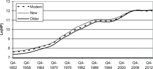
Figure 1 shows the smoothed or trend part of the house price time series. The data, in logarithm form, highlight a similar pattern of growth that would correspond with common trends in a cointegrated system, which authors investigating a ripple effect in regional prices had found, such as Alexander and Barrow (1994). The trend in Older housing is more steep, switching from the least to the most expensive of the three vintages. Modern house price grew at an annual rate of 7.779%, slightly lower than New at 7.795% but slower than Older at 8.421%.

Figure 1. Smoothed house prices.

With the trend element removed, the standard deviations of the cyclical components in the time domain are estimated. Modern (.0512) and Older (.0521) exhibit greater volatility than New (.0480). In other words, there is greater price variation around the trend in second-hand than New.

6. Results

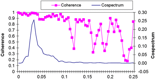
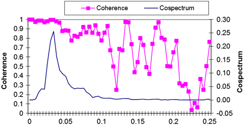
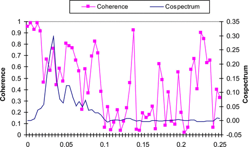
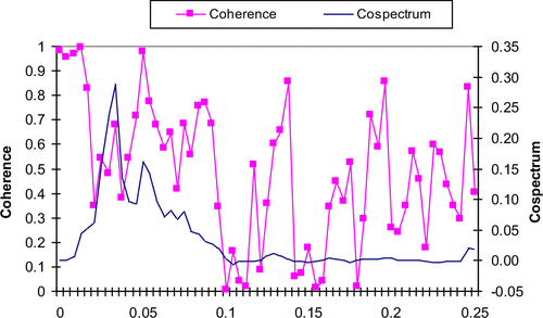
The spectra between New and Modern housing are plotted in Figure 2, and New and Older in Figure 3. The cospectra show a single peak at a 7½-year cycle. At this and across the lower frequencies, the coherence values are 0.9 and above, suggesting a close association consistent with those among substitutes. The single spike with a high coherence value indicates price comovement of New and Modern at a common dominant cycle.

Figure 2. New-Modern coherence and cospectrum against fractions of π radians.

Figure 3. New–Older coherence and cospectrum.

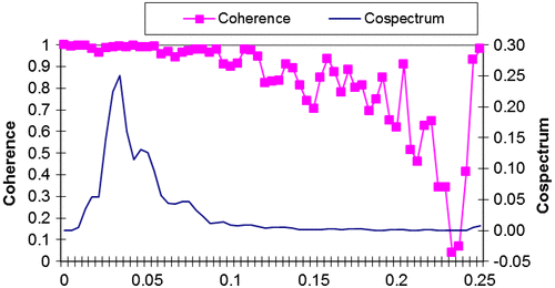
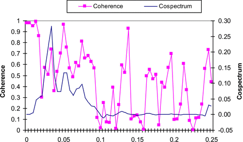
Comparing the coherence among Modern and Old in Figure 4 with those of New and Modern, and New and Older suggests the values are all high around 7½ year cycles, but the second-hand pair remain closely associated at the 5.45-year cycle. The cospectra all show a peak at a 7½-year cycle, but second-hand housing display a peak at 5.45 the cycle. It is inferred that second-hand housing exhibits a greater level of covariation than between either with New.

Figure 4. Modern–Older coherence and cospectrum.

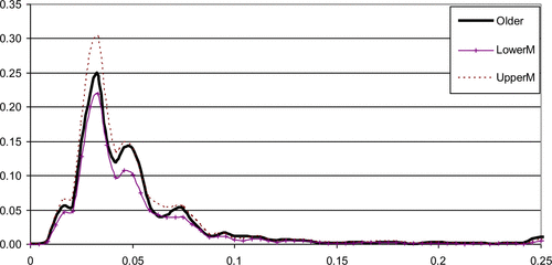
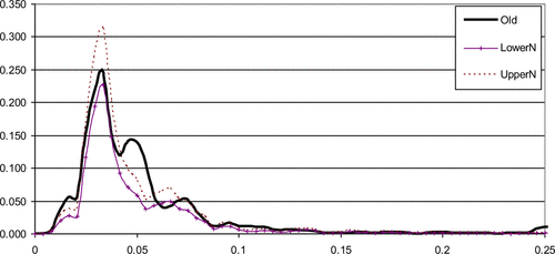
A closer bond between second-hand markets should be reflected in their power spectra. The Older power spectrum values are displayed in Figure 5 with the 95% confidence intervals for Modern prices. As with the cospectrum, the variation of interest is found at the lower frequencies. As all key values of one fall within the confidence intervals of the other, it is concluded that the volatility of the Older and Modern housing across the spectrum are indistinguishable and that the two series have common cycles.

Figure 5. Older power spectrum.

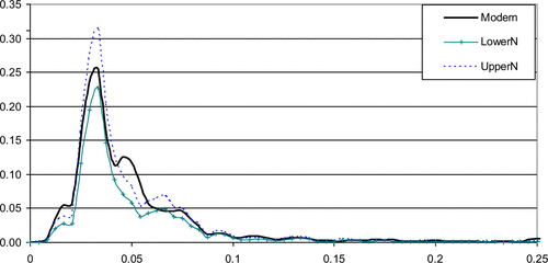
Next, the New and Modern price volatilities are compared. Using the confidence intervals of New housing, the Modern and Older power spectra values in Figures 6 and 7 are above upper bounds at 15 and the 5.45 year cycles, and below at the 3¾.

Figure 6. Modern power spectrum.

Figure 7. Older power spectrum.

It appears that there is a considerable proportion of power and covariation among the three vintages between 15 and 2½-year cycles, particularly around 7½ years, suggesting that Cook and Holly’s common cycles are somewhere between these two. With the peaks of the spectra at 7½ years featuring so prominently and so little power elsewhere, one can assert that there are common cycles among the three vintages. Dicks (1989) postulates a system where there is a seven-year lag between moves, which give broadly the “right” number of RBs in the market. Levy and Dezhbakhsh (2003) define business cycles as being in the range 3–8 years. They show UK GDP as having a single peak at around 6–8 years, which put that housing cycle revealed towards the longer end.

Cook and Holly’s (2000) asynchronised common cycles might be related to slight phase differences. At the 7½-year cycle, the phase values between Modern and Older suggest the latter follows the former by around three weeks with New delayed by a further week. Modern house prices may be used as a marker for the valuation of Older properties. By contrast, at the 5.45 cycle, Modern leads Older by six weeks, and New precedes Modern by half that. New prices might be a leading indicator of general market supply conditions. The 3¾-year cycle again highlights a 2- to 3-week (17 days) delay between Modern and Older but Modern leads New by eight weeks. The Older–Modern delay is consistent with the 7½-year but New switches from follower to leader. These figures do suggest a notable asynchrony, but not at a level that Cook and Holly could discern. Indeed, a switching of phase may leave inferences in time domain analysis somewhat blurry.

To summarise, the Modern and Older have indistinguishable power spectra, signifying that they are substitutes with common cycles. In a ripple sense, Modern house prices lead and signal changes will affect Older properties around 3–6 weeks later. Nevertheless, as posited, Modern and Older housing vintages are found to be distinct from New. They follow New at the 5.45-year cycle, where the latter has lower volatility than the former two, which is the most distinguishing feature.

7. Construction expenditure

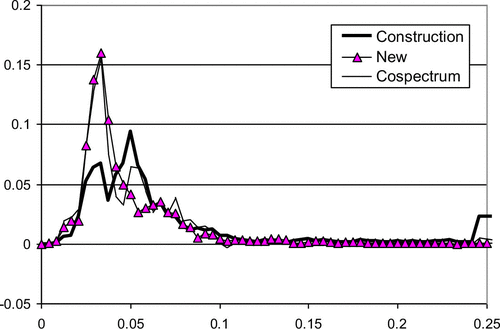
The normalised power and cospectrum for New house prices and construction are displayed in Figure 8. The cycles that are prominent in construction are 7½, 5 and the 3¾ years. However, the concentration of volatility in prices is greater than in construction. These results resonate with Barras and Ferguson’s finding of a major cycle of 6½ years for New orders for private housing construction in the UK data (supply cycle), which is distinguished from a second, shorter 3¾-year cycle (demand cycle).

Figure 8. Expenditure-New power spectra and cospectrum.

The cospectrum highlights four peaks (7½, 5, 3¾ and 3.33 year cycles). The phase values point to a lead of construction expenditure over prices. If these were building “starts”, that would confound the expected causation. As with price analysis, Modern and New switch places. At the 7½-year cycle, expenditure leads Modern prices by 6.1 months, Older by 7.3 months and New by 7 months. At the 5-year cycle, New prices follow expenditure at a delay of 9 months, with Modern reacting two weeks later and Older a further five weeks after that. These delays are too long for a price response. Brinkley (unknown) suggests eight months is the average time it takes to build a detached house in the UK. These delays could be capturing the time it takes to construct a New dwelling before it affects prices.

When considering the cospectra displayed in Figures 9Figure 10.–11, all exhibit at least two major cycles, including New house prices. Coherence is relatively high for all. Activity in construction should affect pricing volatility at the five and 7½-year cycle. Where it has a lower volatility density, construction will have a smaller moderating effect on price.

Figure 9. Construction with New prices.

Figure 10. Construction with Modern prices.

Figure 11. Construction with Older prices.

DiPasquale and Wheaton’s myopic model predicts cycles of building and pricing such that construction sector would build sufficient houses to drive prices down. A positive relationship at both cycles could be explained by a weak output response to price, which has been a feature of UK housing (Meen, 2000, 2005). This lack of an inverse relationship suggests that excess supply of New dwellings is not a common feature of the UK’s housing market. The Barker (2003) report highlights vested interests in maintaining low output among local authorities, homeowners and builders. The planning process is restrictive and insensitive to price signals. The industry itself to manage price volatility acts to restricts the supply of New builds but is also short of skilled workers, which also constrains construction.

Two points could be made here about the weak supply response. First, an alternative explanation for a collapse in house prices could rely on other factors, most likely among them is unaffordability of mortgage payments. Perhaps, the so-called Minsky point is passed, where mortgage interest payments cannot be met. Second, the claim that release of New builds is orchestrated to reduce price volatility could be reflected in the single power spectrum spike in New housing mentioned above.

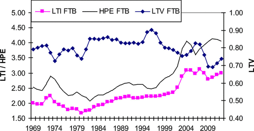
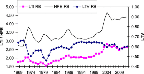
Minsky’s super-cycle relates to trends in financing. In Figures 12(a) and 12(b), the house price-earnings ratio (HPE), a standard measure of housing affordability, is displayed. It can be broken down into two elements. The LTI is a multiple of the loan relative to average income of the borrower. The LTV is the same loan relative to the house price upon which the loan is secured, providing some idea of the down payment or equity a buyer needs to purchases a property. The HPE indicates the least affordability when the LTI is at a peak and the LTV is in a trough.

Figure 12a. Loan to income and value ratios FTB.

Figure 12b. Loan to income and value ratios RB.

One would expect that LTV, which is much higher for the FTB than that of the RB, is the more important constraint in the case of the former. With growing embedded equity, as prices rise, the LTV becomes much less of a constraint for the RB. For them, it is the permitted income multiple that limits their purchase. For the RB in Figure 12(b), the HPE peaks are in 1973, 1979, 1989 and 2004. As highlighted by the HPE, the years of least affordability for the FTB are revealed as 1973, 1991, 2003 and 2010. There is some correspondence with RBs.

It is interesting to observe an upward trend in LTI from 1980 to 2004. Although it does not correspond with a super-cycle, it does fit with a Minsky thesis that financial constraints were relaxed over a long period, and hit a maximum at a price turning point.

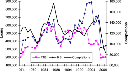
Figure 13 displays number of buyers and the number of dwelling completions. The number of completed properties peaks in 1975, 1988 and 2007. The number of FTBs in the market is at local maxima in 1977/1999, 1986/1988, 1994, 1999 and 2006. For RB, the corresponding years are 1979, 1988, 1993 and 2004, which coincide less regularly than one might expect.

Figure 13. Completions and numbers of buyers with mortgages in the market.

One can see peaks in the numbers of loans to RBs coinciding with HPE maxima. In other word, participation is at a high when houses are “least affordable”. The years 1973, 1989 and 2004 precede a housing crash. The FTB seems more prudent. The peaks of the LTV are in 1978, 1986, 1996 and 2006, suggesting that FTBs participate in the market when the finances are favourable and are priced out before a price collapse. This is consistent with price rises favouring the owner and speculative market activity.

It was posited that there would be a change in the constitution of the market with rising price. A surge in activity began in 1995. The number of FTBs hit a peak in 1999, five years before that of the RB, when houses were there most expensive for 15 years. The FTB’s average down payment had risen from 27% of average income to 53%. Both RBs and FTBs saw a peak in their HPE ratio in 2004, but the numbers of FTBs affected would be relatively modest: the number of FTBs was 38% below the number in 1988, whereas in 2004, the number of RB was up by 32%.

8. Discussion

Chen et al. (2004) argue that monetary cycles tend to correspond with increased demand in the housing market. Meen (2000) concludes that monetary policy in the UK can incite price cycles. Pakko (2000) utilises the cospectrum to show both positive and negative relationships among output (GNP) and prices (CPI) in the USA over 120 years. He posits that output should have a negative effect on prices, but a positive money shock would increase output and prices, at least in the short run. He concludes that a dual shock model offers superior simulations compared with a single shock model.

The peaks in the RB’s HPE are separated by a 15-year interval. There is possibly of a 15-year divide between peaks in LTI ratio, which points to finance being a driver of house prices, consistent with a Minsky super-cycle and its underlying causes. This peak in house price activity could reflect the RB with capital constraints, taking advantage of greater equity, revisiting the market. As the market picks up, more rejoin, adding volatility in a Stein sense. With innovative products, financial institutions fuel this activity by accommodating the increasing absolute gap between income and house price, which again is consistent with Minsky. This implies that the number of RBs, sellers and funding for the exchange of houses are pro-cyclical. The maximum number of mortgage-seeking RBs in the market corresponds with the peak in prices.

The spectral results here appear consistent with prices and quantities following a 7½ and 5 cycle. Construction expenditure and prices are revealed to covary strongly at, at least, two cycles. A five and a 7½-year cycle would interfere or reinforce each other every 15 years. Thus, a possible inference from the construction-price cycles is the notion of a super-cycle. There is no negative or downward pressure due to supply, possibly due to a modest construction sector and the enormity of the response that this sector would have to provide (Meen, 2005), or Pakko’s positive monetary shock.

Builders increase expenditure in constructing New dwellings that come on stream eight months later. Once they are on the market, one might suggest the pricing could be seen as supply-led (five year cycle) or demand driven (7½-year cycle). This paper here proposes an alternative view of the dual spike: there is a shorter and more muted FTB-NEW housing-focused cycle and a longer more pronounced RB-second-hand cycle. FTBs mollify house price volatility and New builds extract embedded equity from the market. This postulate can explain the weaker second spike with house price series.

Stein and Ortalo-Magne and Rady’s contributions highlight the role of the down payment combined with adjustable lending criteria. Minsky’s super-cycle explains why lending can get out of hand. However, the fulcrum around which the volatility swings is the growth of embedded equity. If this were extracted, subject to a sizeable windfall sales tax, the RB would be less likely to rejoin the housing market as prices begin to accelerate, house prices would be much less volatile as a result.

9. Conclusion

This paper set out to consider common cycles in housing vintages in the UK using spectral analysis. Spectral analysis can reveal hidden periodicies in the frequency domain that are not evident in the time domain.

Over the sixty years considered there is evidence of a 7½-year cycle common to New, Modern and Older house prices in the UK. This is also reflected in construction expenditure. This is consistent with Alexander and Barrow (1994) and Rosenthal (1986) with UK house prices and Levy and Dezhbakhsh (2003) and GDP volatility across the spectrum. There is a second cycle of around five years found in the four series.

The work makes two contributions to Hui’s (2011) house price dynamic classifications. There is a house price ripple in cycles from Modern to Older dwellings. As such, we can add a fourth strand in ripple effect literature. Also, as New has lower volatility, this would correspond with Hui’s (2011) third strand.

There is a series of contributions to the literature. Revealing a small number of key cycles leads to a consideration of the underlying driver of each. Others have found more than one spike, ascribing them to supply and demand factors. Distinguishing between FTBs and RBs, and between New and second-hand housing are central themes of this analysis. It is also proposed that that the FTB is more closely linked to the shorter cycle. Arguing that the presence of both New housing and FTB has the effect of lowering volatility, this could explain why one of the three price series is distinct. Further investigation of this dual cycle phenomenon could confirm whether the proposition that they reflect two groups of buyers is supported.

A 5 and a 7½-year cycle would reinforce each other every 15 years. This is reflected in prices and construction. Moreover, symptoms of a Minsky super-cycle of that order are revealed in housing finance.

Some policy implications of the analysis outlined here concern the regulator and a policy initiative. Minksy’s analysis on the reaction to a crisis suggests that tighter regulation will follow. In September 2014, the Bank of England’s Financial Policy Committee (2014) was considering setting limits on mortgage lending ratios. If left to the market, any commitment to self-regulation will leave us back to a crisis within a decade.

The introduction of the Help-to-Buy 1-equity scheme in April 2013 was a reaction to a thin housing market and low construction levels in the UK. Restricted to FTBs and targeting the construction of New homes, the scheme proffers a LTV of 95% at the outset whilst extracting a fifth of the growth in housing equity. It has two elements that mollify market volatility. It reduces the required down-payment at the outset, extracts embedded equity at the end of the loan, and guides buyers away from second-hand houses. By contrast, Help-to-Buy 2, introduced in October 2013, is a mortgage guarantee scheme that also raises the LTV available to 95%. It is open to all buyers purchasing housing of any vintage. This scheme should increase volatility, inflating prices beyond that pocket of the FTB. If the government were prepared to extract some equity through a capital gains tax, the scheme would have some merit. With an election in 2015, it is perhaps is good politics to boost property prices and, hence, capital gains, rather than good social policy.

Additional information

Funding

Funding. The authors received no direct funding for this research.

Notes on contributors

David Gray

David Gray is academic leader of the Division of Accounting, Finance and Economics at University of Lincoln. His interests include: House Price Dynamics, Exchange rates and Contagion, and Regional Labour Markets. This contribution can be seen as part of a theme concerning ripples in house prices.

Appendix A

The theoretical spectrum divides up a time series into a set of components that are orthogonal. It reveals the relative power at each frequency corresponding to the variance at each periodicity, so that sharp peaks denote a high concentration. The autocovariance ${\mathit{\gamma }}_{XX}(k)=E\left[(X_{t+k}-\mathit{\mu })(X_t-\mathit{\mu })\right]$ in the time domain is represented as $s_{XX}(\mathit{\omega })=\frac{1}{2\mathit{\pi }}\sum _{k=-\infty }^{\infty }{\mathit{\gamma }}_{XX}(k)e^{-ik\mathit{\omega }}$ in the frequency domain. As the periodogram does not provide a consistent estimate of the theoretical spectrum, smoothing is required. There is a trade-off between stability and fidelity. The power spectrum is given by ${\widehat{s}}_{XX}(\mathit{\omega })=\frac{1}{2\mathit{\pi }}\sum _{k=-M}^{M}w\left(k\right){\widehat{\mathit{\gamma }}}_{XX}\left(k\right)e^{-i\mathit{\omega }k}$. The 95% confidence band for the spectrum with v = equivalent degrees of freedom is given by ${\widehat{s}}_{XX}(\mathit{\omega }){\left(1\pm 1.96\sqrt{2/v}\right)}^{-1}$. The corresponding expression of the cross-spectrum, ${\widehat{s}}_{XY}(\mathit{\omega })=\frac{1}{2\mathit{\pi }}\sum _{k=-M}^{M}w\left(k\right){\widehat{\mathit{\gamma }}}_{XY}\left(k\right)e^{-i\mathit{\omega }k}$, can be broken down into the real and imaginary parts, $s_{XY}(\mathit{\omega })=c_{XY}(\mathit{\omega })-i{q}_{XY}(\mathit{\omega })$, where the cospectrum is defined as $c_{XY}(\mathit{\omega })=\frac{1}{2\mathit{\pi }}\sum _{k=-\infty }^{\infty }{\mathit{\gamma }}_{XY}(k)cos(\mathit{\omega }k)$. The cospectrum between X and Y at frequency ω_j represents the covariance between X and Y at frequency ω_j (Hamilton, 1994). Coherence is the frequency domain equivalent of squared correlation. If the coherence is large, it indicates the degree to which X and Y are jointly influenced. The estimated squared coherence is given by ${{\widehat{C}}_{XY}}^2(\mathit{\omega })=\frac{{\left|{\widehat{s}}_{XY}(\mathit{\omega })\right|}^2}{{\widehat{s}}_X(\mathit{\omega }){\widehat{s}}_Y(\mathit{\omega })}$ (Jenkins & Watts, 1968). The Phase value gives a notion of leading (if positive) of the first series X over the second Y. The estimated phase angle ${\widehat{P}}_{XY}(\mathit{\omega })={tan}^{-1}\frac{-{\widehat{q}}_{XY}(\mathit{\omega })}{{\widehat{c}}_{XY}(\mathit{\omega })}$. For a given P_XY(ω_j), the time shift is tau τ = phase angle/angular frequency P_XY(ω_j)/ω_j which can be written as P_XY(ω_j)/2πf_j (Harvey, 1993).

T = 240 with smoothing across three points with a Parzen lag window, where v is the number of degrees of freedom (=298).

References

- Alexander, C., & Barrow, M. (1994). Seasonality and cointegration of regional house prices in the UK. Urban Studies, 31, 1667–1689.https://doi.org/10.1080/00420989420081571
- Barker, K. (2003). Review of housing supply: Interim report—Analysis. London: HMSO.
- Barras, R., & Ferguson, D. (1985). A spectral analysis of building cycles in Britain. Environment and Planning A, 17, 1369–1391.https://doi.org/10.1068/a171369
- Benito, A. (2006, March). How does the down-payment constraint affect the UK housing market? ( Bank of England Working Paper 294). London: Bank of England.
- Bover, O., Muellbauer, J., & Murphy, A. (1989). Housing. Wages and UK labour markets. Oxford Bulletin of Economics and Statistics, 51, 367–382.
- Brinkley, M. (unknown). How fast can you build a House? Homebuilding and renovation. Retrieved September 26, 2014, from www.homebuilding.co.uk
- Canova, F. (1999). Does detrending matter for the determination of the reference cycle and the selection of turning point? The Economic Journal, 109, 125–150.
- Chen, M.-C., Kawaguchi, Y., & Patel, K. (2004). An analysis of the trends and cyclical behaviours of house prices in the Asian markets. Journal of Property Investment & Finance, 22, 55–75.
- Cogley, T., & Nason, J. (1995). Effects of the Hodrick–Prescott filter on trend and difference stationary time series implications for business cycle research. Journal of Economic Dynamics and Control, 19, 253–278.https://doi.org/10.1016/0165-1889(93)00781-X
- Cook, S., & Holly, S. (2000). Statistical properties of UK house prices: An analysis of disaggregated vintages. Urban Studies, 37, 2045–2051.https://doi.org/10.1080/713707230
- Coulson, N., & Mcmillen, D. (2007). The dynamics of intraurban quantile house price indexes. Urban Studies, 44, 1517–1537.https://doi.org/10.1080/00420980701373446
- Dicks, M. (1989, February). The housing market. Bank of England Quarterly Bulletin, pp. 66–75.
- DiPasquale, D., & Wheaton, W. (1996). Urban economics and real estate markets. Englewood Cliffs, NJ: Prentice Hall.
- Dusansky, R., & Wilson, P. W. (1993). The demand for housing: Theoretical considerations. Journal of Economic Theory, 61, 120–138.https://doi.org/10.1006/jeth.1993.1061
- Financial Policy Committee. (2014, October 2). Statement. Bank of England. Retrieved November 13, 2014, from http://www.bankofengland.co.uk/financialstability/Documents/fpc/statement021014.pdf
- Gray, D. (2012). District house price movements in England and Wales 1997–2007: An exploratory spatial data analysis approach. Urban Studies, 49, 1411–1434.https://doi.org/10.1177/0042098011417020
- Hamilton, J. (1994). Time series analysis. Princeton, NJ: Princeton University Press.
- Harvey, A. (1993). Time series models (2nd ed.). Hemel Hempstead: Harvester Wheatsheaf.
- Ho, L., Ma, Y., & Haurin, D. (2008). House price changes across quality tiers. Journal of Real Estate Finance & Economics, 37, 299–316.
- Hughes-Hallett, A., & Richter, C. (2004). Spectral analysis as a tool for financial policy: An analysis of the short-end of the British term structure. Computational Economics, 23, 271–288.https://doi.org/10.1023/B:CSEM.0000022836.40541.9f
- Hui, H.-C. (2011). Cycles in landed and non‐landed housing sub‐markets in Malaysia. International Journal of Housing Markets and Analysis, 4, 144–154.https://doi.org/10.1108/17538271111137921
- Jenkins, G., & Watts, D. (1968). Spectral analysis and its applications. London: Holden-Day.
- King, R., & Rebelo, S. (1993). Low frequency filtering and real business cycles. Journal of Economic Dynamics and Control, 17, 207–231.https://doi.org/10.1016/S0165-1889(06)80010-2
- Levy, D., & Dezhbakhsh, H. (2003). International evidence on output fluctuation and shock persistence. Journal of Monetary Economics, 50, 1499–1530.https://doi.org/10.1016/j.jmoneco.2003.08.005
- Liow, K. H. (2007). Cycles and common cycles in real estate markets. International Journal of Managerial Finance, 3, 287–305.https://doi.org/10.1108/17439130710756925
- Maclennan, D., Muellbauer, J., & Stephens, M. (1998). Asymmetries in housing and financial market institutions and EMU. Oxford Review of Economic Policy, 14, 54–80.https://doi.org/10.1093/oxrep/14.3.54
- Mayer, C. (1993, May–June). Taxes, income distribution, and the real estate cycle: Why all houses do not appreciate at the same rate. New England Economic Review, pp. 39–50.
- Meen, G. (1996). Spatial aggregation, spatial dependence and predictability in the UK housing market. Housing Studies, 11, 345–372.
- Meen, G. (1999). Regional house prices and the ripple effect: A new interpretation. Housing Studies, 14, 733–753.https://doi.org/10.1080/02673039982524
- Meen, G. (2000). Housing cycles and efficiency. Scottish Journal of Political Economy, 47, 114–140.https://doi.org/10.1111/sjpe.2000.47.issue-2
- Meen, G. (2005). On the economics of the barker review of housing supply. Housing Studies, 20, 949–971.https://doi.org/10.1080/02673030500291082
- Office for National Statistics. (2014). House price index (HPI). Newport: Author.
- Ortalo-Magne, F., & Rady, S. (2006). Housing market dynamics: On the contribution of income shocks and credit constraints. Review of Economic Studies, 73, 459–485.https://doi.org/10.1111/roes.2006.73.issue-2
- Pakko, M. (2000). The cyclical relationship between output and prices: An analysis in the frequency domain. Journal of Money Credit and Banking, 32, 382–399.https://doi.org/10.2307/2601171
- Palley, T. (2010). The limits of Minsky’s financial instability hypothesis as an explanation of the crisis. Monthly Review, 61, 28–43.https://doi.org/10.14452/MR-061-11-2010-04
- Palley, T. (2011). A theory of Minsky super-cycles and financial crises. Contributions to Political Economy, 30, 31–46.https://doi.org/10.1093/cpe/bzr004
- Pyhrr, S., Roulac, S., & Born, W. (1999). Real estate cycles and their strategic implications for investors and portfolio managers in the global economy. The Journal of Real Estate Research, 18, 7–68.
- Renaud, B., Zhang, M., & Koeberle, S. (1998, May 20). How the Thai real estate boom undid financial institutions—What can be done now? In Conference on Thailand’s dynamic economic recovery and competitiveness. Bangkok. Retrieved from http://citeseerx.ist.psu.edu/viewdoc/download;jsessionid=E314B03D2C9B39A31AAC1582D7EFFD40?doi=10.1.1.196.1373&rep=rep1&type=pdf
- Rosenthal, L. (1986). Regional house price interactions in the UK, 1975–81: A cross-spectral analysis. Applied Economics, 18, 1011–1023.https://doi.org/10.1080/00036848600000057
- Smith, L., & Ho, M. (1996). The relative price differential between higher and lower priced homes. Journal of Housing Economics, 5, 1–17.https://doi.org/10.1006/jhec.1996.0001
- Stein, J. (1995). Prices and trading volume in the housing market: A model with down-payment effects. The Quarterly Journal of Economics, 110, 379–406.https://doi.org/10.2307/2118444
- Wilson, P., & Okunev, J. (1999). Spectral analysis of real estate and financial assets markets. Journal of Property Investment and Finance, 17, 61–74.https://doi.org/10.1108/14635789910252909