A classroom game to teach the principles of money and banking

Abstract

This paper describes how to implement and run a game for teaching the principles of money and banking to an undergraduate economics class. The game primarily deals with the market for loanable funds, but numerous extensions are provided to cover topics such as monetary policy, the tools of the Federal Reserve, shifts in the equilibrium of the market for loanable funds, and the quantity theory of money. The experiment can be used in principles, intermediate macroeconomics, or money and banking courses. The experiment takes approximately 45 minutes to run, depending on class size, and requires no computers.

Keywords:

• money and banking
• market for loanable funds
• teaching
• economics education
• games
• experiments
• economic tools for teaching

JEL classifications:

• A22
• C9
• E42

Public Interest Statement

This paper describes how to implement and run a game for teaching the principles of money and banking to an audience interested in economics. The game requires no real background in economics to play and takes only about 45 minutes, depending on audience size. The game can be a great means of teaching economics tools or the game can be used to stimulate interest in economics to a nontraditional audience. The game can be used to highlight the role of a central bank and the importance of the market for loanable funds.

1. Introduction

This paper introduces a game that educates students by having them participate as rational economic actors in a market for loanable funds. The game is designed to teach students to apply basic market principles to the market for loanable funds.

While a large literature exists for microeconomic proactive pedagogy (Crowley & Hoffer, 2015; Hoffer, 2014; Holder, Hoffer, Al-Bahrani, & Lindah, 2015; Rousu et al., 2015; Smith, Williams, Bratton, & Vannoni, 1982), macroeconomic topics have seen far less attention in the literature. Several money-related macroeconomic games exist, but their focus is different than the micro-funded incentive-based market for loanable funds used in this study.

Hester (1991) uses a computerized simulation to examine bank portfolio management; Cameron (1997) and Laury and Holt’s (2000) describe games to examine money creation; Hazlett’s (2003) game is a federal funds market experiment; Balkenborg, Kaplan, and Miller (2011) focuses on bank runs; and Kassis, Hazlett, and Battisti (2012) use a double oral auction credit markets to illustrate the role of banks as financial intermediaries, specifically focusing on the way in which risk affects market interest rates in the presence of asymmetric information.

The game I present in this paper is designed to utilize micro-level incentives, often covered in microeconomics, to create a market for loanable funds that parallels the market for goods and services that is often the focus of most microeconomics courses and some macroeconomics principles courses. The game is based on Smith et al.’s (1982) pit auction experiment. In the simplest, quickest form, the game covers the basic principles of the market for loanable funds. This paper also presents several extensions to the game that can be used to teach higher level macroeconomic topics, market equilibrium processes, shifts in equilibrium, and the role and effects of the Federal Reserve. Simple modifications can also make the game suitable for small class sizes or for large lecture halls.

2. The game

2.1. Base version

The goal of this game is to make as much profit as possible. Firms earn profit by acquiring loanable funds from banks to complete projects. The quantity of funds necessary to fund various projects and the corresponding profit each project yields the firm are listed on each firm’s handout. Conversely, banks earn profit by lending funds to firms and charging interest for those funds. In order to complete a transaction, the firm and the bank must agree on the total amount of funds to be transferred and the interest rate. Interest on funds will be paid only one time, at the end of the round; and no principle is to be repaid. The banks’ profit is solely a function of interest collection (Appendix A).

Tables 1 and 2 describe the game setup. Banks begins with a fixed quantity of funds. Firms need loans in order to fund projects, which in turn create profit for the firm.

Table 1. The supply of loanable funds

Bank 1 funds available: $18,000

Bank 2 funds available: $14,000

Bank 3 funds available: $11,000

Bank 4 funds available: $7,000

Table 2. The demand for loanable funds

Firm	Project	Funds received ($)	Profit generated ($)	Profit (%)
Firm 1	1	100,000	45,000	45
	2	6,000	600	10
	3	5,000	400	8
	4	1,000	50	5
Firm 2	1	50,000	5,000	10
	2	10,000	700	7
	3	5,000	250	5
	4	3,000	90	3
Firm 3	1	15,000	1,500	10
	2	7,000	490	7
	3	4,000	200	5
	4	1,000	10	1
Firm 4	1	5,000	2,000	43
	2	4,000	1,200	30
	3	3,000	600	20
	4	2,000	100	5

Any projects not funded by firms and any funds not loaned by banks earned zero profit (there is zero benefit and zero explicit penalty for holding reserves or not funding a project). The winners of the game will be the firm and the bank which are able to create the greatest profit.

An example transaction is illustrated in Table 3. Firm X receives $5,000 from bank Y at 5% interest ($250). With that $5,000, firm X funds Project 2, generating an additional $500 in revenue. Subtracting the $250 in interest payments, firm X generates a $250 profit. Bank Y generates $250 in interest profit.

Table 3. Example transaction

Firm X
Period one
Project	Funds required ($)	Revenue generated ($)	Revenue (%)
1	10,000	1,500	15
2	5,000	500	10
3	2,500	125	5
4	1,000	10	1
Transactions log
Funds received ($)	Interest paid (%)	Net profit (%)	Profit generated ($)
5,000	5	5 (10−5%)	250

Bank YRound 1
Funds available ($)	Loan given ($)	Interest collected (%)	Profit ($)	Loans taken	Interest paid	Total profit ($)
20,000	5,000	5	250	–	–	250
15,000

Each round concludes upon reaching a predetermined time constraint or when market activity ceases. To publicize market activity and to save transaction data for future use, the interest rate for each transaction is listed on the board immediately following the agreement and the data are stored in the Economic Science Institute’s free Double Auction program (Jaworski, Kirchner, & Wilson, 2008).

2.2. The Federal Reserve discount window

Following the conclusion of Round 1, the Federal Reserve discount window (Fed) is introduced in Round 2. Round 2 is exactly identical to Round 1, with the following exception. The Fed has an infinite sum of money and will lend to any bank at a fixed interest rate of 1%. The role of the Fed can be played by the instructor or any additional player that is not already participating in the game.

Introducing the central bank provides instructors with an opportunity to discuss the role of a central bank and Federal Reserve Bank policy. Instructors may find this particularly relevant in light of Federal Reserve Bank actions following the Great Recession. From December 2008 until the writing of this manuscript, The Federal Funds rate has been 0.25% or less. The primary goal of such a low interest rate was economic stimulation, something that can be easily illustrated using the Fisher’s Quantity Theory of Money and short-run fiscal policy. In the simplified classroom experiment, assuming away price (P) and velocity (V) from the Fisher equation MV = PY, yields M = Y. Clearly the extra money made available to firms allowed a substantial increase in production. Professors may also find this a great time to review inflation.

2.3. Pedagogical note following the game’s conclusion

Only after the game is finished do I present the actual textbook image of the market for loanable funds. By this time, the students’ have already crafted what the market will look like. Ask the students, “Firms, what kind of interest rate did you want to negotiate?” The answer is the lowest possible interest rate. Therefore, at high interest rates, fewer firms were demanding loanable funds; and, at lower interest rates, more firms were demanding loanable funds. Students playing the role of firms could have easily drawn a downward sloping of loanable funds curve. Students playing the role of bankers could just as easily identify the upward sloping supply of loanable funds curve.

Following the discussion of the theoretical “textbook” market for loanable funds, I bring back the data collected from the game in which the students just participated. Using the interest rates recorded during each round, I present and discuss the gains from trade in the market for loanable funds. With each transaction, students can get a visual representation of borrower and lender surplus, analogous to consumer and producer surplus, for each transaction, a topic not thoroughly discussed in most principles textbooks, by substituting the interest rate for price on the vertical axis.

3. Results from a classroom case study

I recorded the results from a two-round game played in a 16-student principles of macroeconomics class. Round 1 consisted of just the base version and Round 2 added the Federal Reserve discount window. The transactions from Round 1 are presented, in order, in Table 4 and the market interest rate negotiated are illustrated in Figure 1. While there were no direct costs of holding excess reserves or failing to fund a project, the opportunity costs of such activities were obvious. Therefore, time spent negotiating carried a pricy opportunity cost, potentially preventing a student from transacting with a different buyer/lender within the fixed time period for Round 1.

Table 4. Classroom results from Round 1

Bank	Firm	Amount	Interest rate	Bank profit	Firm profit
1	2	10,000	7.5	750	−50
2	1	8,000	8	640	160
2	2	3,000	4.5	135	−85
4	3	7,000	7	490	0
3	1	5,000	8	400	0
1	3	1,000	10	100	−90
1	4	5,000	8	400	1600
1	1	1,000	6.5	65	−15
2	4	2,000	4	80	200
3	4	4,000	8	320	880
3	2	2,000	10	200	N/A^a
1	4	1,000	2	20	−20

^a This transaction was combined with a $3,000 loan to fund a $5,000 project. Total losses on this project are noted with the $3,000 project in row three.

Figure 1. Round 1 transaction interest rates.

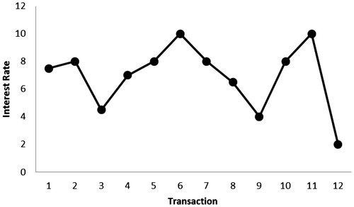
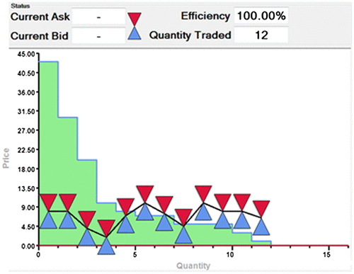
The results from Round 1 illustrate a divide among students who understood how to make a profit in the game and those who did not. Of the 12 transactions made in Round 1, only four transactions were profitable for firms—an admittedly sad result when trying to illustrate mutual gains from trade. Borrow and lender gains from trade are displayed in Figure 2. With zero lending costs for banks, every transaction was profitable for banks. However, after taking a few minutes to calculate profits, congratulate winners of Round 1, and hand out bonus points (tangible “bonus buck” certificates), students who struggled in Round 1 were able to identify how it is that banks and firms make profits by exchanging money.

Figure 2. Borrower/lender gains from trade.

In Round 2, every transaction was mutually profitable, illustrated in Table 5 and Figure 3.¹ Clearly, students learned that a well-negotiated interest rate make it possible for both lenders and firms to profit. By including the Fed, banks were now able to cheaply fill their coffers and eliminate the shortage of funds. It was now possible for firms to fund every project on their production sheet.

Table 5. Classroom results from Round 2 (with Fed)

Bank	Firm	Fed	Amount	Interest rate	Bank profit	Firm profit
1		x	32,000	1	−320	–
4		x	100,000	1	−1,000	–
1	2		50,000	9	4,500	500
4	1		100,000	4	4,000	41,000
2	3		4,000	6	240	40
1		x	5,000	1	−50	–
1	4		5,000	2	100	1,900
3	1		8,000	9.5	760	40
2	2		5,000	4.5	225	25
1		x	5,000	1	−50	–
1	1		5,000	6	300	100
4		x	4,000	1	40	–
4	4		4,000	5	200	1,000
2	1		1,000	3	30	20
1		x	3,000	1	−30	–
1	2		3,000	2	60	30
2	4		3,000	4	120	480
3		x	7,000	1	−70	–
3	2		10,000	5	500	200
1		x	2,000	1	−20	–
1	4		2,000	3	60	40
4	3		7,000	2	140	350

Figure 3. Round 2 borrower/lender gains from trade.

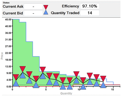
This is the first of many changes from Round 1 to Round 2 that can be referenced later with saved data from the experiment to illustrate learning objectives. The introduction of the Fed—an increase in loanable funds—increased the number and quantity of loanable funds transactions. The interest rate also was much lower in Round 2. Both of these market changes are great to reference when discussing shifts in equilibrium.

4. Extensions

4.1. Finding an equilibrium

Initial parameter and instructional changes:

Forced ordering: Once a firm funds a project, it cannot fund a higher order project. For example, once firm X funds project 3, firm X may no longer fund projects 1 or 2 if they have not already been funded. This involves earmarking of funds to projects, i.e. a firm cannot simply collect funds and decide what projects to fund post hoc. This “pushes” the market, with respect to interest rates, to an equilibrium.

4.2. Shifts in equilibrium

Round 1: See Extension 4.1: Finding an Equilibrium.

Round 2: Modify any of the shift variables of the firms (e.g. a monotonic increase in the profit percentage earned on each project by 5% shifts the equilibrium interest rate upwards) or change any of the shift variables of the banks (e.g. Extension 1 provides banks with additional loanable funds, therefore shifting the equilibrium interest rate downwards).

4.3. Nonzero bank costs

4.3.1. Fixed costs

Opportunity costs of lending and/or a processing fee: For banks, we can assume that any funds the bank has can “safely” be invested in treasury bills or bonds at a low interest rate. This would be an excellent place to use the current US long-term bond rate as a real-world example. The result of this should simply be a shift in the supply of loanable funds curve.

4.3.2. Variable costs and an upward sloping supply of loanable funds

Costs of lending: By introducing costs that either vary by firm (creating a supply for loanable funds that is flat for each individual firm, then “jumps” up and is flat for the next firm), creating costs that are inversely related to the interest rate (i.e. cost = 0.10*i), or instituting some combination of the two, can create an upward sloping supply for loanable funds curve.

4.4. Larger audiences

This game was initially designed for 16 participants (8 pairs or students). The first solution to expanding this game to larger audiences is to simply add more firms and banks. If collection and reporting of the data becomes problematic, a few solutions are available. Instead of pairs of students, students can be placed in larger groups; more banks and firms can be added and the instructor does not report transactions and simply collects the data sheets upon completion of the game; the instructor can decide on only a partial reporting of transactions; or the instructor can standardize sheets for the audience population that are not official game participants, allowing the entire audience to participate, but only reporting and collecting the data from the smaller population of selected game participants. Each of these methods has its advantages and disadvantages and the selection of the larger audience game rules will largely depend on total audience size and whether the instructor has assistance (teaching assistants) in running the game. Also, note that as the number of participants grows, so do the sound decibels.²

5. Conclusion

This experiment provides a memorable demonstration of the market for loanable funds. The experiment will stimulate student learning and covert a topic that can be rather monotonous to one that is fun and exciting. The basic form of the game can be played in within the time allotted for any single class. The game extensions allow for a more complex, realistic, and robust analysis of loanable funds markets. After participating in the experiment, students have a rich background for a discussion and the data from the experiment can be used for teaching throughout the semester.

Acknowledgments

Adam Hoffer is thankful to Bart Wilson for sharing the software necessary to create this game and is thankful to reviewers at the Gulf Coast Economics Teaching Conference for their helpful insight and feedback.

Additional information

Funding

Funding. The author received no direct funding for this research.

Notes on contributors

Adam Hoffer

Adam Hoffer is an assistant professor of economics at the University of Wisconsin–La Crosse. He earned his PhD in economics from West Virginia University in 2012. His primary fields of research include economics education, political economy, and sports economics. This study contributes to Hoffer’s work on education economics, specifically his attempts to make learning economics more enjoyable for students.

Notes

A previous version of this paper was presented at the Gulf Coast Economics Teaching Conference. This working paper is preliminary, so I welcome any feedback or data if you choose to use the game.

1. This is assuming that the costs of the banks borrowing money from the discount window are appropriated to the loans the bank made. No transactions between banks and firms resulted in an interest rate of less than one percent and all money borrowed from the Fed was eventually lent to firms.

2. This game was simulated using an audience of approximately 50 members at the 2011 Economics Teaching Conference. The room became so loud that no other conference sessions in the surrounding rooms could continue and we had to end the game early.

Appendix A

Experiment handouts

Table

Bank 1Round 1
Funds available	Loan given ($)	Interest collected (%)	Profit	Loans taken	Interest paid	Total profit
$18,000
Round 2
$18,000

Table

Bank 2Round 1
Funds available	Loan given ($)	Interest collected (%)	Profit	Loans taken	Interest paid	Total profit
$14,000
Round 2
$14,000

Table

Bank 3Round 1
Funds available	Loan given ($)	Interest collected (%)	Profit	Loans taken	Interest paid	Total profit
$11,000
Round 2
$11,000

Table

Bank 4Round 1
Funds available	Loan given ($)	Interest collected (%)	Profit	Loans taken	Interest paid	Total profit
$7,000
Round 2
$7,000

Table

Firm 1
Project	Funds required ($)	Revenue generated ($)	Revenue (%)
1	100,000	45,000	45
2	8,000	800	10
3	5,000	400	8
4	1,000	50	5
Transactions log
Period 1
Funds received	Interest paid (%)	Revenue generated	Profit generated
Period 2

Table

Firm 2
Project	Funds required ($)	Revenue generated ($)	Revenue (%)
1	50,000	5,000	10
2	10,000	700	7
3	5,000	250	5
4	3,000	90	3
Transactions log
Period 1
Funds received	Interest paid (%)	Revenue generated	Profit generated
Period 2

Table

Firm 3
Project	Funds required ($)	Revenue generated ($)	Revenue (%)
1	15,000	1,500	10
2	7,000	490	7
3	4,000	200	5
4	1,000	10	1
Transactions log
Period 1
Funds received	Interest paid (%)	Revenue generated	Profit generated
Period 2

Table

Firm 4
Project	Funds required ($)	Revenue generated ($)	Revenue (%)
1	5,000	2,000	40
2	4,000	1,200	30
3	3,000	600	20
4	2,000	100	5
Transactions log
Period 1
Funds received	Interest paid (%)	Revenue generated	Profit generated
Period 2

References

- Balkenborg, D., Kaplan, T. R., & Miller, T. U. (2011). Teaching bank runs with classroom experiments. The Journal of Economic Education, 42, 224–242.https://doi.org/10.1080/00220485.2011.581936
- Cameron, N. E. (1997). Teaching tools: Simulating money supply creation in class. Economic Inquiry, 35, 686–693.https://doi.org/10.1111/ecin.1997.35.issue-3
- Crowley, G., & Hoffer, A. (2015). Did you say that voting is ridiculous? Using south park to teach public choice. Journal of Private Enterprise, 30, 103–109.
- Hazlett, D. J. (2003). A classroom federal fund market experiment (Working Paper). Walla Walla, DC: Whitman College.
- Hester, D. D. (1991). Instructional simulation of a commercial banking system. The Journal of Economic Education, 22, 111–143.https://doi.org/10.1080/00220485.1991.10844701
- Hoffer, A. (2014). Fixing fallacies. Journal of Private Enterprise, 1, 141–147.
- Holder, K., Hoffer, A., Al-Bahrani, A., & Lindah, S. (2015). Rockonomix. Journal of Economic Education, 46, 443.
- Jaworski, T., Kirchner, J., & Wilson, B. (2008). ESI hand run economics experiments (Programmer Jeffry Kirchner). Orange, CA: Economic Science Institute, Chapman University.
- Kassis, M. M., Hazlett, D., & Battisti, J. E. Y. (2012). A classroom experiment on banking. The Journal of Economic Education, 43, 200–214.https://doi.org/10.1080/00220485.2012.660059
- Laury, S. K., & Holt, C. A. (2000). Classroom games: Making money. Journal of Economic Perspectives, 14, 205–214.https://doi.org/10.1257/jep.14.2.205
- Rousu, M., Corrigan, J., Harris, D., Hayter, J., Houser, S., Lafrancois, B., … Hoffer, A. (2015). Do monetary incentives matter in classroom experiments? Effects on course performance. Journal of Economic Education, 46, 341–349.
- Smith, V. L., Williams, A., Bratton, W., & Vannoni, M. (1982). Competitive market institutions: Double auctions vs. sealed bid-offer auctions. American Economic Review, 72, 1458–1477.