Overreaction of Dow stocks

Abstract

Several studies have found mean reversion in monthly stock returns over long horizons. However, these studies can be challenged for several reasons, including the neglect or possible misspecification of risk premia. The current paper analyzes daily Dow returns over short horizons, which obviates the most serious issues in long-horizon studies using monthly data. There is strong evidence of overreaction in that large positive and (especially) negative returns tend to be followed by persistent, substantial, and statistically persuasive reversals over the next 10 days.

Keywords:

• stock price overreaction
• regression to the mean

Public Interest Statement

We often overreact to new information because we neglect the role of chance. For example, we misinterpret variations in test scores as changes in ability rather than fluctuation in scores about ability. In the same way, investors often overreact to good or bad news about a company’s fortunes, causing excessive fluctuations in stock prices which are partly reversed as time passes.

1. Overreaction of Dow stocks

Keynes (1936, p. 148) famously observed that “day-to-day fluctuations in the profits of existing investments, which are obviously of an ephemeral and nonsignificant character, tend to have an altogether excessive, and even absurd, influence on the [stock] market.” If true, such overreaction might be the basis for Warren Buffett’s (2008) memorable advice, “Be fearful when others are greedy, and be greedy when others are fearful.” If investors often overreact, causing excessive fluctuations in stock prices, it may be profitable to bet that large price movements will be followed by price reversals.

There is a rich literature on long-horizon mean reversion in monthly stock returns, but several reasons for skepticism. This paper uses a fresh set of daily stock returns to investigate the overreaction hypothesis.

2. Regression

Large stock price changes are, no doubt, unexpected. If investors know in advance that a future event will occur that increases a stock’s value, the price will go up immediately. That foreknowledge, in turn, only affects stock prices if it is itself unexpected. It is new information that matters.

Unexpected events can and should change our beliefs. A worrisome medical test result should worry us. A pleasant earnings announcement should please us. However, people often overreact to the unexpected. Kahneman and Tversky (1982) collected formal experimental evidence that people tend to overweight new information relative to the rational revision specified by Bayes’ Rule. Overweighting can cause overreacting. Overweighting also underlies the failure to anticipate the regression to the mean that occurs when true traits are measured imperfectly.

In education, tests are an imperfect measure of ability in that students sometimes score above their ability and, other times, below. Those students with the highest test scores are more likely to have scored above their ability than below and will, on average, not do as well on their next test (Kelley, 1947; Lord & Novick, 1968). The regression fallacy is to identify the students who scored in the 90th percentile on the first test (the new information) and conclude that their abilities are in the 90th percentile (the overreaction). When they score in the 80th percentile on a subsequent test, this is misinterpreted as evidence that the school is doing them a disservice.

Similarly, when medical tests are imperfect, test results outside the normal range typically reflect patient conditions that are not as abnormal as the test results (Bland & Altman, 1994). The regression fallacy is to observe an abnormal test result (the new information) and conclude that the patient’s condition is as dire as the test indicates (the overreaction). When the patient’s subsequent test result regresses to the mean, this is misinterpreted as evidence that a treatment was effective.

In economics, annual earnings are a noisy measure of business success (Keil, Smith, & Smith, 2004). Secrist (1933) calculated the annual return on assets (and several other financial ratios) for companies in 73 industries during the years 1920–1930, and grouped firms into quartiles based on their 1920 performance. The regression fallacy is to see the abnormal financial results in 1920 (the new information) and conclude that a firm is as good or bad as the data indicate (the overreaction). When the firm’s subsequent performance regresses, this is misinterpreted as evidence that all companies will soon be mediocre (Hotelling, 1933).

Commenting on Secrist’s misreading of his data, Stigler (2000) wrote that “the regression fallacy is extremely subtle, and it can as easily hoodwink the mathematically educated as the nonmathematician.” Smith (2016) notes that even Nobel laureates in economics continue to replicate Secrist’s error.

If Nobel laureates can fall for the regression fallacy, so can investors. When a company announces surprising good (or bad) news, some investors overreact and the firm’s stock price may surge (or plummet). As the overreaction becomes apparent, the initial price moves are partly reversed.

3. Overreaction

The random walk hypothesis holds that changes in stock prices are unrelated to previous changes, much as coin flips are unrelated to previous tosses, and a drunkard’s steps are unrelated to previous steps. However, a seminal paper by De bondt and Thaler (1985) concluded that US stocks that have done relatively well in the past (“winners”) do worse subsequently than do stocks that have done poorly (“losers”)—evidently because the prices of winner stocks went up too much initially and the prices of loser stocks went down too much.

Fama and French (1988) and Poterba and Summers (1988) also found that stocks with above-average returns tend to experience below-average returns subsequently, although their conclusions have been questioned by others (Kim, Nelson, & Startz, 1991; Richardson & Stock, 1989).

All these studies use monthly returns over relatively long horizons. Daily data are considered potentially misleading because the calculated returns may be distorted by infrequent trading and large bid–ask spreads for the illiquid stocks of small companies. Suppose that a lightly traded stock has $1.00 bid and $1.25 ask prices. If one investor sells the stock for $1.00 to a market maker and another investor buys the stock for $1.25, it looks like a 25% return, but isn’t.

De bondt and Thaler (1985) analyze individual stock returns relative to the market return. Fama and French (1988) and Richardson (1993) analyze returns adjusted for the rate of inflation. Poterba and Summers (1988) and Kim et al. (1991) calculate returns relative to the Treasury bill yield and the rate of inflation.

Typically, no attempt is made to see whether observed differences in returns can be explained by risk premia, in part because of skepticism about whether the Capital Asset Pricing Model (CAPM) or some other equilibrium model is correct. If we don’t have a convincing measure of risk, we don’t have a persuasive measure of the risk-adjusted return. De Bondt (1985) argues that, under certain conditions, market-adjusted excess returns may bias the results against the overreaction hypothesis. Unfortunately, it is not clear whether these conditions are realistic. While it is true that the misspecification of the market equilibrium model may give inappropriate risk premia, it is also true that ignoring risk entirely in long-horizon studies is treacherous.

I analyze daily returns on the stocks in the Dow Jones Industrial Average. The Dow stocks have the advantage of being very liquid with relatively small bid–ask spreads, and also alleviate concerns that the overreaction evidence may be based primarily on small stocks that aren’t followed by institutional investors. (Perhaps the amateurs who buy small stocks overreact, but the professionals don’t?) Finally, the use of daily returns over short horizons makes concerns about risk premia moot because daily risk premia are virtually zero. (A 5% annual risk premium is less than 0.01% on a daily basis.)

One previous study that did use daily data over short horizons is Arbel and Jaggi (1982). They identified the five New York Stock Exchange stocks or warrants with the highest percentage price increases on the 10th, 20, and 30th day of each month in 1977. They then calculated the average percentage price increases on each of the 10 days before and after the day of the large price increase.

Their intent was to test the random walk hypothesis by seeing if these price increases, apparently the consequence of changes in the companies’ fortunes was either preceded or followed by similar price increases. If not, this indicates that whatever event triggered the price increase was a surprise whose full price effect was felt on a single trading day. If, instead, prices went up before the day of the big price increase, this suggests that insiders had advance knowledge. If prices continued going up after the day of the big price increase, this suggests that information spreads gradually through financial markets. They also mention the possibility that prices might go down after a big increase if the market “tends to err in evaluating new information.”

Arbel and Jaggi looked at the average price increase on each of the 10 days before and after the large price increase and could not reject, at the 5% level, the null hypothesis that the average increase was zero. They concluded that,

The results indicate that information that causes stock prices to change is absorbed by the market in a single day. There is no evidence of any significant price movements or patterns either preceding or following this day. It would thus appear that the market is fairly efficient and is characterized neither by significant short-term insider activities nor a lagging learning process.

However, not rejecting a null hypothesis does not prove that the null hypothesis is true. Here, the p values may have been large due to the small sample size. It is puzzling that they kept their sample small by looking at a single year, and that they chose 1977 in a paper published in 1982.

In addition, Arbel and Jaggi did not emphasize or test the fact that their data show negative cumulative returns after price increases for the stocks in their sample that had prices above $20. For these stocks, the average cumulative residual return over the 10 days following the price increase was ‒2.6%. Their overall results may have been blunted by the inclusion of low-price stocks and (especially) warrants that are traded infrequently and have substantial bid–ask spreads. Finally, they only considered stocks that experienced large price increases, while De Bondt and Thaler (1985) found that “the overreaction effect is asymmetric; it is much larger for losers than for winners.”

4. Data

The present study includes Dow Jones Industrial Average stocks from 1 October 1928, when the Dow was expanded from 20 to 30 stocks, through 31 December 2015, a total of 22,965 trading days. The daily returns on the 83 stocks that were in the Dow during this time were taken from the Center for Research in Security Prices (CRSP) database, with the exception of National Cash Register (NCR). NCR was in the Dow from 8 January 1929, until 26 May 1932, but the CRSP daily returns for NCR do not begin until 26 April 1934; so I used the daily returns compiled by Arora, Capp, and Smith (2008) from Wall Street Journal microfiches.

When a stock was in the Dow, its adjusted daily return was calculated relative to the average return on the other 29 Dow stocks that day. The use of adjusted returns is intended to focus attention on stocks that are buoyed or depressed by idiosyncratic news or opinion specific to an individual company, as opposed to general market surges or crashes caused by macroeconomic news or emotions. Daily returns are used instead of price movements in order to abstract from price declines caused by stocks splitting or going ex-dividend.

A big day for a Dow stock was defined as a day when the absolute value of its adjusted return was larger than 5%, which is the 99th percentile for the adjusted daily returns in my data base. For a robustness check, I also redid the calculations with a big-day cut-off of 6, 7, 8, 9, or 10% (which is the 99.9th percentile of the adjusted daily returns). These alternative cut-offs did not affect the nature of the results, but the smaller sample sizes generally increased the p values for the statistical tests.

The performance of each stock that experienced a big day was tracked for 10 days after the big day. If the stock left the Dow during this 10-day period, its adjusted daily return was calculated relative to the average return on the 30 stocks that were in the Dow that day.

Table 1 shows some descriptive statistics. The skewness coefficient is the third central moment, divided by the standard deviation cubed. The kurtosis coefficient is the fourth central moment, divided by the standard deviation to the fourth power. As has been true of other studies of daily stock returns (Albuquerque, 2012; Beedles & Simkowitz, 1980; Fama, 1965; Officer, 1972; Zhang, 2013), the returns are positively skewed and fat-tailed compared to the normal distribution, which has a kurtosis of three.

Table 1. Descriptive statistics for the adjusted daily returns

Mean	0.00000
Standard deviation	0.01488
Skewness	0.281
Kurtosis	29.999

Table 2 compares the actual number of big days with the expected number were the returns normally distributed with the sample mean 0 and standard deviation 0.01488. Consistent with the positive skewness and large kurtosis relative to a normal distribution, there were many more big days (especially positive big days) than expected.

Table 2. Actual number of big days and expected number with normal distribution

Daily return (%)	Expected number	Actual number
> 10%	0.000011	439
> 5	270.1	3,810
<‒5	270.1	3,021
<‒10	0.000011	337

5. Results

Table 3 shows that stocks were more likely to have positive excess returns the day after a negative big day than after a positive big day. The p-values are the exact probabilities from the hypergeometric distribution for the null hypothesis that the number of stocks with positive or negative adjusted returns is independent of whether the return followed a positive or negative big day.

Table 3. Percentage of stocks with positive adjusted returns the day after a big day

Cutoff (%)	After + big day	After‒big day	p-value
5	44.34	53.60	1.7 x 10^−11
6	44.34	52.45	3.0 x 10^−7
7	43.95	50.90	0.00050
8	42.87	53.83	0.00001
9	45.35	53.22	0.007
10	46.10	53.12	0.031

Table 4 shows that the average adjusted return the day after a big day was negative following a positive big day and positive following a negative big day. The p-values are from a t distribution for a difference-in-means test with possibly unequal standard deviations.

Table 4. Average percentage adjusted daily return on stocks the day after a big day

Cutoff, %	After + big day	After ‒ big day	p-value
5	−0.1107	0.2325	0.0016
6	−0.1482	0.1919	0.0440
7	−0.0871	0.1437	0.3558
8	−0.2539	0.2673	0.1370
9	−0.1333	0.2396	0.4225
10	−0.2403	0.2910	0.3663

Table 5 and Figures 1 and 2 show the average adjusted daily returns and the average adjusted cumulative returns (the difference between the cumulative stock return and the cumulative return on the other Dow stocks) for the 10 days following positive and negative big days with a 5% cut-off. (The average adjusted returns were 7.31 and ‒7.24%, respectively, on days with adjusted returns above 5% and below ‒5%.). The average returns were negative for the first nine days following a positive big day and positive for nine of the ten days following a negative big day. The differences between the average adjusted cumulative returns after positive and negative big days are substantial and the p-values are minuscule. On Day 10, there was an average 0.59% cumulative loss following a positive big day and an average 0.87% cumulative gain following a negative big day (representing very large annualized returns), and the two-sided p-value is 1.7 x 10⁻⁸.

Table 5. Percentage adjusted daily returns on stocks after 5% big day

	Average adjusted daily return			Average adjusted cumulative return
Day	+Big day	‒Big day	p-value	+Big day	‒Big day	p-value
1	−0.1107	0.2325	0.0016	−0.1107	0.2325	0.0016
2	−0.0922	0.3180	0.0000	−0.2166	0.5399	0.0000
3	−0.0902	0.1238	0.0260	−0.3270	0.6526	0.0000
4	−0.0398	0.1662	0.0320	−0.3924	0.7901	0.0000
5	−0.0266	0.0319	0.5127	−0.4298	0.7771	0.0000
6	−0.0655	0.0940	0.0768	−0.5035	0.8295	0.0000
7	−0.0374	0.0572	0.2970	−0.5568	0.8280	0.0000
8	−0.0030	0.0729	0.3909	−0.5788	0.8589	0.0000
9	−0.0071	−0.0007	0.9380	−0.6173	0.8530	0.0000
10	0.0636	0.0279	0.6722	−0.5923	0.8694	0.0000

Figure 1. Average daily adjusted return after a 5% big day.

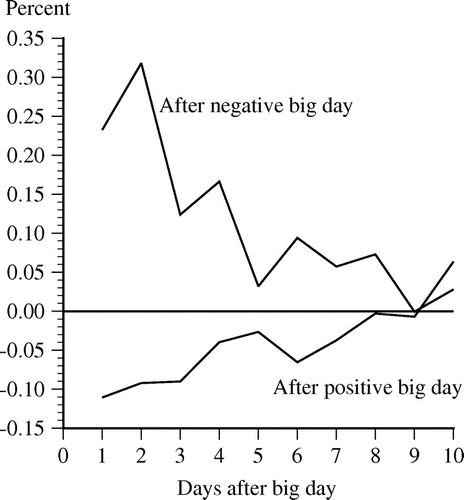
Figure 2. Cumulative average daily adjusted return after a 5% big day.

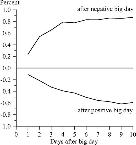
There seems to be a more excessive overreaction to negative events in that the return reversals are, on average, larger following big negative days than big positive days, which is consistent with the asymmetry reported by De Bondt and Thaler (1985). Perhaps this has something to do with the loss aversion documented by Kahneman and Tversky (1984) and Tversky and Kahneman (1991). Overreaction is more pronounced for bad news than for good news, because investors are more susceptible to panic than lust.

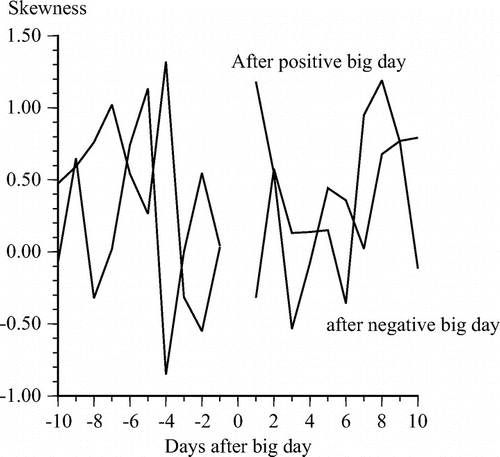
Figure 3 shows the standard deviations of the daily returns for the 10 days preceding and following five-percent big days. These standard deviations increase shortly before big days and fall back afterward, particularly following positive big days. Figure 4 shows the kurtosis of the returns before and after big days. As with the standard deviations, fat tails increase before big days and decline afterward. Figure 5 shows no pattern in the skewness coefficients. The most salient change in the return distribution is that the means are negative for several days after positive big days and positive for several days after negative big days.

Figure 3. Standard deviation of daily adjusted returns before and after a 5% big day.

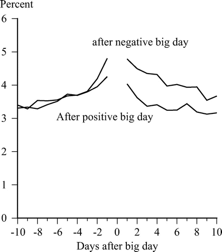
Figure 4. Kurtosis of daily adjusted returns before and after a 5% big day.

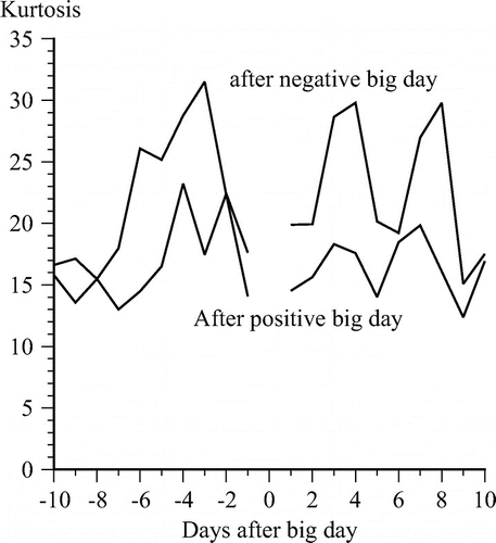
Figure 5. Skewness of daily adjusted returns before and after a 5% big day.

6. Conclusion

There is considerable evidence, in a variety of contexts, that people overreact to recent events, overweighting the importance of new information relative to previous information. This overweighting and overreaction explains why we are so often fooled by regression to the mean in that we do not expect it or recognize it.

Several studies of the stock market have found mean reversion in monthly returns over long horizons, although there are various problems with these studies, including the neglect or possible misspecification of risk premia, which are potentially important over long horizons.

The current paper looks at daily returns on Dow stocks over short horizons, which blunts criticisms that the results are muddled by the neglect of risk premia or the existence of large bid–ask spreads on small, thinly traded stocks, and ensures that the results are not due to the actions of amateur investors. Dow stocks are actively traded with small bid–ask spreads and widely followed by institutional investors. The risk premia on daily returns over short horizons can be safely neglected.

There is strong evidence of overreaction in that large positive and negative returns tend to be followed by persistent, substantial, statistically persuasive reversals over the next 10 days.

Funding

The authors received no direct funding for this research.

Additional information

Notes on contributors

Gary Smith

Gary Smith is Fletcher Jones Professor of Economics at Pomona College. His research encompasses financial markets and statistical reasoning, particularly stock market anomalies and the abuse of data. Several papers debunk fanciful claims, such as Asian-Americans are susceptible to heart attacks on the fourth day of the month; people with positive initials (like ACE) live several years longer than do people with negative initials (like ASS); and people can postpone death until after the celebration of meaningful events, like their birthday, Passover, and the Harvest Moon Festival. He has also explored regression to the mean in a variety of contexts, including testing, sports, business, forecasting, and investing—including the results reported here.

References

- Albuquerque, R. (2012). Skewness in stock returns: reconciling the evidence on firm versus aggregate returns. Review of Financial Studies, 25, 1630–1673.10.1093/rfs/hhr144
- Arbel, A., & Jaggi, B. (1982). Market information assimilation related to extreme daily price jumps. Financial Analysts Journal, 38, 60–66.10.2469/faj.v38.n6.60
- Arora, A., Capp, L., & Smith, G. (2008). The real dogs of the Dow. The Journal of Wealth Management, 10, 64–72.10.3905/jwm.2008.701852
- Beedles, W. L., & Simkowitz, M. A. (1980). Morphology of asset asymmetry. Journal of Business Research, 8, 457–468.10.1016/0148-2963(80)90018-1
- Bland, J. M, & Altman, D. G. (1994). Statistics notes: Some examples of regression towards the mean. British Medical Journal, 309, 780.10.1136/bmj.309.6957.780
- Buffett, W. E. (2008, October). Buy American. I Am. The New York Times, p. 16.
- De Bondt, W. F. M. (1985). Does the stock market overreact to new information? (Unpublished Ph.D. dissertation). Cornell University, Ithaca, NY.
- De bondt, W. F. M., & Thaler, R. (1985). Does the stock market overreact? The Journal of Finance, 40, 793–805.10.1111/j.1540-6261.1985.tb05004.x
- Fama, E. (1965). The behavior of stock-market prices. The Journal of Business, 38, 34–105.10.1086/jb.1965.38.issue-1
- Fama, E. F., & French, K. (1988). Permanent and temporary components of stock prices. Journal of Political Economy, 96, 246–273.10.1086/261535
- Hotelling, H. (1933). The triumph of mediocrity in business. Journal of the American Statistical Association, 28, 463–465.10.2307/2278144
- Kahneman, D., & Tversky, A. (1982). Intuitive prediction: Biases and corrective procedures. In D. Kahneman, P. Slovic, & A. Tversky (Eds.), Judgment under uncertainty. London: Cambridge University Press.10.1017/CBO9780511809477
- Kahneman, D. & Tversky, A. (1984). Choices, values, and frames. American Psychologist, 39(4), 341–350.10.1037/0003-066X.39.4.341
- Keil, M., Smith, G., & Smith, M. (2004). Shrunken earnings predictions are better predictions. Applied Financial Economics, 14, 937–943.10.1080/0960310042000284678
- Kelley, T. L. (1947). Fundamentals of Statistics. Cambridge, MA: Harvard University.
- Keynes, J. M. (1936). The general theory of employment, interest and money (p. 148). London: Macmillan.
- Kim, M. J., Nelson, C., & Startz, R. (1991). Mean reversion in stock prices? A reappraisal of the empirical evidence. The Review of Economic Studies, 58, 515–528.10.2307/2298009
- Lord, Frederic M. & Novick, M. (1968). Statistical Theory of Mental Test Scores. Reading, MA: Addison-Wesley.
- Officer, R. R. (1972). The distribution of stock returns. Journal of the American Statistical Association, 67, 807–812.10.1080/01621459.1972.10481297
- Poterba, J. M., & Summers, L. (1988). Mean reversion in stock prices. Journal of Financial Economics, 22, 27–59.10.1016/0304-405X(88)90021-9
- Richardson, M. (1993). Temporary components of stock prices: A skeptic’s view. Journal of Business and Economic Statistics, 11, 199–207.
- Richardson, M., & Stock, J. (1989). Drawing inferences from statistics based on multiyear asset returns. Journal of Financial Economics, 25, 323–348.10.1016/0304-405X(89)90086-X
- Secrist, H. (1933). The triumph of mediocrity in business. Evanston, IL: Northwestern University.
- Smith, G. (2016). A fallacy that will not die. The Journal of Investing, 25(1), 7–15.10.3905/joi.2016.25.1.007
- Stigler, S. M. (2000). Statistics on the table, the history of statistical concepts and methods (p. 170). Cambridge, MA: Harvard University Press.
- Tversky, A., & Kahneman, D. (1991). Loss aversion in riskless choice: A reference dependent model. QuarterlyJournal of Economics, 107, 1039–1061.
- Zhang, X.-J. (2013). Book-to-market ratio and skewness of stock returns. The Accounting Review, 88, 2213–2240.10.2308/accr-50524