Forecasting USDTRY rate by ARIMA method

Abstract

This paper conducts a USDTRY rate forecast by ARIMA method using 3,069 daily observations between the dates of 3 January 2005 and 8 March 2017 and generates both long-term and short-term models. Existing works related to USDTRY rate forecast using ARIMA method generate static models, and none of them conduct multi-step prediction or out of sample fit. The work described in this paper, however, applies dynamic model generation and conducts multi-step ahead prediction for out of sample observations. In forecasts performed in this work for USDTRY rate, the short-term ARIMAs outperform the long-term ARIMAs in predicting accuracy. Specifically, for the short-term ARIMAs appropriate specification is raised as ARIMA (2,1,0); on the other hand, for the long-term ARIMAs, the best order is emerged as ARIMA (0,1,1).

Keywords:

• ARIMA
• USDTRY
• forecast

Public Interest Statement

Being a candidate country to the European Union and being an emerging economy at the same time, Turkey is a hub for all the investors around the world, especially for the Europeans. In this respect, predictability of Turkish lira has a vital importance to them. Considering these challenges, we try to predict exchange rate of USDTRY by one of the best-known time series forecasting method, namely ARIMA. This work is the sixth of the researches which dealt with USDTRY rate forecasting by ARIMA method. Moreover, the paper is the second study which is written in English in this field. By this way, we bring academic community in current Turkish literature written in this subject. Besides, this study suggests using dynamic and renewed models for every step prediction instead of using static models only, for ARIMA method.

1. Introduction

Foreign exchange rate determines the price of a currency unit, relative to another currency unit. Because every international economic transaction necessitates using foreign currency, it is vital to predict future values of exchange rate for almost every economic agent, especially for the corporations and the governments.

It is also important for a trader to predict the future values of an exchange rate as foreign exchange rates are traded in Foreign Exchange Markets (FXs) with the intention of gaining profit. The idea in this practice is simple, buying low and selling high.

One of the methods for predicting future values of exchange rate is using time series analysis. In their seminal work, Box and Jenkins (1970) identify a procedure for time series forecasting, namely autoregressive integrated moving average (ARIMA) approach which includes model identification, parameter estimation and model checking.

On the other hand, as it is stated by the studies of Zhang (2003) and Pai and Lin (2005), there are limitations of ARIMA method such as pre-assumed linear form of the model. As it is specifically argued by Zhang (2003), the approximation of linearity does not give satisfactory conclusions for real-world problems, in other words ARIMA cannot properly account for the non-linear patterns of data. This means, when ARIMA method is implied in highly volatile time series, forecasting results can lack of accuracy. Considering this drawback, hybrid models such as combination of ARIMA and artificial neural network (ANN) is proposed because of their capabilities of fitting non-linear data better than ARIMA method. Such hybrid models contain ability of machine learning methods (MLM) to be applied in non-linear data.

Although the latest study of Hsu, Lessmann, Sung, Ma, and Johnson (2016) discuss the supremacy of MLM (such as ANN and support vector machines) over econometric methods (EM) (such as ARIMA or generalized autoregressive conditional heteroskedasticity—GARCH) in time series prediction, and conclude with investigating 30 researches done not only in FX markets but also in other financial markets that the best MLM outperform the best EM, the work of Babu and Reddy (2015) shows up as an exception. They conclude that ARIMA model surpasses ANN and fuzzy neuron (FN) in predicting Indian rupee against the major currencies. Hence, as it is highlighted by the study of Babu and Reddy (2015), ARIMA method has still a significance in applying on exchange rates.

In this framework, while being aware of the limitation of linearity assumption for ARIMA method, we aim to forecast United State dollar/Turkish lira (USDTRY) rate using observations between the dates of 3 January 2005 and 8 March 2017 and to forecast both long- and short-term pattern using 3,039 daily observations for long-term models (LTM) and using 119 daily observations for short-term models (STM).

The rest of the paper is organized as follows. Section 2 reviews the current literature about USDTRY rate and about other exchange rate forecasting which use ARIMA method, Section 3 briefly explain the ARIMA method, Section 4 analyses the data by making necessary transformation of the series and by conducting required tests, Section 5 analyse and ensure the stationary condition, Section 6 specifies the models and makes predictions, Section 7 discusses the results and, finally, Section 8 provides the conclusion.

2. Related works

2.1. Related works for USDTRY rate forecasting using ARIMA method

To the best of our knowledge there are few studies related to USDTRY rate forecasting using ARIMA method.

Bircan and Karagoz (2003) analyse monthly average price of USDTRY using 132 monthly observations between the date of January 1991 and December 2002. They estimate an ARIMA model with (2,1,1) order and conclude that ARIMA method is appropriate for USDTRY forecasting.

Kadilar, Şimşek, and Aladağ (2009) find the most appropriate model as ARIMA (0,0,1) (0,0,1)6 using weekly rates of USDTRY between the dates of 3 January 2005 and 28 January 2008 with 160 observations.

Vergil and Özkan (2007) compare the success of ARIMA model against monetary model (MM) by fitting the USDTRY rate with the monthly observations taken from the dates between January 1980 and July 2001. By reaching ARIMA (3,1,2) as the appropriate specification, they conclude ARIMA is more efficient in fitting USDTRY rate compared to MM.

Kaynar and Taştan (2009), taking the observations both daily and monthly between the dates of January 2000 and June 2008 find the best model for the former as ARIMA (2,1,0) and for the later as ARIMA (0,1,1).

Özkan (2011), using 338 monthly observations for the years of 1986 and 2010 compares three model including ARIMA, ANN and conjunctural model (CM). Although, she does not state the specification of generated ARIMA model, concludes that ANN is the most successful method for predicting USDTRY rate.

None of the literature specified above, however, makes one or multi step ahead prediction for out of sample observations. On the contrary, they just evaluate the generated models with the observations used also for generating the model.

2.2. Related works for other currency rates forecasting using ARIMA method

Yao and Tan (2000), using observations of 510 weekly closing rates of United State dollar/Japanese yen (USDJPY), United State dollar/Deutsche mark (USDDM), United State dollar/British pound (USDGBP), United State dollar/Swiss franc (USDCHF), United State dollar/Australian dollar (USDAUD) between the dates of 18 May 1984 and 7 of July 1995, investigate if ANN predictions are applicable for gaining FX trading profits.

They generate two different ANN models, one with delay variables of the currency as input variables and the other with technical indicators as input variables. By conducting this analysis, they also compare ARIMA models with these two ANN models and conclude that ANN outperforms ARIMA.

Zhang (2003) creates a hybrid model of ARIMA and ANN. Using this hybrid model and 731 weekly observations from 1980 to 1993, he forecasts USDGBP rate and deduces that hybrid model gives more sound results than both ARIMA and ANN.

Maniatis (2012), using 3,202 daily observations between the dates of 4 of January 1999 and 1 July 2011 forecasts European Union currency/United State dollar (EURUSD) rate by ARIMA method, exponential smoothing technique (EST) and probabilistic approach (PA). He concludes that the latter outperforms the others.

Maria and Eva (2011), forecast exchange rates of European Union currency/Romanian leu (EURRON), United State dollar/Romanian leu (USDRON), British pound/Romanian leu (GBPRON), Japanese yen/Romanian leu (JPYRON), Chinese yuan/Romanian leu (CNYRON), Russian ruble/Romanian leu (RUBRON) using 80 daily observations taken from 3 January 2011 and 22 April 2011 with ARIMA method and EST. They find the appropriate models as ARIMA (1,0,0) for EURRON, ARIMA (1,0,0) for USDRON, ARIMA (1,1,1) for GBPRON, ARIMA (4,0,6) for JPYRON, ARIMA (1,0,0) for CNYRON, ARIMA (1,1,3) for RUBRON. However, the authors conclude that EST gives more significant results than ARIMA.

Nwankwo (2014), with using yearly average values of Nigerian naira/United State dollar (NGNUSD) between the years of 1982 and 2011, find ARIMA (1,0,0) is suitable for forecasting of NGNUSD.

Babu and Reddy (2015) compare the methods of ARIMA, ANN and fuzzy systems on 1,284 daily observations of United State dollar/Indian rupee (USDINR), British pound/Indian rupee (GBPINR), European Union currency/Indian rupee (EURINR), Japanese yen/Indian rupee (JPYINR) between the dates of January 2010 and April 2015. They generate models of ARIMA (1,1,0), ARIMA (0,1,1), ARIMA (1,1,1), ARIMA (2,1,0), ARIMA (0,1,2) and ARIMA (2,1,2) respective to mentioned exchange rates, and conclude that ARIMA gives more significant results than ANN and fuzzy systems.

3. ARIMA method

In able to forecast a time series, stationarity must be fulfilled. Required conditions for a weakly stationary time series are a time-independent mean, $E(z_t)=\mathit{\mu }$, and a constant variance between the consecutive observations, $\text{Cov}\left(z_t,z_{t-\mathit{\iota }}\right)={\mathit{\gamma }}_{\mathit{\iota }}$.(1) $$z_t={\mathit{\varphi }}_1{z}_{t-1}+\cdots +{\mathit{\varphi }}_p{z}_{t-p}+a_t\Rightarrow z_t=\mathit{\varphi }{(B)}^{-1}{a}_t$$(1) (2) $$z_t=a_t-{\mathit{\theta }}_1{a}_{t-1}-\cdots -{\mathit{\theta }}_q{a}_{t-q}\Rightarrow z_t=\mathit{\theta }(B)a_t$$(2) (3) $$z_t={\mathit{\varphi }}_1{z}_{t-1}+\cdots +{\mathit{\varphi }}_p{z}_{t-p}+a_t-{\mathit{\theta }}_1{a}_{t-1}-\cdots -{\mathit{\theta }}_q{a}_{t-q}\Rightarrow z_t=\frac{\mathit{\theta }(B)}{\mathit{\varphi }(B)}{a}_t$$(3)

where p—parameter autoregressive AR(p) model can be illustrated as (1), while q—parameter moving average MA(q) model can be formulized as (2), thus an ARMA (p, q) model can be represented as (3).(4) $$\mathit{\varphi }(B){\mathrm{\nabla }}^d{z}_t={\mathit{\theta }}_0+\mathit{\theta }(B)a_t$$(4)

If original series is not stationary, transformation such as differencing should be applied. If stationary is ensured after differencing at series’ first level this means the original series has one unit root. This is defined as I (1), for levels more than 1 it is defined as “d”. In this case, the model specification is stated as ARIMA (p, d, q) as (4).

4. Data

4.1. Descriptive statistics

Original data are taken from the web site of Central Bank of Turkey (CBRT). The data include 3,069 observations of daily ask price of USDTRY between the dates of 3 January 2005 and 8 March 2017.

A total of 3,069 observations are used generating the LTM and the subsample (2,921 and 3,069th) of the total data are used generating the STM.

On the propose of performing routine time series transformation we follow these steps; original series (Price of USDTRY) is represented as P_t, natural logarithm of the price is taken as lnP_t and natural logarithmic return is transformed as r_t = lnP_t − lnP_t + 1. Because, we aim to generate two different models as LTM and STM, six different series are created, namely P_(LTM)t, lnP_(LTM)t, r_(LTM)t, P_(STM)t, lnP_(STM) and r_(STM)t (Table 1).

Table 1. Descriptive statistics for P_(LTM)t and P_(STM)t

	P(LTM)t	P(STM)t
Minimum	1.150	2.928
1st quarter	1.408	3.020
Median	1.605	3.388
Mean	1.845	3.343
3rd quarter	2.122	3.622
Maximum	3.885	3.885

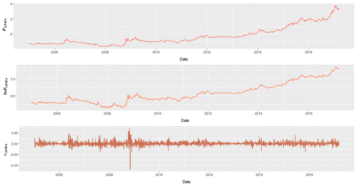
Figure 1 depicts the graph of LTM series against time. For, P_(LTM)t clear up trend is apparent starting from the third quarter of 2008 to beginning of 2017. After, taking natural logarithm of the P_(LTM)t, the range between the first value and the last value is got smaller. r_(STM)t series; on the other hand, shows a random behaviour with volatility clustering.

Figure 1. Time plots of P_(LTM)t, lnP_(LTM)t, r_(LTM)t.

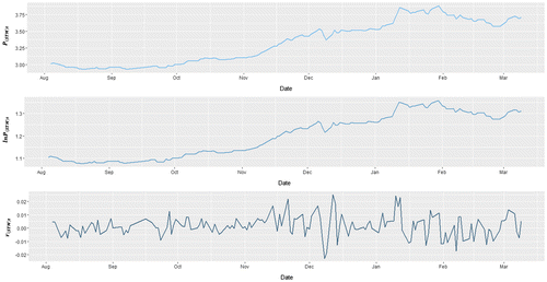
Figure 2 demonstrates the graph of STM series against time. There is also a rising trend with the beginning of October 2016 through the 2017 for P_(STM)t. As for r_(STM)t, volatility is also observable.

Figure 2. Time plots of P_(STM)t, lnP_(STM)t, r_(STM)t.

5. Stationarity

To examine stationarity augmented Dickey–Fuller (ADF) (Dickey & Fuller, 1981) test is performed for the series of LTM and STM. Because P_t and lnP_t series of both LTM and STM show a clear uptrend, trend parameter is added to ADF Equations (5), however, test of ADF for r_t series of both LTM and STM executed with unit root model (6).(5) $$\mathrm{\nabla }{y}_t=\mathit{\delta }{y}_{t-1}+a_0+a_{1}t+u_t$$(5) (6) $$\mathrm{\nabla }{y}_t=\mathit{\delta }{y}_{t-1}+u_t$$(6)

Hypotheses are created as follows: “H₀ = The series is stationary” and the alternative, “H_a = The series is not stationary”, considering Table 2. As for P_(LTM)t, lnP_(LTM)t, P_(STM)t and lnP_(STM)t, because a₁ values of the models greater than the “DF test statistics”, null hypothesis is rejected. While, because δ values of r_(LTM)t and r_(STM)t are bigger than “DF test statistics” in absolute values null hypothesis are not rejected that implies r_(LTM)t and r_(STM)t are stationary. After stationarity is ensured for both lnP_(LTM)t and lnP_(STM)t at their first differences as r_(LTM)t and r_(STM)t series, modelling is performed.

Table 2. ADF test for LTM and STM series

	α1	δ	DF test statistics
P(LTM)t	6.250	x	3.7097
lnP(LTM)t	6.250	x	3.2998
r(LTM)t	x	−1.950	−24.9135
P(STM)t	6.490	x	2.3484
lnP(STM)t	6.490	x	2.3649
r(STM)t	x	−1.950	−4.6889

6. Model specification and application

There are various ways of order determination suggested in the literature. However, these methods are mostly subjective. In other words, for the same data, different diagnostic methods determinate different order numbers. Considering this drawback, a trial and error learning approach is adopted, hence both for lnP_(LTM)t and lnP_(STM)t, 30 renewed models of ARIMA (1,1,0), ARIMA (2,1,0), ARIMA (0,1,1), ARIMA (0,1,2), ARIMA (1,1,1), ARIMA (2,1,1), ARIMA (1,1,2) and ARIMA (2,1,2) are generated in a dynamic manner.

Straightforwardly, the first LTM is generated using the observations between 1st and 3,040th for predicting 3,041st value and, by following the same practice, the last LTM is generated using the observation between 30th and 3,069th for predicting 3,070th value. The same dynamic manner is performed for STMs. For the first STM with the intention of predicting 3,041st value, observations between 2,921st and 3,040th are used and by following the same practice again, for the last STM with the aim of predicting 3,070th value, observations between 2,960th and 3,069th are used.

To find best-performing model, a simple method, namely average absolute deviations is applied. Thus, predicted values of the series subtracted from the actual value in the absolute value operator and divided to 30. Results of this process are interpreted as “the minimum valued model outperforms the other models”.(7) $$\frac{1}{n}\sum _{i=1}^n\left|P_{(\text{actual})t}-P_{(\text{predicted})t}\right|$$(7)

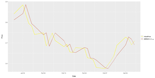
Table 3 suggests ARIMA (0,1,1)_LTM is the best-performing model among eight models. Figure 3 depicts the performance of ARIMA (0,1,1)_LTM by graphing predicted values relative to actual values of USDTRY rate between the dates of 27 of January in 2017. All the predictions made by LTMs versus actual price (AP) can be found at Appendix 1.

Table 3. Absolute means for LTMs

	Average absolute deviations
ARIMA (1,1,0)LTM	0.02679088
ARIMA (0,1,1)LTM	0.02678898
ARIMA (2,1,0)LTM	0.02681889
ARIMA (0,1,2)LTM	0.02681356
ARIMA (1,1,1)LTM	0.02680419
ARIMA (1,1,2)LTM	0.02680568
ARIMA (2,1,1)LTM	0.02683304
ARIMA (2,1,2)LTM	0.02685333

Figure 3. ARIMA (0,1,1)_LTM predictions vs. actual price.

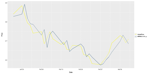
On the other hand, for the STMs, according to Table 4 ARIMA (0,1,1)_STM accounts for the minimum value of average absolute deviation, which means ARIMA (2,1,0)_STM is the best model. Figure 4 reflects actual values related to predicted values of ARIMA (2,1,0)_STM. All the predictions made by STMs versus AP can be found at Appendix 2.

Table 4. Absolute means for STMs

	Average absolute deviations
ARIMA (1,1,0)STM	0.026642835
ARIMA (0,1,1)STM	0.026490678
ARIMA (2,1,0)STM	0.026083231
ARIMA (0,1,2)STM	0.026096396
ARIMA (1,1,1)STM	0.026223956
ARIMA (1,1,2)STM	0.02610454
ARIMA (2,1,1)STM	0.026228585
ARIMA (2,1,2)STM	0.02650923

Figure 4. ARIMA (2,1,0)_STM predictions vs. actual price.

7. Results and discussion

In study of Yao and Tan (2000) which concludes that results of ANN models are better than ARIMA models, ARIMA (1,0,1) and ARIMA (2,0,2) of USDJPY, USDDM, USDGBP, USDCHF, USDAUD rates are generated. However, it is not indicated whether the data are stationary or not.

Zhang (2003) executes forecasts of 1, 6 and 12 months for GBPUSD observations, in both time horizons hybrid model is better than ANN and ARIMA. They find that best ARIMA model for GBPUSD model is random walk.

In the study of Kaynar and Taştan (2009), it is found that ARIMA (2,1,0) is suitable for daily data which are taken between the dates of January 2000 and June 2008. This is not coincide with our study as it states the best model of long term is ARIMA (0,1,1).

Steve (2012), finds that ARIMA (1,0,0) is appropriate model for NGNUSD rate in the period between 1982 and 2011, without indicating type of the observation (daily or weekly) and without performing any prediction.

The work of Maria and Eva (2011) worth comparing with our study, as it investigates currency of a developing country, namely Romania. They find the best specification for RONUSD as ARIMA (1,0,0) model. Because, the study considers 80 daily observations, the model can be specified as short term. In this regard, we can compare it our best-performing STM which is ARIMA (2,1,0)_STM. What is interesting about Maria & Eva’s model for RONUSD is that their model’s p-value is 0.

The research of Babu and Reddy (2015) is interesting for two aspects. Firstly, because India resembles in Turkey for its being an emerging market. Secondly, their study concludes that being a linear model ARIMA surpasses non-linear methods such as ANN and FN. When we compared their study with ours, it can be said that with 1,284 observations their ARIMA model come right in the middle of our STM (109 observations) and LTM (3,039 observations). They conclude that ARIMA (1,1,1) is the best for modelling USDINR, GBPINR and JPYINR and ARIMA (1,1,0) is the best for modelling EURINR.

Professionals such as traders, financial managers and policy-makers often need to foresee value of exchange rates for deciding trade activities, hedging their liabilities and planning public policy. In this context, they rely on various forecasting methods.

Although when the results of this study are compared to the literature dealt with exchange rate forecasting by ARIMA method some differences observed, this study reveals that while using ARIMA method, professionals should consider that there is a tendency for short-term models to produce more sound results than long-term models for exchange rate prediction.

Besides, this study suggests using dynamic and renewed models for every step prediction instead of using static models only, for ARIMA method.

8. Conclusion

Using daily values of USDTRY rate, eight different ARIMA models are generated in a dynamic manner with 30 renewed (hence updated) models for both LTM and STM. Among these models the predictions sets of 30 renewed ARIMA (0,1,1)_LTM models have performed better, for STMs, however, predictions made by 30 renewed sets of ARIMA (2,1,0)_STM outperformed the others.

Moreover, ARIMA (2,1,0)_STM has showed better performance than ARIMA (0,1,1)_LTM. This means ARIMA method is more effective in short-term prediction for USDTRY rate.

Funding

The authors received no direct funding for this research.

Additional information

Notes on contributors

Cenk Ufuk Yıldıran

Cenk Ufuk Yıldıran did BSc in Econometrics at Istanbul University, 2007. He has been awarded the Jean Monnet Scholarship in 2013; by this way, he studied MSc in Economics and Econometrics at the University of Essex, 2014, and also completed his MSc in Finance in Kocaeli University, 2017. He has been working as a European Union expert at the Ministry of Science, Industry and Technology of Turkey since 2009.

Abdurrahman Fettahoğlu

Abdurrahman Fettahoğlu has graduated from Marmara University in 1973. He completed his MBA in 1977 and PhD in Finance in 1980, in Wirtschaftsuniversität Wien University. He worked as an assistant professor in 1983 and 1985 in Karedeniz Technical University. He received the title of professor in 1993 from Kocaeli University. Between the years of 2006 and 2013, he has served as dean of faculty of economics and administrative sciences at Kocaeli University. He is currently working at Kocaeli University as professor doctor.

Appendix 1

Predictions made by STMs

Table

Date	AP	AR1	MA1	AR2	MA2	AR1MA1	AR1MA2	AR2MA1	AR2MA2
1.27.2017	3.84120	3.81147	3.81146	3.81135	3.81137	3.81110	3.81108	3.81120	3.81062
1.30.2017	3.88480	3.84191	3.84187	3.84238	3.84233	3.84120	3.84266	3.84230	3.84245
1.31.2017	3.83930	3.88592	3.88588	3.88618	3.88612	3.88590	3.88613	3.88616	3.88648
2.1.2017	3.79420	3.83816	3.83815	3.83851	3.83846	3.83816	3.83847	3.83850	3.83913
2.2.2017	3.78140	3.79305	3.79309	3.79278	3.79282	3.79307	3.79282	3.79280	3.79284
2.3.2017	3.74040	3.78107	3.78110	3.78079	3.78085	3.78108	3.78084	3.78081	3.78066
2.6.2017	3.74890	3.73933	3.73935	3.73925	3.73929	3.73934	3.73928	3.73926	3.73905
2.7.2017	3.68510	3.74912	3.74915	3.74884	3.74889	3.74913	3.74888	3.74885	3.74874
2.8.2017	3.71620	3.68345	3.68347	3.68353	3.68355	3.68346	3.68355	3.68354	3.68333
2.9.2017	3.74780	3.71699	3.71702	3.71649	3.71655	3.71701	3.71654	3.71650	3.71643
2.10.2017	3.71140	3.74861	3.74858	3.74883	3.74881	3.74860	3.74881	3.74883	3.74870
2.13.2017	3.68150	3.71049	3.71048	3.71071	3.71068	3.71049	3.71069	3.71071	3.71085
2.14.2017	3.69350	3.68074	3.68077	3.68052	3.68056	3.68075	3.68055	3.68056	3.68055
2.15.2017	3.65600	3.69381	3.69383	3.69363	3.69367	3.69336	3.69344	3.69364	3.69352
2.16.2017	3.65280	3.65505	3.65505	3.65513	3.65514	3.65505	3.65514	3.65514	3.65500
2.17.2017	3.67700	3.65272	3.65274	3.65248	3.65252	3.65273	3.65251	3.65249	3.65239
2.20.2017	3.67280	3.67762	3.67761	3.67760	3.67760	3.67762	3.67760	3.67759	3.67728
2.21.2017	3.62770	3.67269	3.67268	3.67283	3.67281	3.67269	3.67281	3.67283	3.67276
2.22.2017	3.62510	3.62655	3.62656	3.62653	3.62654	3.62655	3.62654	3.62653	3.62654
2.23.2017	3.61690	3.62503	3.62506	3.62480	3.62485	3.62505	3.62484	3.62481	3.62475
2.24.2017	3.58110	3.61669	3.61669	3.61668	3.61669	3.61669	3.61669	3.61668	3.61638
2.27.2017	3.57530	3.58018	3.58020	3.58015	3.58016	3.58019	3.58016	3.58016	3.57990
2.28.2017	3.59460	3.57515	3.57517	3.57498	3.57502	3.57516	3.57501	3.57508	3.57460
3.1.2017	3.61430	3.59512	3.59512	3.59509	3.59510	3.59493	3.59514	3.59487	3.59447
3.2.2017	3.63780	3.61484	3.61482	3.61488	3.61486	3.61481	3.61463	3.61488	3.61487
3.3.2017	3.68820	3.63843	3.63841	3.63850	3.63847	3.63842	3.63848	3.63849	3.63860
3.6.2017	3.72820	3.68960	3.68957	3.68969	3.68965	3.68958	3.68966	3.68967	3.69015
3.7.2017	3.71810	3.72934	3.72929	3.72949	3.72941	3.72903	3.72924	3.72944	3.72978
3.8.2017	3.69080	3.71781	3.71778	3.71794	3.71788	3.71779	3.71790	3.71832	3.71831
3.9.2017	3.70970	3.69003	3.69004	3.69000	3.69001	3.69012	3.69003	3.69024	3.69081

Appendix 2

Predictions made by LTMs

Table

Date	AP	AR1	MA1	AR2	MA2	AR1MA1	AR1MA2	AR2MA1	AR2MA2
1.27.2017	3.84120	3.82281	3.82738	3.82839	3.82381	3.82435	3.82463	3.82650	3.82665
1.30.2017	3.88480	3.84896	3.84590	3.84014	3.84217	3.84385	3.84185	3.83949	3.83866
1.31.2017	3.83930	3.89611	3.89822	3.89229	3.89652	3.89747	3.89590	3.89419	3.89410
2.1.2017	3.79420	3.82866	3.82083	3.81796	3.81971	3.82019	3.81887	3.81803	3.81869
2.2.2017	3.78140	3.78293	3.78563	3.79007	3.79272	3.79040	3.79192	3.79052	3.79020
2.3.2017	3.74040	3.77817	3.77993	3.78676	3.78037	3.77931	3.78174	3.78645	3.78727
2.6.2017	3.74890	3.72993	3.72664	3.73036	3.72915	3.72849	3.72935	3.72887	3.72909
2.7.2017	3.68510	3.75103	3.75649	3.75935	3.75892	3.75786	3.75962	3.75950	3.75997
2.8.2017	3.71620	3.66953	3.66255	3.66545	3.66220	3.66179	3.66253	3.66425	3.66409
2.9.2017	3.74780	3.72312	3.73051	3.73437	3.73540	3.73441	3.73533	3.73429	3.73167
2.10.2017	3.71140	3.75512	3.75262	3.75111	3.74633	3.74698	3.74772	3.75119	3.75368
2.13.2017	3.68150	3.70354	3.69936	3.69671	3.70172	3.70365	3.70085	3.69721	3.69804
2.14.2017	3.69350	3.67479	3.67619	3.68010	3.67968	3.67790	3.67984	3.68071	3.68078
2.15.2017	3.65600	3.69619	3.69890	3.70237	3.69942	3.69886	3.69990	3.70172	3.70211
2.16.2017	3.65280	3.64767	3.64312	3.64411	3.64318	3.64295	3.64328	3.64306	3.64309
2.17.2017	3.67700	3.65209	3.65556	3.65831	3.65950	3.65851	3.65947	3.65901	3.65909
2.20.2017	3.67280	3.68242	3.68349	3.68397	3.68056	3.68059	3.68127	3.68270	3.68259
2.21.2017	3.62770	3.67187	3.66958	3.66743	3.66896	3.66977	3.66868	3.66731	3.66743
2.22.2017	3.62510	3.61774	3.61488	3.61665	3.61762	3.61667	3.61736	3.61721	3.61724
2.23.2017	3.61690	3.62453	3.62818	3.63274	3.63146	3.63004	3.63172	3.63289	3.63293
2.24.2017	3.58110	3.61509	3.61348	3.61523	3.61235	3.61213	3.61286	3.61374	3.61367
2.27.2017	3.57530	3.57319	3.57113	3.57321	3.57434	3.57364	3.57416	3.57340	3.57327
2.28.2017	3.59460	3.57402	3.57658	3.58020	3.57886	3.57758	3.57919	3.58018	3.58029
3.1.2017	3.61430	3.59888	3.60022	3.60075	3.59872	3.59886	3.59908	3.59933	3.59924
3.2.2017	3.63780	3.61872	3.61871	3.61593	3.61680	3.61766	3.61679	3.61593	3.61582
3.3.2017	3.68820	3.64308	3.64379	3.64041	3.64181	3.64274	3.64166	3.64129	3.64126
3.6.2017	3.72820	3.69999	3.70242	3.69779	3.69907	3.70032	3.69895	3.69872	3.69876
3.7.2017	3.71810	3.73800	3.73657	3.73074	3.73232	3.73383	3.73201	3.73132	3.73144
3.8.2017	3.69080	3.71571	3.71209	3.70812	3.71135	3.71224	3.71065	3.70984	3.71011
3.9.2017	3.70970	3.68424	3.68379	3.68487	3.68620	3.68557	3.68581	3.68623	3.68666

References

- Babu, A. S., & Reddy, S. K. (2015). Exchange rate forecasting using ARIMA, neural network and fuzzy neuron. Journal of Stock & Forex Trading, 3(4), 1–5. doi:10.4172/2168-9458.1000155
- Bircan, H., & Karagoz, Y. (2003). Box Jenkins Modelleri İle Aylık Döviz Kuru Tahmini Üzerine Bir Uygulama. Kocaeli Üniversitesi Sosyal Bilimler Enstitüsü Dergisi, 6, 49–62. Retrieved from http://dergipark.gov.tr/download/article-file/252067
- Box, G. E., & Jenkins, G. M. (1970). Time series analysis, forecasting, and control. San Francisco, CA: Holden - Day.
- Dickey, D. A., & Fuller, W. A. (1981). Likelihood ratio statistics for autoregressive time series with a unit root. Econometrica, 1057–1072. Retrieved from http://www.jstor.org/stable/191251710.2307/1912517
- Hsu, M. W., Lessmann, S., Sung, M. C., Ma, T., & Johnson, J. E. (2016). Bridging the divide in financial market forecasting: Machine learners vs. financial economists. Expert Systems with Applications, 61, 215–234. doi:10.1016/j.eswa.2016.05.033
- Kadilar, C., Şimşek, M., & Aladağ, A. G. Ç. H. (2009). Forecasting the exchange rate series with ANN: The case of Turkey. Ekonometri ve İstatistik e-Dergisi, 9, 17–29. Retrieved from http://www.journals.istanbul.edu.tr/iuekois/article/view/1023005311
- Kaynar, O., & Taştan, S. (2009). Zaman Serisianalizinde MLP Yapay Sinir Ağları Ve Arıma Modelinin Karşılaştırılması. Erciyes Üniversitesi İktisadi ve İdari Bilimler Fakültesi Dergisi, (33), 161–172. Retrieved from http://iibf.erciyes.edu.tr/dergi/sayi33/9.k%C4%B1s%C4%B1m.pdf
- Maniatis, P. (2012). Forecasting the exchange rate between Euro and USD: Probabilistic approach versus ARIMA and exponential smoothing techniques. Journal of Applied Business Research (JABR), 28, 171–192. doi:10.19030/jabr.v28i2.6840
- Maria, F. C., & Eva, D. (2011). Exchange-rates forecasting: exponential smoothing techniques and ARIMA models. Annals of Faculty of Economics, 1, 499–508. Retrieved from http://anale.steconomiceuoradea.ro/volume/2011/n1/046.pdf
- Nwankwo, S. C. (2014). Autoregressive integrated moving average (ARIMA) model for exchange rate (Naira to Dollar). Academic Journal of Interdisciplinary Studies, 3, 429. doi:10.5901/ajis.2014.v3n4p42
- Özkan, F. (2011). Döviz Kuru Tahmininde Yapay Sinir Ağlarıyla Alternatif Yaklaşım. Eskişehir Osmangazi Üniversitesi, İİBF Dergisi, (s 6), 2. Retrieved from http://iibfdergi.ogu.edu.tr/makaleler/11352029_6_6-2_Makale_0.pdf
- Pai, P. F., & Lin, C. S. (2005). A hybrid ARIMA and support vector machines model in stock price forecasting. Omega, 33, 497–505. doi:10.1016/j.omega.2004.07.024
- Vergil, H., & Özkan, F. (2007). Döviz Kurları Öngörüsünde Parasal Model ve Arima Modelleri: Türkiye Örneği. Retrieved from http://dergipark.gov.tr/kosbed/issue/25707/271265
- Yao, J., & Tan, C. L. (2000). A case study on using neural networks to perform technical forecasting of forex. Neurocomputing, 34, 79–98. doi:10.1016/S0925-2312(00)00300-3
- Zhang, G. P. (2003). Time series forecasting using a hybrid ARIMA and neural network model. Neurocomputing, 50, 159–175. doi:10.1016/S0925-2312(01)00702-0