A simulation study on the distributions of disturbances in the GARCH model

Abstract

Generalized autoregressive conditional heteroskedastic (GARCH) model is a standard approach to study the volatility behaviour of financial time series. The original specification of GARCH model is developed based on Normal distribution for the disturbances, which cannot accommodate fat-tailed properties commonly existing in financial time series. Consequently, the resulting estimates are not efficient. Traditionally, the Student’s t-distribution and General Error Distribution (GED) are used alternatively to solve this problem. However, a recent study points out that those alternative distributions lack stability under aggregation. This leaves the appropriate choice of the distribution of disturbances in the GARCH model still an open question. In this paper, we present the theoretical features and desirability of the tempered stable distribution. Further, we conduct a series of simulation studies to demonstrate that the GARCH model with this distribution consistently outperforms those with the Normal, Student-t and GED distributions. This result is robust with empirical evidence of the S&P 500 daily return. Therefore, we argue that the tempered stable distribution could be a widely useful tool for modelling the financial volatility in general contexts with a GARCH-type specification.

Keywords:

• GARCH model
• disturbances
• fat-tailed distribution
• tempered stable distribution

Public Interest Statement

This paper provides a systematic and comprehensive investigation on the distributions of disturbances in the Generalized autoregressive conditional heteroskedastic (GARCH) model. This model is derived based on the seminal work of the Nobel laureate Robert Engle and has been widely used in finance research in the past few decades. Its application covers many fields including financial volatility forecasting and quantitative risk management. With both simulation and empirical evidence, we demonstrate that the tempered stable distribution outperforms other popular existing options including Gaussian, Student’s t and gender error distributions. Hence, via incorporating the tempered stable distribution, the accuracy of the GARCH model can be largely increased. Further, the practical implication of such a model is expected to be more appropriate, which benefits users like stock market traders and relevant policy markers.

1. Introduction

Over the past few decades, the autoregressive conditional heteroskedastic (ARCH) model has become a standard approach to study the volatility of financial time series. This framework is firstly proposed by Engle (1982) and is further extended to be the generalized ARCH (GARCH) model (Bollerslev, 1986). The popularity of GARCH model is particularly due to its ability to capture characteristics of financial time series like time varying heteroskedasticity and volatility clustering (Ho, Shi, & Zhang, 2013).

Table 1. Simulation results: Student’s t-distribution

$\mathit{\alpha }$	$\mathit{\beta }$	T	${\text{Mean}}_{ll}$	${\text{Bias}}_{\mathit{\alpha }}$	${\text{SE}}_{\mathit{\alpha }}$	${\text{RMSE}}_{\mathit{\alpha }}$	${\text{Bias}}_{\mathit{\beta }}$	${\text{SE}}_{\mathit{\beta }}$	${\text{RMSE}}_{\mathit{\beta }}$	${\text{Bias}}_{\mathit{\alpha }+\mathit{\beta }}$	${\text{SE}}_{\mathit{\alpha }+\mathit{\beta }}$	${\text{RMSE}}_{\mathit{\alpha }+\mathit{\beta }}$
Panel A: Normal distribution
0.10	0.65	3,000	$-2,708$	0.0219	0.1211	0.1231	$-0.0481$	0.1998	0.2055	$-0.0262$	0.1605	0.1626
		4,000	$-3,614$	0.0207	0.1125	0.1144	$-0.0448$	0.1719	0.1776	$-0.0241$	0.1352	0.1374
		5,000	$-4,493$	0.0132	0.0882	0.0892	$-0.0451$	0.1599	0.1661	$-0.0318$	0.1258	0.1298
0.15	0.70	3,000	$-3,237$	0.0108	0.1052	0.1058	$-0.0386$	0.1339	0.1394	$-0.0278$	0.1063	0.1098
		4,000	$-4,339$	0.0101	0.0963	0.0968	$-0.0166$	0.1188	0.1199	$-0.0065$	0.0765	0.0768
		5,000	$-5,414$	0.0133	0.0884	0.0894	$-0.0345$	0.1137	0.1188	$-0.0212$	0.0791	0.0819
0.20	0.75	3,000	$-4,112$	0.0138	0.1190	0.1198	$-0.0309$	0.1114	0.1156	$-0.0171$	0.0494	0.0523
		4,000	$-5,474$	$-0.0057$	0.0732	0.0734	$-0.0125$	0.0759	0.0770	$-0.0182$	0.0450	0.0485
		5,000	$-6,843$	0.0068	0.0742	0.0745	$-0.0187$	0.0696	0.0721	$-0.0118$	0.0455	0.0470
Panel B: Student’s t-Distribution
0.10	0.65	3,000	$-2,167$	0.0022	0.0272	0.0273	$-0.0045$	0.0826	0.0828	$-0.0023$	0.0686	0.0686
		4,000	$-2,884$	0.0000	0.0228	0.0228	$-0.0029$	0.0708	0.0708	$-0.0029$	0.0600	0.0600
		5,000	$-3,607$	0.0022	0.0205	0.0206	$-0.0070$	0.0560	0.0564	$-0.0048$	0.0469	0.0471
0.15	0.70	3,000	$-2,714$	0.0032	0.0311	0.0313	$-0.0071$	0.0489	0.0494	$-0.0039$	0.0379	0.0381
		4,000	$-3,627$	$-0.0005$	0.0289	0.0289	$-0.0022$	0.0428	0.0429	$-0.0027$	0.0321	0.0322
		5,000	$-4,530$	0.0013	0.0246	0.0247	$-0.0033$	0.0364	0.0366	$-0.0020$	0.0287	0.0288
0.20	0.75	3,000	$-3,570$	0.0045	0.0380	0.0383	$-0.0051$	0.0332	0.0336	$-0.0006$	0.0281	0.0281
		4,000	$-4,760$	0.0005	0.0292	0.0292	$-0.0017$	0.0250	0.0250	$-0.0012$	0.0231	0.0231
		5,000	$-5,949$	0.0004	0.0264	0.0264	$-0.0009$	0.0226	0.0227	$-0.0005$	0.0217	0.0217
Panel C: GED distribution
0.10	0.65	3,000	$-2,216$	$-0.0150$	0.0250	0.0291	$-0.0077$	0.0957	0.0960	$-0.0227$	0.0812	0.0843
		4,000	$-2,948$	$-0.0148$	0.0210	0.0257	$-0.0079$	0.0764	0.0768	$-0.0227$	0.0656	0.0694
		5,000	$-3,687$	$-0.0139$	0.0194	0.0239	$-0.0126$	0.0641	0.0654	$-0.0265$	0.0534	0.0596
0.15	0.70	3,000	$-2,761$	$-0.0225$	0.0269	0.0350	$-0.0100$	0.0544	0.0553	$-0.0325$	0.0411	0.0524
		4,000	$-3,692$	$-0.0244$	0.0259	0.0356	$-0.0024$	0.0489	0.0489	$-0.0268$	0.0351	0.0441
		5,000	$-4,609$	$-0.0226$	0.0211	0.0309	$-0.0081$	0.0422	0.0430	$-0.0307$	0.0322	0.0445
0.20	0.75	3,000	$-3,619$	$-0.0288$	0.0332	0.0439	-0.0077	0.0360	0.0368	$-0.0364$	0.0237	0.0435
		4,000	-4,824	$-0.0329$	0.0245	0.0410	$-0.0032$	0.0296	0.0297	$-0.0361$	0.0196	0.0411
		5,000	$-6,029$	$-0.0312$	0.0229	0.0387	$-0.0029$	0.0260	0.0262	$-0.0341$	0.0173	0.0383
Panel D: Tempered stable distribution
0.10	0.65	3,000	$-2,162$	0.0099	0.0595	0.0604	$-0.0051$	0.0841	0.0843	0.0048	0.0854	0.0856
		4,000	$-2,879$	$-0.0032$	0.0349	0.0350	$-0.0032$	0.0729	0.0729	$-0.0065$	0.0660	0.0663
		5,000	$-3,602$	$-0.0025$	0.0270	0.0271	$-0.0066$	0.0576	0.0579	$-0.0091$	0.0506	0.0514
0.15	0.70	3,000	$-2709$	0.0021	0.0459	0.0460	$-0.0073$	0.0502	0.0507	$-0.0052$	0.0522	0.0524
		4,000	$-3,622$	$-0.0048$	0.0400	0.0403	$-0.0019$	0.0435	0.0435	$-0.0067$	0.0431	0.0436
		5,000	$-4,525$	$-0.0075$	0.0250	0.0261	$-0.0035$	0.0368	0.0370	$-0.0110$	0.0305	0.0324
0.20	0.75	3,000	$-3,564$	$-0.0006$	0.0421	0.0421	$-0.0054$	0.0338	0.0342	$-0.0060$	0.0332	0.0337
		4,000	$-4,755$	$-0.0075$	0.0324	0.0333	$-0.0015$	0.0257	0.0257	$-0.0090$	0.0282	0.0296
		5,000	$-5,944$	$-0.0123$	0.0249	0.0277	-0.0011	0.0228	0.0229	$-0.0134$	0.0217	0.0255

Notes: This table presents the simulation results where the true distribution is Student’s t. $\mathit{\alpha }$ and $\mathit{\beta }$ are the true GARCH parameters T is the sample size. $Mea{n}_{ll}$ is the mean of log-likelihood. Bias is the simulation bias. SE and RMSE stand for standard error and root-mean-square-error, respectively. The simulation study is based on 300 replications.

Originally, GARCH model is constructed based on the assumption that financial time series follows a Normal (Gaussian) distribution. However, significant evidence suggests that the financial time series is rarely Gaussian but typically leptokurtic and exhibits heavy-tail behaviour (Bollerslev, 1987; Podobnika, Horvaticd, Petersena, & Stanleya, 2009; Stanley, Plerou, & Gabaix, 2008; Susmel & Engle, 1994). Theoretically, GARCH model can accommodate for fat-tailedness through its specification (Bollerslev & Wooldridge, 1992). In practice, however, there is still excess kurtosis left in the standardized residuals in most cases (Calzolari, Halbleib, & Parrini, 2014). To solve this problem, a common solution is to employ a fat-tailed distribution such as the Student’s t-distribution or General Error Distribution (GED) (Chkili, Aloui, & Nguyen, 2012; Fan, Zhang, Tsai, & Wei, 2008; Mabrouk & Saadi, 2012; Zhu & Galbraith, 2011). Compared to the GARCH model with Normal distribution, estimates of which are believed to be consistent even when the true distribution is fat-tailed (Bollerslev & Wooldridge, 1992), GARCH model with the true distribution can lead to more efficient results (Bollerslev, 1987).

Motivated by those studies, GARCH model with a fat-tailed distribution should always be employed in the practical finance research. This is particularly important in accurately forecasting financial volatility, which is critical to portfolio risk management such as measuring risks with Value-at-Risk and/or Conditional-Tail-Expectation. However, a recent study of Calzolari et al. (2014) argues that the widely used Student’s t-distribution and GED are problematic. Their most outstanding drawback is that those distributions lack in stability under aggregation, which is of particular importance in portfolio applications and risk management. This leaves the following question still open for academics and practitioners: which fat-tailed distribution should we employ when the true distribution is unknown? We aim to address this with simulation and empirical evidence in the subsequent sections.

As a replacement of the Student’s t and GED, the $\mathit{\alpha }$-stable distribution is recommended by Calzolari et al. (2014), which has the stability-under-aggregation feature. Additionally, they argue that similar to the Student’s t and GED, $\mathit{\alpha }$-stable distribution can be easily adapted to account for many properties of volatility such as asymmetry in the underlying financial time series. Unfortunately, since the second moment of $\mathit{\alpha }$-stable distribution does not exist in most cases, GARCH model with this distribution will lead to problematic interpretation. Hence, the sought of an alternative distribution would be of particular interest for the application of GARCH model.

The tempered stable distribution is a natural substitution of the $\mathit{\alpha }$-stable (Feng & Shi, 2016; Shi & Feng, 2015). Firstly introduced¹ in Koponen (1995), tempered stable distribution covers several well-known subclasses like Variance Gamma distributions, bilateral Gamma distributions and CGMY distributions (Küchler & Tappe, 2013). The advantage of this distribution is that it retains most of the attractive properties of the $\mathit{\alpha }$-stable distribution and has a defined second moment.

In this paper, we employ the tempered stable distribution for the GARCH model and argue that it outperforms both the Gaussian and commonly used fat-tailed distributions (Student’s t and GED). To demonstrate that, we conduct a series of simulation studies to compare the performance of GARCH model with different distributions. First, we set the true distribution as Student’s t and GED, respectively. Via nine combinations of different GARCH parameters and sample size, GARCH models with Gaussian and three distinct fat-tailed distributions are systematically analysed. It is demonstrated that when the true distribution is Student’s t or GED, GARCH model with tempered stable distribution generates very similar results to that with true distribution. More importantly, it outperforms all the other competitors in terms of consistency, efficiency and overall performance. Second, we let the tempered stable be the true distribution. Nine sets of simulations are further constructed, including different choices of GARCH and tempered stable distribution parameters. In this scenario, none of the GARCH models with Gaussian, Student’s t or GED distributions performs as well as that with the tempered stable.

To empirically compare the GARCH model with different distributions, we apply them to the daily return of the S&P 500 index. The results suggest that the GARCH model with tempered stable outperforms that with all the other distributions. Additionally, the density of the fitted tempered stable is closer to the density of the standardized residuals, compared to those of the other fitted distributions. Besides, the estimated GARCH parameters across different distributions are close to each other. The four fitted conditional volatility series are also quite similar.

The contributions of this paper are threefold. First, consistent with existing literature, our simulation evidence systematically demonstrate that GARCH model with the Gaussian distribution is consistent but not efficient, when the true distribution is not Normal. Second, if fitted incorrectly, we show that GARCH model with the widely employed Student’s t and GED may introduce considerable biases. In contrast, GARCH model with tempered stable distribution can always lead to desirable results. Therefore, for a financial time series with an unknown fat-tailed underlying distribution, the tempered stable should always be employed within a GARCH framework. This finding satisfactorily answers our research question and significantly contributes to the existing literature. Finally, as evidenced by our empirical study, GARCH model with tempered stable distribution has better in- and out-of-sample forecasting performance than those with Gaussian, Student’s t and GED. For financial practitioners, our result implies that using the tempered stable distribution may largely increase the accuracy of their risk measures with the GARCH model. This can further benefit their portfolio management and other enterprise risk management issues.

The remainder of this paper proceeds as follows. Section 2 describes the specification of the GARCH model. Section 3 explains how the Student’s t, GED and tempered stable distributions can be applied to the GARCH model. We conduct three independent simulation studies in Section . The empirical results are discussed in Section . Section 6 concludes the paper.

2. GARCH model

GARCH model is derived by Bollerslev (1986), which is a direct extension of the ARCH model proposed by Engle (1982). Because of its capabilities to capture some important characteristics of financial time series (for example, time varying heteroskedasticity and volatility clustering), GARCH model has become a standard way to study financial volatility (Ho et al., 2013). The original GARCH(1,1) model has the following specification.(1) $$\begin{array}{cc}& r_t=\mathit{\mu }+{\mathit{\epsilon }}_t\text{and}{\mathit{\epsilon }}_t={\mathit{\eta }}_t\sqrt{h_t}\hfill \\ \hfill & h_t=\mathit{\omega }+\mathit{\alpha }{\mathit{\epsilon }}_{t-1}^2+\mathit{\beta }{h}_{t-1}\hfill \end{array}$$(1)

where $r_t$ is the interested financial time series, ${\mathit{\epsilon }}_t$ is the residual series, $h_t$ is its conditional variance and ${\mathit{\eta }}_t$ is an identical and independent sequence. Therefore, the parameter $\mathit{\alpha }+\mathit{\beta }$ measures the volatility persistence, which means how fast the current shock to the volatility will die away (Ho et al., 2013). In order to ensure that $h_t$ is stationary and always positive, Bollerslev (1986) suggests to apply the constraints $\mathit{\alpha }+\mathit{\beta }<1$ and $\mathit{\omega },\mathit{\alpha },\mathit{\beta }\ge 0$.

In order to estimate parameters of GARCH model, Maximum Likelihood Estimation (MLE) is employed. Therefore, the series ${\mathit{\eta }}_t$ needs to follow a specific distribution. Originally, GARCH model is developed based on Standard Normal (Gaussian) distribution. In other words, ${\mathit{\eta }}_t={\mathit{\epsilon }}_t/\sqrt{h_t}\sim N(0,1)$.² Hence, the conditional density of ${\mathit{\epsilon }}_t$ can be constructed as follows.(2) $$\begin{array}{cc}& {\mathrm{\Omega }}_{t-1}=\left\{{\mathit{\epsilon }}_{t-1},{\mathit{\epsilon }}_{t-2},\dots ,{\mathit{\epsilon }}_1,\right\}\hfill \\ \hfill & \mathit{\theta }={(\mathit{\mu },\mathit{\omega },\mathit{\alpha },\mathit{\beta })}^{\prime }\hfill \\ \hfill & f({\mathit{\epsilon }}_t|\mathit{\theta },{\mathrm{\Omega }}_{t-1})=\frac{1}{\sqrt{2\mathit{\pi }{h}_t}}{e}^{-\frac{{\mathit{\epsilon }}_t^2}{2h_t}}\hfill \end{array}$$(2)

Then, the log-likelihood function corresponding to Equation (2) is:(3) $$\begin{array}{c}\hfill L(\mathit{\theta }|\mathit{\epsilon })=\sum _{t=2}^{T}lnf({\mathit{\epsilon }}_t|\mathit{\theta },{\mathrm{\Omega }}_{t-1})\text{where}\mathit{\epsilon }={\left({\mathit{\epsilon }}_1,{\mathit{\epsilon }}_2,\dots ,{\mathit{\epsilon }}_T\right)}^{\prime },\end{array}$$(3)

and MLE estimator $\widehat{\mathit{\theta }}$ is obtained by maximizing Equation (3). Additionally, standard deviation of $\widehat{\mathit{\theta }}$ is acquired by taking square root of diagonal terms of the inversed fisher information (see Bollerslev, 1986 for details).

However, significant evidence suggests that the financial time series is rarely Gaussian but typically leptokurtic and heavy-tailed (see, for example, Bollerslev, 1987). Therefore, if the true distribution is not Gaussian, MLE standard deviation of $\widehat{\mathit{\theta }}$ estimated in the above procedure will be inconsistent. To solve this problem, the Quasi-Maximum Likelihood Estimation (QMLE) based on Gaussian is further derived. The algorithm of QMLE to estimate $\widehat{\mathit{\theta }}$ is the same as described that by Equations (2) and (3). The only difference is the way to estimate a robust standard deviation of $\widehat{\mathit{\theta }}$ (see Bollerslev & Wooldridge, 1992 for details). It is argued that the QMLE standard deviation is asymptotically consistent, even if the true distribution of ${\mathit{\eta }}_t$ is not Gaussian.

3. Options of alternative distributions

3.1. Student’s t and general error distribution

Although QMLE can lead to consistent estimates, it is argued that QMLE of GARCH model is not efficient. Among the existing literature, Student’s t-distribution and General Error Distribution (GED) are two widely used alternatives in finance research (Chkili et al., 2012; Fan et al., 2008; Mabrouk & Saadi, 2012; 2011). Both of those two distributions can capture leptokurtic and heavy-tail behaviours. When they are applied to the GARCH model, the corresponding density functions of ${\mathit{\epsilon }}_t$ are described below.(4) $$\begin{array}{cc}\hfill \text{Studnet's t}:f({\mathit{\epsilon }}_t|\mathit{\theta },{\mathrm{\Omega }}_{t-1})& =\frac{\mathrm{\Gamma }\left(\frac{v+1}{2}\right)}{\mathrm{\Gamma }\left(\frac{v}{2}\right)\sqrt{\mathit{\pi }(v-2)h_t}}{\left[1+\frac{{\mathit{\epsilon }}_t^2}{(v-2)h_t}\right]}^{\frac{v+1}{2}}\hfill \\ \hfill \text{GED}:f({\mathit{\epsilon }}_t|\mathit{\theta },{\mathrm{\Omega }}_{t-1})& =\frac{v{e}^{-\frac{1}{2}{\left|\frac{{\mathit{\epsilon }}_t}{\mathit{\lambda }\sqrt{h_t}}\right|}^v}}{\mathit{\lambda }{2}^{(v+1)/v}\mathrm{\Gamma }(1/v)}\hfill \\ \hfill \text{where}\mathit{\lambda }& ={\left[\frac{2^{(-2/v)}\mathrm{\Gamma }(1/v)}{\mathrm{\Gamma }(3/v)}\right]}^{\frac{1}{2}}\hfill \end{array}$$(4)

and v is the degree of freedom. Then, the MLE estimator $\widehat{\mathit{\theta }}$ can be obtained in the same way as that described in Section 2.

3.2. Tempered stable distribution

3.2.1. Symmetric $\mathit{\alpha }$-stable distribution

Despite their attractive properties to capture excess kurtosis and fat-tails, existing literature argues that the Student’s t and GED distributions still have unsolved problems. For example, Yang and Brorsen (1993) indicate that the tail behaviour of GARCH model remains too short even with Student’s t-distributed error terms. Furthermore, Calzolari et al. (2014) suggests that the Student’s t-distribution and GED lack the stability-under-addition property. Since stability is desirable in portfolio applications and risk management, a distribution could overcome this issue is of particular importance.

As suggested by Calzolari et al. (2014), the $\mathit{\alpha }$-stable distribution (also known as stable family of distributions) is a replacement of the traditionally used fat-tail distribution. Its most outstanding characteristic is that $\mathit{\alpha }$-stable distribution can further overcome the stability problem of the Student’s t. The $\mathit{\alpha }$-stable distribution constitutes a generalization of the Gaussian distribution by allowing for asymmetry and heavy tails. In general, a random variable x is said to be stably distributed if and only if, for any positive numbers $c_1$ and $c_2$, there exists a positive number k and a real number d such that(5) $$\begin{array}{c}\hfill kx+d\stackrel{d}{=}{c}_1{x}_1+c_2{x}_2\end{array}$$(5)

where $x_1$ and $x_2$ are independent variables and have the same distribution as x. The notation $\stackrel{d}{=}$ indicates equality in distribution. In particular, if $d=0$, x is said to be strictly stable. According to Calzolari et al. (2014), theoretical foundations of $\mathit{\alpha }$-stable distribution lay on the generalized central limit theorem, in which the condition of finite variance is replaced by a much less restricting one concerning a regular behaviour of the tails.

Since $\mathit{\alpha }$-stable distribution does not have a closed form of density function, the best way to describe it is by means of its characteristic function. If we only consider the symmetric $\mathit{\alpha }$-stable distribution case, then its characteristic function is of the form(6) $$\begin{array}{c}\hfill \mathit{\varphi }(t)=exp\{i\mathit{\delta }t-{\mathit{\sigma }}^{\mathit{\alpha }}{\left|t\right|}^{\mathit{\alpha }}\}\end{array}$$(6)

where $\mathit{\alpha }\in [0,2]$ is the index of stability or characteristic exponent that describes the tail-thickness of the distribution (small values correspond to thick tails), $\mathit{\sigma }\in {\text{R}}^{+}$ is the scale parameter and $\mathit{\delta }\in \text{R}$ is the location parameter (Calzolari et al., 2014). The symmetric $\mathit{\alpha }$-stable distribution is then characterized by $(\mathit{\alpha },\mathit{\sigma },\mathit{\delta })$ and is denoted as $S(\mathit{\alpha },\mathit{\sigma },\mathit{\delta })$. Therefore, the standardized symmetric version is $S(\mathit{\alpha },1,0)$ with the following characteristic function(7) $$\begin{array}{c}\hfill \mathit{\varphi }(t)=exp\{-{\left|t\right|}^{\mathit{\alpha }}\}\end{array}$$(7)

Despite its attractive properties, the second moment of the symmetric $\mathit{\alpha }$-stable distribution does not exist in most cases. Consequently, the application of this distribution to GARCH model will cause serious problems. For instance, the interpretation of conditional volatility would fail. Therefore, the sought of substitute of the symmetric $\mathit{\alpha }$-stable distribution, which has similar attractive properties and defined second moment, would be of particular interest.

3.2.2. GARCH model with tempered stable distribution

The general case of tempered stable distribution is characterized by six parameters and denoted as $TS({\mathit{\alpha }}^{+},C^{+},{\mathit{\lambda }}^{+};{\mathit{\alpha }}^{-},C^{-},{\mathit{\lambda }}^{-})$. The levy measure of such a random variable x is(8) $$\begin{array}{c}\hfill \mathit{\nu }(x)=\frac{c^{-}}{{\left|x\right|}^{1+{\mathit{\alpha }}^{-}}}{e}^{-{\mathit{\lambda }}^{-}\left|x\right|}{1}_{x<0}+\frac{c^{+}}{{\left|x\right|}^{1+{\mathit{\alpha }}^{+}}}{e}^{-{\mathit{\lambda }}^{+}\left|x\right|}{1}_{x>0}\end{array}$$(8)

Therefore, a tempered stable distribution with zero mean has the following characteristic function (Cont & Tankov, 2004).(9) $$\begin{array}{cc}\hfill \mathit{\varphi }(t)& =exp\left\{\mathrm{\Gamma }(-{\mathit{\alpha }}^{+}){({\mathit{\lambda }}^{+})}^{{\mathit{\alpha }}^{+}}{C}^{+}\left[{\left(1-\frac{it}{{\mathit{\lambda }}^{+}}\right)}^{{\mathit{\alpha }}^{+}}-1+\frac{it{\mathit{\alpha }}^{+}}{{\mathit{\lambda }}^{+}}\right]\right.\hfill \\ \hfill & \left.+\mathrm{\Gamma }(-{\mathit{\alpha }}^{-}){({\mathit{\lambda }}^{-})}^{{\mathit{\alpha }}^{-}}{C}^{-}\left[{\left(1-\frac{it}{{\mathit{\lambda }}^{-}}\right)}^{{\mathit{\alpha }}^{-}}-1+\frac{it{\mathit{\alpha }}^{-}}{{\mathit{\lambda }}^{-}}\right]\right\}\hfill \end{array}$$(9)

where ${\mathit{\alpha }}^{+},{\mathit{\alpha }}^{-}<2$ and $C^{+},C^{-},{\mathit{\lambda }}^{+},{\mathit{\lambda }}^{-}>0$. As pointed out by Küchler and Tappe (2013), the above tempered stable distribution has defined second moment, so that it can be further applied to describe the innovation of GARCH model. Additionally, they suggest that the behaviour of the sample paths of x depends on the values of ${\mathit{\alpha }}^{+}$ and ${\mathit{\alpha }}^{-}$. In particular, if ${\mathit{\alpha }}^{+}={\mathit{\alpha }}^{-}$, x follows a classical tempered stable distribution. In addition, if we further require $C^{+}=C^{-}$, then x follows a CGMY distribution (Carr, Geman, Madan, & Yor, 2002).

• For ${\mathit{\alpha }}^{+},{\mathit{\alpha }}^{-}<0$ we have $\mathit{\nu }(\text{R})<\infty$, and thus, x is a compound Poisson process.

• For ${\mathit{\alpha }}^{+},{\mathit{\alpha }}^{-}\in [0,1)$ we have $\mathit{\nu }(\text{R})=\infty$, but ${\int }_{-1}^1\left|x\right|\mathit{\nu }(dx)<\infty$. Therefore, x is a finite-variation process making infinitely many jumps in each interval of positive length, which we can express as $x_t={\sum }_{s\le t}\mathrm{\Delta }{x}_s$.

• For ${\mathit{\alpha }}^{+},{\mathit{\alpha }}^{-}\in (1,2)$ we have ${\int }_{-1}^1\left|x\right|\mathit{\nu }(dx)=\infty$. Thus, x has sample paths of infinite variation.

To apply this distribution into GARCH model, we require x to be standardized so that it has zero mean and unit variance. Bianchi, Rachev, Kim, and Fabozzi (2010) argues that one way to achieve the standardization is to let(10) $$\begin{array}{c}\hfill C^{+}=\frac{p{({\mathit{\lambda }}^{+})}^{2-{\mathit{\alpha }}^{+}}}{\mathrm{\Gamma }(2-{\mathit{\alpha }}^{+})}\text{and}{C}^{-}=\frac{(1-p){({\mathit{\lambda }}^{-})}^{2-{\mathit{\alpha }}^{-}}}{\mathrm{\Gamma }(2-{\mathit{\alpha }}^{-})}\end{array}$$(10)

where $p\in (0,1)$. Then, $x\sim TS({\mathit{\alpha }}^{+},{\mathit{\lambda }}^{+},{\mathit{\alpha }}^{-},{\mathit{\lambda }}^{-},p)$ has zero mean and unit variance.

Combining Equations (9) and (10), we now have a standardized tempered stable distribution. This distribution is expected to retain all the attractive properties similar to those of $\mathit{\alpha }$-stable distribution and can be further employed to describe the standardized residual of GARCH model.

In terms of estimation, MLE can still be used. Since the tempered stable distribution also does not have a closed form of density function, the discrete Fourier transform method is employed to obtain the estimates of parameters for its characteristic function described in Equations (9) and (10) (Kim, Rachev, Bianchi, & Fabozzi, 2008).³ The detailed algorithm of estimation can be found in Shi and Feng (2015).

4. Comparisons between distributions

In this section, we will conduct three simulation studies to compare the performance of GARCH model with Normal, Student’s t, GED and tempered stable distributions. The data generation process is GARCH(1,1) in all cases. True distributions are therefore Student’s t, GED and tempered stable, respectively.

4.1. Simulation study: Student’s t distribution

First, we set the true distribution as Student’s t with 3 degrees of freedom. Altogether, nine sets of simulations of the GARCH(1,1) process with different $\mathit{\alpha }$, $\mathit{\beta }$ and T (sample size) are generated, where $\mathit{\mu }=0$ and $\mathit{\omega }=0.1$. To avoid the starting bias, 10,000 points are generated for each simulation, and then only the last 3,000, 4,000 or 5,000 points are used. Moreover, to avoid simulation bias, 500 such replicates are produced for each combination, while the first 200 are discarded.⁴

The simulated data are fitted into GARCH model with Normal (GARCH-N), Student’s t (GARCH-t), GED (GARCH-G) and tempered stable (GARCH-S) distributions, respectively. In Table 1, the log-likelihood (LL), bias, standard error (SE) and root-mean-square-error (RMSE) of $\mathit{\alpha }$, $\mathit{\beta }$ and $\mathit{\alpha }+\mathit{\beta }$ are reported.⁵ Bias is the mean difference between the true parameter and its estimate, SE is the standard error of the estimates, and RMSE is the square root of the mean of squared difference between the true parameter and its estimate.

Table 2. Simulation Results: GED distribution

$\mathit{\alpha }$	$\mathit{\beta }$	T	${\text{Mean}}_{ll}$	${\text{Bias}}_{\mathit{\alpha }}$	${\text{SE}}_{\mathit{\alpha }}$	${\text{RMSE}}_{\mathit{\alpha }}$	${\text{Bias}}_{\mathit{\beta }}$	${\text{SE}}_{\mathit{\beta }}$	${\text{RMSE}}_{\mathit{\beta }}$	${\text{Bias}}_{\mathit{\alpha }+\mathit{\beta }}$	${\text{SE}}_{\mathit{\alpha }+\mathit{\beta }}$	${\text{RMSE}}_{\mathit{\alpha }+\mathit{\beta }}$
Panel A: Normal distribution
0.10	0.65	3,000	$-2,811$	0.0034	0.0295	0.0297	$-0.0206$	0.1021	0.1041	$-0.0172$	0.0875	0.0892
		4,000	$-3,763$	0.0043	0.0233	0.0237	$-0.0264$	0.0985	0.1020	$-0.0221$	0.0862	0.0890
		5,000	$-4,702$	0.0022	0.0217	0.0219	$-0.0116$	0.0834	0.0842	$-0.0094$	0.0704	0.0710
0.15	0.70	3,000	$-3,467$	0.0005	0.0295	0.0295	$-0.0081$	0.0554	0.0560	$-0.0075$	0.0405	0.0412
		4,000	$-4,631$	0.0030	0.0255	0.0257	$-0.0082$	0.0475	0.0482	$-0.0051$	0.0353	0.0357
		5,000	$-5,769$	$-0.0004$	0.0225	0.0225	$-0.0030$	0.0474	0.0475	$-0.0034$	0.0350	0.0352
0.20	0.75	3,000	$-4,585$	0.0041	0.0319	0.0322	$-0.0047$	0.0334	0.0337	$-0.0006$	0.0186	0.0186
		4,000	$-6,117$	0.0017	0.0262	0.0262	$-0.0041$	0.0268	0.0271	$-0.0024$	0.0169	0.0171
		5,000	$-7,637$	$-0.0011$	0.0231	0.0232	$-0.0010$	0.0246	0.0246	$-0.0021$	0.0139	0.0141
Panel B: Student’s t-distribution
0.10	0.65	3,000	$-2,624$	0.0218	0.0317	0.0385	$-0.0137$	0.0902	0.0913	0.0082	0.0769	0.0773
		4,000	$-3,516$	0.0224	0.0266	0.0348	$-0.0178$	0.0760	0.0780	0.0046	0.0649	0.0650
		5,000	$-4,389$	0.0218	0.0244	0.0327	$-0.0125$	0.0754	0.0764	0.0094	0.0621	0.0628
0.15	0.70	3,000	$-3,279$	0.0286	0.0342	0.0446	$-0.0069$	0.0529	0.0534	0.0217	0.0398	0.0453
		4,000	$-4,380$	0.0293	0.0302	0.0421	$-0.0046$	0.0454	0.0456	0.0247	0.0346	0.0425
		5,000	$-5,457$	0.0281	0.0262	0.0384	$-0.0052$	0.0423	0.0426	0.0229	0.0306	0.0382
0.20	0.75	3,000	$-4,398$	0.0353	0.0325	0.0479	$-0.0027$	0.0299	0.0300	0.0325	0.0179	0.0371
		4,000	$-5,867$	0.0352	0.0258	0.0437	$-0.0032$	0.0241	0.0243	0.0320	0.0173	0.0364
		5,000	$-7,325$	0.0344	0.0245	0.0423	$-0.0007$	0.0242	0.0242	0.0337	0.0159	0.0372
Panel C: GED distribution
0.10	0.65	3,000	$-2,596$	0.0027	0.0255	0.0256	$-0.0166$	0.0898	0.0913	$-0.0139$	0.0780	0.0792
		4,000	$-3,478$	0.0035	0.0205	0.0208	$-0.0191$	0.0774	0.0797	$-0.0156$	0.0674	0.0692
		5,000	$-4,342$	0.0025	0.0194	0.0196	$-0.0117$	0.0731	0.0741	$-0.0092$	0.0619	0.0626
0.15	0.70	3,000	$-3,252$	0.0003	0.0271	0.0271	$-0.0069$	0.0504	0.0509	$-0.0066$	0.0367	0.0373
		4,000	$-4,344$	0.0016	0.0229	0.0229	$-0.0054$	0.0434	0.0437	$-0.0038$	0.0322	0.0324
		5,000	$-5,410$	$-0.0001$	0.0200	0.0200	$-0.0040$	0.0412	0.0414	$-0.0041$	0.0301	0.0304
0.20	0.75	3,000	$-4,370$	0.0025	0.0282	0.0284	$-0.0034$	0.0296	0.0298	$-0.0009$	0.0167	0.0167
		4,000	$-5,830$	0.0012	0.0225	0.0225	$-0.0035$	0.0234	0.0237	$-0.0023$	0.0161	0.0163
		5,000	$-7,278$	$-0.0012$	0.0200	0.0201	$-0.0008$	0.0229	0.0229	$-0.0019$	0.0138	0.0139
Panel D: Tempered stable distribution
0.10	0.65	3,000	$-2,590$	0.0030	0.0258	0.0259	$-0.0173$	0.0878	0.0895	$-0.0143$	0.0759	0.0772
		4,000	$-3,473$	0.0032	0.0213	0.0215	$-0.0190$	0.0802	0.0824	$-0.0157$	0.0709	0.0727
		5,000	$-4,337$	0.0026	0.0202	0.0204	$-0.0124$	0.0753	0.0763	$-0.0098$	0.0641	0.0648
0.15	0.70	3,000	$-3246$	0.0007	0.0297	0.0298	$-0.0065$	0.0540	0.0544	$-0.0058$	0.0387	0.0391
		4,000	$-4,338$	0.0022	0.0236	0.0237	$-0.0077$	0.0453	0.0460	$-0.0055$	0.0340	0.0344
		5,000	$-5,405$	$-0.0004$	0.0207	0.0207	$-0.0034$	0.0414	0.0415	$-0.0037$	0.0302	0.0304
0.20	0.75	3,000	$-4,364$	0.0031	0.0295	0.0297	$-0.0037$	0.0311	0.0313	$-0.0006$	0.0182	0.0183
		4,000	$-5,824$	0.0023	0.0239	0.0240	$-0.0047$	0.0241	0.0245	$-0.0024$	0.0173	0.0175
		5,000	$-7,272$	$-0.0015$	0.0208	0.0208	$-0.0007$	0.0239	0.0239	$-0.0021$	0.0145	0.0146

Notes: This table presents the simulation results where the true distribution is GED. For explanation of variables, please see Table 1.

In the case of bias comparison, most absolute values of GARCH-N and GARCH-G are over 0.01, whereas those of GARCH-t and GARCH-S are basically smaller than 0.01. More specifically, biases of $\mathit{\beta }$ in GARCH-N model are consistently greater than those in other models in all cases. Nevertheless, biases of $\mathit{\alpha }$ in GARCH-G model are the greatest when the true value is greater than 0.10. With respect to $\mathit{\alpha }+\mathit{\beta }$, results of GARCH-G model are the worst when the true volatility persistence is 0.85 or 0.95. Therefore, when the true distribution is Student’s t, consistency of GARCH-G estimates is not optimal, which is even worse than the result of GARCH-N in certain cases. Furthermore, GARCH-S outperforms both GARCH-N and GARCH-G in terms of bias. It also has very similar results to the true model GARCH-t.

SE is widely used to measure the estimation efficiency. It is observed that SEs of GARCH-t, GARCH-G and GARCH-S are roughly on the same scale and all much smaller than those of GARCH-N. Hence, this result is consistent with the argument that QMLE of GARCH model is not efficient. More specifically, SEs of $\mathit{\alpha }$ in GARCH-G are overall slightly smaller than those of GARCH-S. For $\mathit{\beta }$ and $\mathit{\alpha }+\mathit{\beta }$, GARCH-S generally has relatively better or similar results to GARCH-G. However, since small SE can be generated in large bias case, it is not sensible to compare SE without considering the situation of bias. Thus, RMSE is a combination of bias and SE, which is employed as the overall performance indicator in many existing simulation studies. Consistent with the results of SE, GARCH-N has the largest RMSE in all cases. Most of RMSE in GARCH-S model are smaller than those in GARCH-G, especially for the sets where $\mathit{\alpha }$ and $\mathit{\beta }$ are comparatively larger. This result is consistent for estimates of $\mathit{\alpha }$, $\mathit{\beta }$ and $\mathit{\alpha }+\mathit{\beta }$. When compared with RMSEs of GARCH-t model, those of GARCH-S are still quite similar, though most values are slightly greater. Additionally, both SE and RMSE are smaller with the increase in T, which is robust across different distributions and GARCH parameters. This result is consistent with the central limit theory, suggesting that the efficiency and overall performance will improve if larger sample size is available.

Turning to the average log-likelihood, not surprisingly, GARCH-N model has the smallest values in all cases. Results of GARCH-G are generally smaller than those of GARCH-t. Nevertheless, it is worth noticing that GARCH-S can yield slightly greater log-likelihood compared to the true model GARCH-t.⁶

To sum up, when the true model is GARCH-t, GARCH-S model outperforms GARCH-N and GARCH-G in terms of consistency and overall performance. Nevertheless, it can produce similar results to GARCH-t in most cases.

4.2. Simulation study: GED

Next, we set the true distribution as GED with 1 degree of freedom. Nine sets of simulations with the same combinations of parameters as those in Section 4 are constructed. Replicates and each simulation are also truncated in the same manners to avoid simulation bias.

Simulation results are reported in Table 2. In the case of bias comparison, GARCH-N outperforms GARCH-t for $\mathit{\alpha }$ and most cases of $\mathit{\alpha }+\mathit{\beta }$. GARCH-S model still has smaller absolute biases compared with GARCH-N and GARCH-t models, which is robust for different $\mathit{\alpha }$, $\mathit{\beta }$ and $\mathit{\alpha }+\mathit{\beta }$. Additionally, biases of GARCH-S are very close to those of the true model GARCH-G. As to the SE comparison, GARCH-N still has the largest values for $\mathit{\beta }$ and $\mathit{\alpha }+\mathit{\beta }$, whereas GARCH-t is the least efficient to estimate $\mathit{\alpha }$. SEs of GARCH-S is generally smaller than those of GARCH-N and GARCH-t, and are still similar to those of GARCH-G. Finally, the overall performance indicator RMSE suggests that GARCH-N basically outperforms GARCH-t for $\mathit{\alpha }$ but is still worse than other models for estimating $\mathit{\beta }$ and $\mathit{\alpha }+\mathit{\beta }$. Moreover, RMSEs of GARCH-S are consistently smaller than those of GARCH-N and GARCH-t in most cases and are close to those of GARCH-G. Apart from that, both SE and RMSE are also decreasing with the increase in T in all cases. Turning to the log-likelihood, the situation here is exactly the same as that in Section 4. GARCH-N has the smallest values, and GARCH-S has larger values than those of the true model GARCH-G.

To sum up, GARCH-S model outperforms GARCH-N and GARCH-t models in terms of consistency, efficiency and overall performance in most cases. Besides, results of GARCH-S model are very close to those of true model GARCH-G.

4.3. Simulation study: Tempered stable

In this section, we set the true distribution as tempered stable with three sets of different parameters (all the p are set to 0.5), including one case of CGMY distribution (when ${\mathit{\alpha }}^{+}={\mathit{\alpha }}^{-}=0.5$ and ${\mathit{\lambda }}^{+}={\mathit{\lambda }}^{-}=1.0)$ and two general cases. Altogether, nine sets of simulations are constructed, where the combination of $\mathit{\alpha }$ and $\mathit{\beta }$ are the same as those in Sections 4 and 4.2. Sample size is set to 5,000 in all cases. Replicates and each simulation are further truncated in the same manners as in Sections 4 and 4.2 to avoid simulation bias.

Simulation results are reported in Table 3. In the case of bias comparison, similar to the results of Section 4.2, GARCH-N outperforms both GARCH-t and GARCH-G for $\mathit{\alpha }$ and most cases of $\mathit{\alpha }+\mathit{\beta }$. Compared to the true model GARCH-S, GARCH-N has similar results for $\mathit{\alpha }$ and relatively greater absolute biases for $\mathit{\alpha }+\mathit{\beta }$. As for $\mathit{\beta }$, four models yield absolute biases close to each other, and most of them are smaller than 0.01. For the SE comparison, GARCH-G has the smallest SEs for $\mathit{\alpha }$, whereas GARCH-t is the least efficient in most cases. In terms of $\mathit{\beta }$ and $\mathit{\alpha }+\mathit{\beta }$, GARCH-N has the largest SEs, and results of the other three models are comparatively similar. Finally, the overall performance indicator RMSE suggests that GARCH-N basically outperforms GARCH-t for $\mathit{\alpha }$. Results of GARCH-G and GARCH-S are quite close. For $\mathit{\beta }$, RMSEs of GARCH-N are the largest, while those of the other three models are close to each other. With respect to the volatility persistence, GARCH-t has the largest RMSEs for large $\mathit{\alpha }+\mathit{\beta }$ (0.85 and 0.95), whereas GARCH-N is the least preferred when $\mathit{\alpha }+\mathit{\beta }=0.75$. Moreover, GARCH-G consistently outperforms GARCH-N in all cases. Roughly speaking, the true model GARCH-S is preferred to GARCH-G in most combinations. Turning to the log-likelihood, GARCH-N generates the smallest values. When the true distribution is CGMY, GARCH-G is preferred to GARCH-t. Otherwise, GARCH-t yields greater value than GARCH-G. In all cases, unsurprisingly, GARCH-S leads to the greatest log-likelihoods.

In conclusion, when the true distribution is Student’s t or GED, GARCH-S model consistently outperforms the competing models except for the true model (in terms of the RMSE). Also, the results of GARCH-S and those of the true model are very close in most situations. Nevertheless, GARCH-S can even generate larger values of log-likelihood than the true model. When the true distribution is tempered stable, all the GARCH-N, GARCH-t and GARCH-G models cannot perform as well as the GARCH-S model. All the above observations are robust across different combinations of GARCH parameters and sample sizes. Therefore, we argue that for a given financial time series with an unknown fat-tailed distribution, GARCH-S model is an optimal candidate to study its second moment properties.

5. Empirical results

To empirically compare GARCH models with Normal, Student’s t, GED and tempered stable distributions, we fit them for the daily S&P 500 Index (SP500). The daily closing prices for SP500 over the period from 1 January 2001 to 31 December 2013 are obtained from the TRTH database, which contains microsecond-time-stamped tick data dating back to January 1996. The database covers 35 million OTC and exchange-traded instruments worldwide, which are provided by the SIRCA. The corresponding return in the percentage series is defined as the logarithm of the daily closing price differences times 100; i.e. $r_t=100\times log(S_t/S_{t-1})$.

The level and return of SP500 are plotted in Figure 1. In the level plot, there are two periods where SP500 level has clear decreasing trends: from 2001 to 2003 and from 2008 to 2009. In the return plot, the volatility of return is relatively greater between 2001 and 2003 and then decreases. From 2008 to 2010, the return becomes much more volatile again. After 2010, the volatility tends to be smaller, with some turbulences around the end of 2010 and the beginning of 2012. In addition, the mean and standard errors of the SP500 return are 0.0112 and 1.3076, respectively. The skewness is $-0.1885$, indicating that the SP500 return is slightly negatively skewed. After fitting a GARCH(1,1)-N model, we find that the standardized residuals have a kurtosis of 11.3400, suggesting a non-Gaussian distribution. Thus, we perform the Kolmogorov–Smirnov and Jarque–Bera normality tests (not presented), where the null hypotheses indicating normality are rejected in both cases (p-values are 0.0000). As a result, GARCH models with non-Gaussian distributions are expected to outperform the GARCH-N model.

The estimates of GARCH(1,1) models with four different distributions are presented in Table 4. Overall, all estimates of parameters are significant at 5% level in all models, and their magnitudes are fairly close across different models. More specifically, $\mathit{\alpha }$ and $\mathit{\beta }$ are estimated to be around 0.09 and 0.90, respectively, in all models. Estimates of $\mathit{\alpha }+\mathit{\beta }$ are at around 0.99, suggesting that volatility of SP500 return is remarkably persistent over the entire period. To compare the models, both log-likelihood and Akaike Information Criterion (AIC) are presented. It can be seen that GARCH models with non-Gaussian distributions are all preferred to the GARCH-N model. GARCH-G outperforms GARCH-t, whereas GARCH-S performs the best among them.

To further explore the models, we report the smoothed density plot of the standardized residuals⁷ of the SP500 return in Figure 2. To compare the fitness of the distributions, we also plot the densities of Student’s t and GED distributions with 7.6493 and 1.3833 degrees of freedom,⁸, respectively. Moreover, density of tempered stable distribution with parameters as estimated in Table 4 is also reported. It is clear that the fitted tempered stable density has a much more similar shape to that of the standardized residuals than the others. This provides further evidence that the GARCH-S outperforms the other GARCH models.

Table 3. Simulation results: Tempered stable distribution results

$\mathit{\alpha }$	$\mathit{\beta }$	${\mathit{\alpha }}^{+}$	${\mathit{\alpha }}^{-}$	${\mathit{\lambda }}^{+}$	${\mathit{\lambda }}^{-}$	${\text{Mean}}_{ll}$	${\text{Bias}}_{\mathit{\alpha }}$	${\text{SE}}_{\mathit{\alpha }}$	${\text{RMSE}}_{\mathit{\alpha }}$	${\text{Bias}}_{\mathit{\beta }}$	${\text{SE}}_{\mathit{\beta }}$	${\text{RMSE}}_{\mathit{\beta }}$	${\text{Bias}}_{\mathit{\alpha }+\mathit{\beta }}$	${\text{SE}}_{\mathit{\alpha }+\mathit{\beta }}$	${\text{RMSE}}_{\mathit{\alpha }+\mathit{\beta }}$
Panel A: Normal distribution
0.10	0.65	0.5	0.5	1.0	1.0	$-4,689$	$-0.0009$	0.0228	0.0228	$-0.0052$	0.0807	0.0809	$-0.0061$	0.0677	0.0680
		0.2	1.2	1.2	0.2	$-4,546$	0.0035	0.0349	0.0350	$-0.0178$	0.1138	0.1152	$-0.0143$	0.0954	0.0965
		1.2	0.2	0.2	1.2	$-4,531$	$-0.0019$	0.0312	0.0312	$-0.0108$	0.1048	0.1054	$-0.0128$	0.0885	0.0894
0.15	0.70	0.5	0.5	1.0	1.0	$-5,778$	0.0002	0.0240	0.0240	$-0.0020$	0.0439	0.0440	$-0.0018$	0.0313	0.0314
		0.2	1.2	1.2	0.2	$-5,515$	$-0.0035$	0.0351	0.0353	$-0.0100$	0.0621	0.0629	$-0.0135$	0.0435	0.0455
		1.2	0.2	0.2	1.2	$-5,531$	$-0.0030$	0.0359	0.0360	$-0.0071$	0.0696	0.0700	$-0.0102$	0.0473	0.0484
0.20	0.75	0.5	0.5	1.0	1.0	$-7,599$	0.0031	0.0261	0.0263	$-0.0051$	0.0279	0.0284	$-0.0020$	0.0173	0.0174
		0.2	1.2	1.2	0.2	$-7,051$	$-0.0019$	0.0360	0.0361	$-0.0069$	0.0386	0.0392	$-0.0088$	0.0241	0.0257
		1.2	0.2	0.2	1.2	$-7,029$	$-0.0040$	0.0349	0.0351	$-0.0066$	0.0372	0.0377	$-0.0107$	0.0262	0.0283
Panel B: Student’s t-distribution
0.10	0.65	0.5	0.5	1.0	1.0	$-4,331$	0.0141	0.0228	0.0268	0.0009	0.0660	0.0660	0.0151	0.0548	0.0569
		0.2	1.2	1.2	0.2	$-3,793$	0.0482	0.0350	0.0595	0.0014	0.0612	0.0612	0.0496	0.0538	0.0732
		1.2	0.2	0.2	1.2	$-3,782$	0.0475	0.0355	0.0593	$-0.0047$	0.0644	0.0646	0.0427	0.0547	0.0694
0.15	0.70	0.5	0.5	1.0	1.0	$-5,419$	0.0244	0.0282	0.0373	$-0.0010$	0.0394	0.0394	0.0234	0.0272	0.0359
		0.2	1.2	1.2	0.2	$-4,757$	0.0729	0.0441	0.0852	$-0.0043$	0.0376	0.0378	0.0685	0.0399	0.0793
		1.2	0.2	0.2	1.2	$-4,774$	0.0724	0.0422	0.0838	$-0.0038$	0.0404	0.0406	0.0686	0.0406	0.0798
0.20	0.75	0.5	0.5	1.0	1.0	$-7,239$	0.0330	0.0262	0.0421	$-0.0029$	0.0237	0.0239	0.0301	0.0168	0.0344
		0.2	1.2	1.2	0.2	$-6,303$	0.0468	0.0234	0.0524	0.0003	0.0226	0.0226	0.0471	0.0088	0.0479
		1.2	0.2	0.2	1.2	$-6,287$	0.0462	0.0255	0.0528	$-0.0003$	0.0236	0.0236	0.0459	0.0102	0.0470
Panel C: GED distribution
0.10	0.65	0.5	0.5	1.0	1.0	$-4,317$	$-0.0032$	0.0195	0.0198	$-0.0002$	0.0685	0.0685	$-0.0034$	0.0579	0.0580
		0.2	1.2	1.2	0.2	$-3,816$	$-0.0086$	0.0283	0.0296	$-0.0017$	0.0663	0.0663	$-0.0103$	0.0564	0.0573
		1.2	0.2	0.2	1.2	$-3,805$	$-0.0100$	0.0294	0.0311	$-0.0071$	0.0639	0.0643	$-0.0133$	0.0557	0.0573
0.15	0.7	0.5	0.5	1.0	1.0	$-5,405$	$-0.0025$	0.0234	0.0235	$-0.0012$	0.0403	0.0403	$-0.0036$	0.0273	0.0275
		0.2	1.2	1.2	0.2	$-4,781$	$-0.0145$	0.0290	0.0324	$-0.0058$	0.0398	0.0402	$-0.0190$	0.0312	0.0365
		1.2	0.2	0.2	1.2	$-4,798$	$-0.0143$	0.0303	0.0335	$-0.0040$	0.0434	0.0436	$-0.0175$	0.0354	0.0395
0.20	0.75	0.5	0.5	1.0	1.0	$-7,224$	0.0026	0.0227	0.0228	$-0.0039$	0.0241	0.0244	$-0.0053$	0.0149	0.0158
		0.2	1.2	1.2	0.2	$-6,326$	$-0.0205$	0.0268	0.0337	$-0.0015$	0.0236	0.0236	$-0.0220$	0.0209	0.0303
		1.2	0.2	0.2	1.2	$-6,310$	$-0.0213$	0.0289	0.0359	$-0.0031$	0.0236	0.0238	$-0.0232$	0.0244	0.0337
Panel D: Tempered stable distribution
0.10	0.65	0.5	0.5	1.0	1.0	$-4,305$	$-0.0013$	0.0187	0.0187	$-0.0001$	0.0662	0.0662	$-0.0014$	0.0559	0.0559
		0.2	1.2	1.2	0.2	$-3,727$	0.0067	0.0196	0.0207	$-0.0006$	0.0622	0.0622	0.0061	0.0557	0.0560
		1.2	0.2	0.2	1.2	$-3,716$	0.0072	0.0186	0.0199	$-0.0032$	0.0606	0.0607	0.0001	0.0537	0.0537
0.15	0.7	0.5	0.5	1.0	1.0	$-5,392$	0.0004	0.0216	0.0216	$-0.0007$	0.0382	0.0382	$-0.0003$	0.0266	0.0266
		0.2	1.2	1.2	0.2	$-4,691$	0.0088	0.0216	0.0233	$-0.0044$	0.0356	0.0359	0.0030	0.0288	0.0290
		1.2	0.2	0.2	1.2	$-4,710$	0.0093	0.0214	0.0233	$-0.0032$	0.0404	0.0405	0.0054	0.0307	0.0312
0.20	0.75	0.5	0.5	1.0	1.0	$-7,212$	$-0.0014$	0.0217	0.0217	$-0.0035$	0.0236	0.0239	$-0.0009$	0.0145	0.0145
		0.2	1.2	1.2	0.2	$-6,236$	0.0062	0.0218	0.0227	$-0.0014$	0.0223	0.0223	0.0048	0.0154	0.0161
		1.2	0.2	0.2	1.2	$-6,220$	0.0075	0.0209	0.0222	$-0.0019$	0.0222	0.0223	0.0043	0.0170	0.0175

Notes: This table presents the simulation results where the true distribution is tempered stable. For explanation of variables, please see Table 1.

Table 4. Empirical results: S&P 500 index

	Norm	Std-t	GED	T.Stb
$\mathit{\mu }$	0.0512 (0.0007)	0.0641 (0.0000)	0.0689 (0.0000)	0.0443 (0.0000)
$\mathit{\omega }$	0.0159 (0.0000)	0.0113 (0.0010)	0.0133 (0.0003)	0.0103 (0.0000)
$\mathit{\alpha }$	0.0866 (0.0000)	0.0848 (0.0000)	0.0863 (0.0000)	0.0879 (0.0000)
$\mathit{\beta }$	0.9013 (0.0000)	0.9091 (0.0000)	0.9049 (0.0000)	0.9064 (0.0000)
$\mathit{\nu }$		7.6493 (0.0000)	1.3833 (0.0000)
$a_1$				$-0.1377$ (0.0251)
$a_2$				$-1.2381$ (0.0178)
${\mathit{\lambda }}_1$				2.7546 (0.0000)
${\mathit{\lambda }}_2$				3.0146 (0.0000)
p				0.4954 (0.0000)
$\mathit{\alpha }+\mathit{\beta }$	0.9879	0.9939	0.9912	0.9943
log.lik	$-4,707$	$-4,663$	$-4,653$	$-4,639$
AIC	9,422	9,334	9,314	9,296

Notes: This table presents the estimates of daily SP500 data fitted by the GARCH model with Normal, Student’s t, GED and tempered stable distributions. The data are ranging from 1 January 2001 to 31 December 2013. Norm, Std-t and T .Stb stand for Normal, Student’s t and tempered stable distributions, respectively. log.lik is the log- likelihood. AIC is the Akaike Information Criterion. Values in the parentheses are the corresponding p-values.

Table 5. Forecasting results: S&P 500 index

	Mean	SD	Median	$Q_1$	$Q_3$
Panel A: In-sample forecasts
Norm	0.0732	0.2182	0.0720	0.0215	0.1647
Std-t	0.0681	0.2103	0.0711	0.0193	0.1513
GED	0.0637	0.2201	0.0693	0.0187	0.1481
T-Stb	0.0529	0.2142	0.0631	0.0131	0.1392
Panel B: Out-of-sample forecasts
Norm	0.1831	0.1321	0.1181	0.0981	0.2771
Std-t	0.1713	0.1331	0.1132	0.0870	0.2693
GED	0.1641	0.1362	0.1056	0.0873	0.2631
T-Stb	0.1362	0.1314	0.0973	0.0802	0.2045

Notes: This table presents the in- and out-of-sample forecasting performance of the GARCH model with Normal, Student’s t, GED and tempered stable distributions with the SP500 data. Norm, Std -t and T .Stb stand for Normal, Student’s t and tempered stable distributions, respectively. SD, Q1 and Q3 stand for the standard deviation, first quartile and third quartile, respectively.

Figure 1. S&P 500 daily index and return.

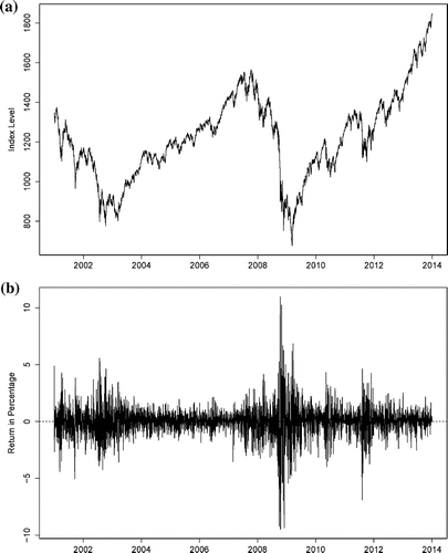
Figure 2. Density plots of S&P 500 return and choices of distributions.

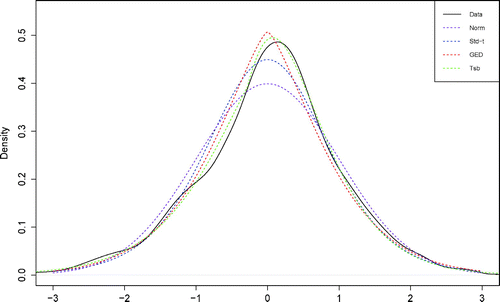
Figure 3. Estimated daily volatility.

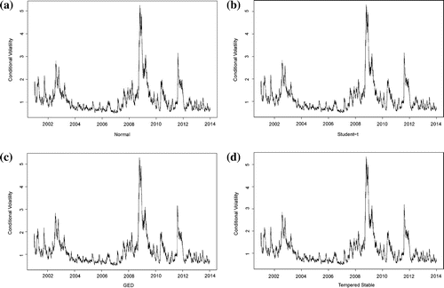
Finally, all the four estimated conditional volatility series⁹ are plotted in Figure 3. Despite their different model performance, the four estimated conditional volatility series demonstrate shapes fairly close to each other. It could be due to the similarity of estimates of GARCH parameters ($\mathit{\omega }$, $\mathit{\alpha }$ and $\mathit{\beta }$). The trends of those series are consistent with our observation of the return series: comparatively more turbulent in the periods 2001–2003 and 2008–2010. This is concordant with the real macro-economic situation: the Dot-com bubble burst at the start of the twenty-first century, and its effect lasted for around two years. On the other hand, the 2008 Global Financial Crisis happened in mid-2008 and last until roughly the end of 2010.

Despite their similarities, the difference between the fitted conditional volatilities can be described as the different in-sample forecasting performance of the fitted models. To quantitatively compare this performance, we measure the prediction error for each model by $\left|\sqrt{{\widehat{h}}_t}-|r_t|\right|$, where ${\widehat{h}}_t$ is the fitted $h_t$ for each model, and $|r_t|$ is employed to proxy the true conditional volatility. The results are reported in Panel A of Table 5. Moreover, to consider the out-of-sample forecasts, we use the last 100 observations as the prediction sample and the others as the training sample. Then, we fit each model for the training sample and calculate the one-step ahead forecast of $h_t$. After that, we include the first observation in the training sample and generate another one-step-ahead forecast. We repeat this rolling-window approach until 100 such one-step-ahead forecasts are produced. Then, we calculate the absolute difference between them and the corresponding $|r_t|$, which measures the out-of-sample forecasting errors. The results are reported in Panel B of Table 5. It is observed that GARCH-S leads to the smallest average forecasting errors in both the in-sample and out-of-sample cases. GARCH-S also generates the smallest variations of forecasting errors, as measured by the standard deviation. Additionally, in terms of the average forecasting errors, GARCH-G outperforms the GARCH-t, and GARCH-N is the least preferred model in both cases.

6. Conclusion

GARCH model has enjoyed particular popularity in the finance research. Despite its well-established properties, in practice, GARCH model can lead to more efficient estimates when an appropriate fat-tailed distribution is employed. As widely used alternatives, the Student’s t-distribution and the GED are the popular choices in many existing studies. However, a recent study by Calzolari et al. (2014) points out that due to the instability under aggregation, the Student’s t and GED are not optimal choices. Motivated by those findings, this paper aims to find an appropriate distribution for disturbances of the GARCH model, when the underlying distribution is a fat-tailed but unknown type.

Calzolari et al. (2014) introduce the $\mathit{\alpha }$-stable distribution, which outperforms the Student’s t and GED for its stability-under-aggregation feature. Unfortunately, the undefined second moment of this candidate brings in even more serious problems. To solve this issue, our paper argues that the tempered stable distribution should be employed instead. Via systematically designed simulation studies on the GARCH process, we systematically demonstrate the appropriateness of the tempered stable distribution applied in the GARCH model. The first two studies assume that the true distributions are the Student’s t and GED, respectively. In such cases, results of GARCH-S are close to those of the true models. Additionally, GARCH-S outperforms the other competing models in terms of consistency, efficiency and overall performance. We construct different combinations of the tempered stable distribution to simulate the GARCH process in the third study. Our results suggest that none of the GARCH-N, GARCH-t and GARCH-G can perform as well as the GARCH-S model.

Finally, empirical evidence is further provided to check the robustness of our simulation results in practice. We fit the daily return of the S&P 500 index into the four GARCH models respectively. Our results indicate that GARCH-S is still preferred to all the other models, and the density of the fitted tempered stable distribution is the closest to the smoothed estimates of the data.

In particular, we demonstrate that GARCH-S has better in- and out-of-sample forecasting performance than all the other models. Hence, the tempered stable distribution could be a widely useful tool for modelling the financial volatility in general contexts with a GARCH-type specification. For instance, financial practitioners can use GARCH-S to significantly increase the accuracy of their risk measures, which can further benefit their portfolio management and other enterprise risk management issues.

Acknowledgements

We are grateful to the ANU College of Business and Economics and Research School of Finance, Actuarial Studies and Statistics and Jiangxi University of Finance and Economics for their support. The authors would also like to thank Dave Allen, Felix Chan, Michael McAleer, Paresh Narayan, Morten Nielson, Albert Tsui, Zhaoyong Zhang, and participants at the 1st Conference on Recent Developments in Financial Econometrics and Applications, the 8th China R Conference (Nanchang), ANU Research School Brown Bag Seminar, Central University of Finance and Economics Seminar, China Meeting of Econometric Society, Chinese Economists Society China Annual Conference, Econometric Society Australasian Meeting, Ewha Woman’s University Department of Economics Seminar, International Congress of the Modelling and Simulation Society of Australia and New Zealand and Shandong University Seminar. We especially thank the editors and two anonymous referees for their helpful comments and suggestions. The usual disclaimer applies.

Additional information

Funding

The authors received no direct funding for this research.

Notes on contributors

Lingbing Feng

Lingbing Feng is an assistant professor of Statistics in the Jiangxi University of Finance and Economics. Highest academic degree: PhD in Statistics, the Australian National University (2015). Research interests: time series analysis; spatial-temporal statistics.

Yanlin Shi

Yanlin Shi is a Senior Lecturer of Actuarial Studies in the Macquarie University. Highest academic degree: PhD in Statistics, the Australian National University (2014). Research interests: time series analysis; applied econometrics; quantitative risk modelling.

Notes

1 In this case, the associated Levy processes are called “truncated Levy flights”, the appropriateness of which to be applied in the GARCH model is also discussed in Constantinides and Savel’ev (2013).

2 Since the mean of ${\mathit{\epsilon }}_t$ is 0, ${\mathit{\eta }}_t$ is sometimes named as standardized residual.

3 As argued by Mittnik, Doganoglu, and Chenyao (1999), compared to other approximation methods, discrete Fourier transform is accurate and efficient to estimate parameters of stable family distributions, especially when $N=2^{13}$ or above. Therefore, we set N as $2^{15}$ in this paper.

4 Different random number generators may have their own algorithms to apply the pseudo values to produce the simulations. We discard the first few replicates to avoid any bias or cycling effects may exist in those algorithms.

5 Since either $\mathit{\alpha }$ or $\mathit{\beta }$ itself cannot be interpreted for financial data, we also report the comparison of volatility persistence indicated by $\mathit{\alpha }+\mathit{\beta }$.

6 Although tempered stable distribution has four more parameters than Student’s t-distribution, the improvement of log-likelihood is still a positive indicator that GARCH-S can lead to satisfied results even when the true distribution is not tempered stable.

7 Standardized residuals are extracted from GARCH(1,1)-N model.

8 Both values are extracted from the corresponding estimates reported in Table 4.

9 We report conditional volatility here as the square root of $h_t$, so that it has the same scale as $r_t$.

References

- Bianchi, M. L., Rachev, S. T., Kim, Y. S., & Fabozzi, F. J. (2010). Tempered stable distributions and processes in finance: numerical analysis. Mathematical and Statistical Methods for Actuarial Sciences and Finance (pp. 33–42). Italy: Springer.
- Bollerslev, T. (1986). Generalized autoregressive conditional heteroskedasticity. Journal of Econometrics, 31, 307–327.
- Bollerslev, T. (1987). A conditional heteroskedastic time series model for speculative prices and rates of return. Review of Economics and Statistics, 69, 542–547.
- Bollerslev, T., & Wooldridge, J. M. (1992). Quasi-maximum likelihood estimation and inference in dynamic models with time-varying covariances. Econometric Reviews, 11, 143–172.
- Calzolari, G., Halbleib, R., & Parrini, A. (2014). Estimating garch-type models with symmetric stable innovations: Indirect inference versus maximum likelihood. Computational Statistics & Data Analysis, 76, 158–171.
- Carr, P., Geman, H., Madan, D. B., & Yor, M. (2002). The fine structure of asset returns: An empirical investigation*. The Journal of Business, 75, 305–333.
- Chkili, W., Aloui, C., & Nguyen, D. K. (2012). Asymmetric effects and long memory in dynamic volatility relationships between stock returns and exchange rates. Journal of International Financial Markets, Institutions and Money, 22, 738–757.
- Constantinides, A., & Savel’ev, S. (2013). Modelling price dynamics: A hybrid truncated lévy flight\^{s}cgarch approach. Physica A, 392, 2072–2078.
- Cont, R., & Tankov, P. (2004). Financial modelling with jump processes. London: Chapman and Hall/CRS Press.
- Engle, R. F. (1982). Autoregressive conditional heteroskedasticity with estimates of variance of united kingdom inflation. Economerica, 50, 987–1007.
- Fan, Y., Zhang, Y.-J., Tsai, H.-T., & Wei, Y.-M. (2008). Estimating ‘value at risk’ of crude oil price and its spillover effect using the ged-garch approach. Energy Economics, 30, 3156–3171.
- Feng, L., & Shi, Y. (2016). Fractionally integrated garch model with tempered stable distribution: A simulation study. Journal of Applied Statistics, 1–21.
- Ho, K.-Y., Shi, Y., & Zhang, Z. (2013). How does news sentiment impact asset volatility? evidence from long memory and regime-switching approaches. North American Journal of Economics and Finance, 26, 436–456.
- Kim, Y. S., Rachev, S. T., Bianchi, M. L., & Fabozzi, F. J. (2008). Financial market models with lévy processes and time-varying volatility. Journal of Banking & Finance, 32, 1363–1378.
- Koponen, I. (1995). Analytic approach to the problem of convergence of truncated lévy flights towards the gaussian stochastic process. Physical Review E, 52, 1197–1199.
- Küchler, U., & Tappe, S. (2013). Tempered stable distributions and processes. Stochastic Processes and their Applications, 123, 4256–4293.
- Mabrouk, S., & Saadi, S. (2012). Parametric value-at-risk analysis: Evidence from stock indices. The Quarterly Review of Economics and Finance, 52, 305–321.
- Mittnik, S., Doganoglu, T., & Chenyao, D. (1999). Computing the probability density function of the stable paretian distribution. Mathematical and Computer Modelling, 29, 235–240.
- Podobnika, B., Horvaticd, D., Petersena, A. M., & Stanleya, H. E. (2009). Cross-correlations between volume change and price change. Proceedings of the National Academy of Sciences of the United States of America, 106, 22079–22084.
- Shi, Y., & Feng, L. (2015). A discussion on the innovation distribution of markov regime-switching garch model. Economic Modelling, 53, 278–288.
- Stanley, H. E., Plerou, V., & Gabaix, X. (2008). A statistical physics view of financial fluctuations: Evidence for scaling and universality. Physica A, 387, 3967–3981.
- Susmel, R., & Engle, R. F. (1994). Hourly volatility spillovers between international equity markets. Journal of International Money and Finance, 13, 3–25.
- Yang, S.-R., & Brorsen, B. W. (1993). Nonlinear dynamics of daily futures prices: conditional heteroskedasticity or chaos? Journal of Futures Markets, 13, 175–191.
- Zhu, D., & Galbraith, J. W. (2011). Modeling and forecasting expected shortfall with the generalized asymmetric student-t and asymmetric exponential power distributions. Journal of Empirical Finance, 18, 765–778.