On skewed, leptokurtic returns and pentanomial lattice option valuation via minimal entropy martingale measure

Abstract

This article develops, a lattice-based approach for pricing contingent claims when parameters governing the logs of the underlying asset dynamics are modelled by generalized hyperbolic distribution and normal inverse Gaussian distribution. The pentanomial lattice is constructed using a moment matching procedure. Moment generating functions of generalized hyperbolic distribution and normal inverse Gaussian distribution are utilized to compute probabilities and jump parameters under historical measure $\mathbb{P}$. Minimal entropy martingale measure (MEMM) is used to value European call option with a view of comparing the results with some of the existing benchmark model such as Black Scholes model. Empirical data from S&P500 index, RUTSELL2000 index and RUI1000 index are used to demonstrate how the model works. There is a significant difference especially for long term maturity (six months and above) type of contracts, the proposed model outperform the benchmark model, while performing poorly at short term contracts. Pentanomial NIG models seems to outperform the other models especially for long dated maturities.

Keywords:

• binomial
• pentanomial lattice
• generalized hyperbolic distribution
• normal inverse Gaussian
• minimal entropy martingale measure
• European call option

Public Interest Statement

This study develops a simplified approach to value financial contracts such as calls and puts. Features of daily relative changes of price are known to be non-normal in contrast to the common assumption. The proposed model accommodates such several aspects of reality observed in financial markets in recent times. Subjected to observed market data, the proposed valuation model seems to outperform existing benchmark models. The simplified approach may be used to value different types of contracts which may not have closed-form solutions.

1. Introduction

In the past decade option pricing has become one of the major areas of financial theory and practice. Since the introduction of the celebrated Black Scholes option pricing which assumes that the underlying stock prices follow a geometric Brownian motion; there is an explosive growth in trading derivatives in the world wide financial market. Due to its compact and computational simplicity; the Black and Scholes (1973) model enjoys great popularity in the financial markets. Recently the formulae has been extended in various ways. Recent studies have shown that the normal distribution may not accurately describe observed properties of stock returns; see for example Barndorff-Nielsen (1998), Cont (2001), Carr, German, Madan, and Yor (2002) for a well documented stylized facts about returns. The deviations from normality become more severe when high frequency financial data are used.

A lattice is a graphical representation of all possible paths that might be followed any stochastic process say for example stock price. We construct a pentanomial lattice that approximates the evolution stock price. Lattices are useful for valuing a wide variety of options such as path dependent contracts which may not have a closed form solution such as lookback options, American type options and barrier option. Since options cash flow are functions of the future value of the underlying asset, options can be valued in the lattice by taking the expectation of their payoff. The current option value equals the discounted expected option payoff.

Lattices for option pricing were first introduced in 1979 in the pioneering work of Cox, Ross, and Rubinstein (1979). In particular, they used binomial lattice to model geometric Brownian motion and Rendleman and Bartter (1979) used binomial lattice to model exponential Poisson process. An attractive property of their model is that the binomial lattice for geometric Brownian motion is consistent with the standard (Black & Scholes, 1973) formula for European options. Due to simplicity and versatility of lattice models, a number of extensions to the basic model have been proposed, see Derman and Kani (1994), Ritchken and Trevor (1999), Yamada and Primbs (2001), Wu (2006) for example. Florescu and Viens (2008) use quadrinomial tree to model stochastic volatility in option pricing, while Primbs, Rathianam, and Yamada (2007) price options with a pentanomial lattice. It is worthy noting that an efficient lattice method, may be significantly faster than a Monte Carlo method for valuing some types of path dependent options.

The objective of this paper is to develop an option pricing lattice model which combine skewness and the leptokurtic nature of daily log returns under an alternative distributional assumption, that is consistent with empirical stock returns. Minimal entropy martingale measure (MEMM) is used to change probability measure $\mathbb{P}$ to a risk neutral economy within a pentanomial lattice framework. Parameters of the model are selected to match the first four central moments of the returns. Such a model, has the potential of estimating option prices that are more consistent with empirically observed stylized facts of returns.

This paper proceeds as follows. In Section 2, we establish the general dynamics of the asset price over a time interval $\mathrm{\Delta }\mathit{\tau }$. In Section 3, a brief review of binomial, and pentanomial lattice is outlined. In Section 4, option pricing formulaes are derived in pentanomial framework and minimal entropy martingale measure is applied to change measure $\mathbb{P}$ to risk neutral world $\mathbb{Q}.$ Section 4 introduces numerical procedures in relation to derived formulaes using real market data. European call option is priced and numerical results compared. Section draws conclusions.

2. Basic model setup

Consider the stochastic distribution of the price of non-divided paying stock in a risk-neutral economy. Let the stock price be S(t) at time t in a period $[t,T]$. An option pricing model is generally based on assumed process of the stock price or return. The Black and Scholes (1973), for example assume that the stock price (under risk neutral measure $\mathbb{Q}$), movement is governed by the following process$$\begin{array}{c}\hfill \text{d}S(t)=rS(t)\text{d}t+\mathit{\sigma }S(t)\text{d}{B}_t,\Rightarrow S_T|{\mathcal{F}}_t=S_{t}exp\left(\left(r-\frac{{\mathit{\sigma }}^2}{2}\right)(T-t)+\mathit{\sigma }\sqrt{T-t}{Z}_t\right),Z_t\sim N(0,1)\end{array}$$

where r is the risk free rate and $\mathit{\sigma }$ is the instantaneous volatility rate of the stock return distribution. This is equivalent to assuming daily log returns are normally distributed with mean $(r-{\mathit{\sigma }}^2/2)(T-t)$ and variance ${\mathit{\sigma }}^2(T-t)$. The resulting price of a contingent claim $max(S_T-K,0)$ is given by(2.1) $$\begin{array}{cc}\hfill C^{BS}(t,K)& =S_t\mathrm{\Phi }(d_1)-K{e}^{-r(T-t)}\mathrm{\Phi }(d_2)\hfill \\ \hfill d_1& =\frac{ln(S_t/K{e}^{r(T-t)})}{\mathit{\sigma }\sqrt{T-t}}+\frac{1}{2}\mathit{\sigma }\sqrt{T-t}\hfill \\ \hfill d_2& =\frac{ln(S_t/K{e}^{r(T-t)})}{\mathit{\sigma }\sqrt{T-t}}-\frac{1}{2}\mathit{\sigma }\sqrt{T-t}\hfill \end{array}$$(2.1)

where t refers to the current time. However such a process does not incorporate skewness and leptokurtic fat tails which are typically associated with empirical stock log returns.

We consider a discrete time economy for a period of [t, T] where the trading takes place at any of the $n+1$ trading nodes $t,t+\mathrm{\Delta }\mathit{\tau },t+2\mathrm{\Delta }\mathit{\tau },\dots ,t+n\mathrm{\Delta }\mathit{\tau }$ where $\mathrm{\Delta }\mathit{\tau }=\frac{T-t}{n}$. Suppose $(\mathrm{\Omega },\mathbb{F},\mathbb{P})$ is a given probability space, where $\mathbb{P}$ is the statistical or data generating probability measure. Here, the sample space $\mathbb{F}$ represents the uncertainty in our financial model. Let $\mathfrak{T}$ be the time index set $\{t,t+\mathrm{\Delta }\mathit{\tau },t+2\mathrm{\Delta }\mathit{\tau },\dots ,t+n\mathrm{\Delta }\mathit{\tau }\}$ of our financial model such that all economic activities take place at each time point $t\in \mathfrak{T}.$ We equip our probability space $(\mathrm{\Omega },\mathbb{F},\mathbb{P})$ with the information structure $\mathcal{F}:={\{{\mathcal{F}}_j\}}_{j\in \mathfrak{T}}$ to get a filtered probability space denoted by $(\mathrm{\Omega },\mathbb{F},{({\mathcal{F}}_t)}_{t\in [0,T]},\mathbb{P})$. That is, for each $j\in \mathfrak{T},{\mathcal{F}}_j$ represents the information set of all market information up to and including time j,  where ${\mathcal{F}}_0$ contains all $\mathbb{P}$-null sets in $\mathbb{F}.$ In general, asset price $S_{i\mathrm{\Delta }\mathit{\tau }}$ is sometimes assumed to follow the process(2.2) $$\begin{array}{c}\hfill \frac{S_{i\mathrm{\Delta }\mathit{\tau }}}{S_{(i-1)\mathrm{\Delta }\mathit{\tau }}}=exp\left(\mathit{\mu }+\sum _{k=1}^d{\mathit{\varphi }}_{k}ln\left(\frac{S_{(i-k)\mathrm{\Delta }t}}{S_{(i-k-1)\mathrm{\Delta }t}}\right)+{\mathit{\sigma }}_{i\mathrm{\Delta }t}\left[Z_i+\sum _{j=1}^{N_i(\mathrm{\Delta }t)}{W}_i^{(j)}(\mathrm{\Delta }t)\right]\right)\end{array}$$(2.2)

where $Z_i\sim N(0,1)$, $W_i^{(j)}(\mathrm{\Delta }\mathit{\tau })\sim N(\mathit{\mu }(\mathrm{\Delta }\mathit{\tau }),{\mathit{\gamma }}^2(\mathrm{\Delta }\mathit{\tau }))$, and $N_i(\mathrm{\Delta }t),i=1,2,\dots ,n$ are sequences of independent Poisson random variables with parameter $\mathit{\lambda }\mathrm{\Delta }\mathit{\tau }$. Changes of daily log returns are known to be leptokurtic and assumed to be laced with Poisson mixture of normal distributions. For more detailed exposition on modeling the dynamics of the underlying risky asset see Hsieh (1989), Nieuwland, Verschoor, and Wolff (1994), Chan and Maheu (2002), Duan, Ritchken, and Sun (2006) etc. Without loss of generality, our focus is on developing lattice model for the underlying process, say(2.3) $$\begin{array}{c}\hfill S_T|{\mathcal{F}}_t=S_{t}exp(m_t+X_t).\end{array}$$(2.3)

where $m_t$ is a well chosen constant. Let $Y_t=m_t+X_t$, and define $Y_i:=log(S_{i\mathrm{\Delta }\mathit{\tau }}/S_{(i-1)\mathrm{\Delta }\mathit{\tau }}),i=1,\dots ,n$, which are assumed to be random variable whose first four moments are known from the market data simply for the sake of developing a pentanomial lattice framework. For simplicity, we let $Y_t$ be modelled by generalized hyperbolic distribution and normal inverse Gaussian which are as defined below.

2.1. The generalized hyperbolic distribution

In this subsection we provide definition of the generalized hyperbolic distribution along with normal inverse Gaussian as its special case.

Definition 2.1

The probability density function of the one-dimensional Generalized Hyperbolic distribution is given by the following:(2.4) $$\begin{array}{c}\hfill f_{GH}(y;\mathit{\alpha },\mathit{\beta },\mathit{\delta },\mathit{\mu },\mathit{\lambda })=\frac{{(\mathit{\gamma }/\mathit{\delta })}^{\mathit{\lambda }}}{\sqrt{2\mathit{\pi }}{K}_{\mathit{\lambda }}(\mathit{\delta }\mathit{\gamma })}·\frac{K_{\mathit{\lambda }-\frac{1}{2}}(\mathit{\alpha }\sqrt{{\mathit{\delta }}^2+{(y-\mathit{\mu })}^2})}{{(\sqrt{{\mathit{\delta }}^2+{(y-\mathit{\mu })}^2}/\mathit{\alpha })}^{\frac{1}{2}-\mathit{\lambda }}}·e^{\mathit{\beta }(y-\mathit{\mu })}\end{array}$$(2.4)

where ${\mathit{\gamma }}^2={\mathit{\alpha }}^2-{\mathit{\beta }}^2$ and $K_{\mathit{\lambda }}$ is the modified Bessel function of third kind with index $\mathit{\lambda }$ given by(2.5) $$\begin{array}{c}\hfill K_{\mathit{\lambda }}(\mathit{\omega })=\frac{1}{2}\underset{0}{\overset{\infty }{\int }}exp\left[-\frac{\mathit{\omega }}{2}(v^{-1}+v)\right]v^{\mathit{\lambda }-1}dv\end{array}$$(2.5) .

According to Barndorff-Nielsen, the parameters domain is given by$$\begin{array}{cc}& \mathit{\alpha }>0{\mathit{\alpha }}^2>{\mathit{\beta }}^2\mathit{\delta }\ge 0\text{for}\mathit{\lambda }>0,\hfill \\ \hfill & \mathit{\alpha }>0{\mathit{\alpha }}^2>{\mathit{\beta }}^2\mathit{\delta }>0\text{for}\mathit{\lambda }=0,\hfill \\ \hfill & \mathit{\alpha }>0{\mathit{\alpha }}^2\ge {\mathit{\beta }}^2\mathit{\delta }>0\text{for}\mathit{\lambda }<0.\hfill \end{array}$$

In all cases, $\mathit{\mu }$ is the location parameter and can take any real value, $\mathit{\delta }$ is a scale parameter; $\mathit{\alpha }$ and $\mathit{\beta }$ determine the distribution shape and $\mathit{\lambda }$ defines the subclasses of GH and is related to the tail flatness.

Characteristic function of the GH is given by(2.6) $$\begin{array}{c}\hfill {\mathit{\phi }}_{GH}(u)=e^{iu\mathit{\mu }}{\left(\frac{{\mathit{\alpha }}^2-{\mathit{\beta }}^2}{{\mathit{\alpha }}^2-{(\mathit{\beta }+iu)}^2}\right)}^{\mathit{\lambda }/2}\frac{K_{\mathit{\lambda }}\left(\mathit{\delta }\sqrt{{\mathit{\alpha }}^2-{(\mathit{\beta }+iu)}^2}\right)}{K_{\mathit{\lambda }}\left(\mathit{\delta }\sqrt{{\mathit{\alpha }}^2-{\mathit{\beta }}^2}\right)},\end{array}$$(2.6)

while mean and variance are given respectively by the following$$\begin{array}{cc}\hfill \mathbb{E}(Y)& =\mathit{\mu }+\frac{\mathit{\beta }\mathit{\delta }}{\sqrt{{\mathit{\alpha }}^2-{\mathit{\beta }}^2}}\frac{K_{\mathit{\lambda }+1}(\mathit{\zeta })}{K_{\mathit{\lambda }}(\mathit{\zeta })}\hfill \\ \hfill \mathbb{V}(Y)& ={\mathit{\delta }}^2\left(\frac{K_{\mathit{\lambda }+1}(\mathit{\zeta })}{\mathit{\zeta }{K}_{\mathit{\lambda }}(\mathit{\zeta })}+\frac{{\mathit{\beta }}^2}{{\mathit{\alpha }}^2-{\mathit{\beta }}^2}\left[\frac{K_{\mathit{\lambda }+2}(\mathit{\zeta })}{K_{\mathit{\lambda }}(\mathit{\zeta })}-{\left(\frac{K_{\mathit{\lambda }+1}(\mathit{\zeta })}{K_{\mathit{\lambda }}(\mathit{\zeta })}\right)}^2\right]\right),\text{where}\mathit{\zeta }=\mathit{\delta }\sqrt{{\mathit{\alpha }}^2-{\mathit{\beta }}^2}\hfill \end{array}$$

We consider normal inverse Gaussian (hereafter NIG) which is a special case of Generalized hyperbolic distributions when $\mathit{\lambda }=-0.5$.

Definition 2.2

The Normal inverse Gaussian (hereafer NIG) distribution is a flexible four parameter distribution that can describe a wide range of shapes. A random variable $Y\sim NIG(\mathit{\alpha },\mathit{\beta },\mathit{\delta },\mathit{\mu })$ if(2.7) $$\begin{array}{c}\hfill f_{\text{NIG}}(y;\mathit{\alpha },\mathit{\beta },\mathit{\delta },\mathit{\mu })=\frac{\mathit{\alpha }}{\mathit{\pi }}exp\left(\mathit{\delta }\left[\sqrt{{\mathit{\alpha }}^2-{\mathit{\beta }}^2}+\mathit{\beta }\mathit{\zeta }(y)\right]\right)\frac{K_1(\mathit{\alpha }\mathit{\delta }\sqrt{1+\mathit{\zeta }{(y)}^2})}{\sqrt{1+\mathit{\zeta }{(y)}^2}},\mathit{\zeta }(y)=\frac{(y-\mathit{\mu })}{\mathit{\delta }}\end{array}$$(2.7)

where $K_1$ is the modified Bessel function of third kind, with the index 1 given by$$\begin{array}{c}\hfill K_1(\mathit{\omega })=\frac{1}{2}\underset{0}{\overset{\infty }{\int }}exp\left[-\frac{\mathit{\omega }}{2}(v^{-1}+v)\right]dv\end{array}$$

It is interesting to note that NIG distribution can take a variety of different shapes. Having a heavier tail than that of normal distribution is considered suitable for modeling data sets with many extremal observations. The moments of a random variable $Y\sim NIG(\mathit{\alpha },\mathit{\beta },\mathit{\mu },\mathit{\delta })$ are(2.8) $$\begin{array}{c}\hfill \mathbb{E}[Y]=\mathit{\mu }+\mathit{\delta }\frac{\mathit{\beta }}{\mathit{\gamma }},\mathbb{V}[Y]=\mathit{\delta }\frac{{\mathit{\alpha }}^2}{{\mathit{\gamma }}^3},\text{where}\mathit{\gamma }=\sqrt{{\mathit{\alpha }}^2-{\mathit{\beta }}^2}\\ \hfill \end{array}$$(2.8)

The characteristic function of NIG random variable say Y is given by(2.9) $$\begin{array}{c}\hfill {\mathit{\phi }}_{\text{NIG}}(u)=\mathbb{E}[exp(iuy)]=exp(i\mathit{\mu }u)\frac{exp(\mathit{\delta }\sqrt{{\mathit{\alpha }}^2-{\mathit{\beta }}^2})}{exp(\mathit{\delta }\sqrt{{\mathit{\alpha }}^2-{(\mathit{\beta }+iu)}^2})}\end{array}$$(2.9)

2.2. Parameterizations

Although the parametrization $(\mathit{\alpha },\mathit{\beta },\mathit{\delta },\mathit{\mu },\mathit{\lambda })$ is mostly used in literature we have other parameterizations like $(\mathit{\chi },\mathit{\xi },\mathit{\delta },\mathit{\mu })$ which is invariant under the transformation of the scale and location parameters with $\mathit{\xi }={(1+\mathit{\delta }\sqrt{{\mathit{\alpha }}^2-{\mathit{\beta }}^2})}^{-1/2}$ and $\mathit{\chi }=\mathit{\xi }\mathit{\beta }/\mathit{\alpha }$. McNeil, Frey, and Embrechts (2005) used the following parameterizations $(\mathit{\lambda },\mathit{\chi },\mathit{\psi },\mathit{\mu },\mathit{\sigma },\mathit{\gamma })$ where(2.10) $$\begin{array}{c}\hfill \mathit{\lambda }=\mathit{\lambda },\mathit{\beta }=\frac{\mathit{\gamma }}{{\mathit{\sigma }}^2},\mathit{\delta }=\mathit{\sigma }\sqrt{\mathit{\chi }},\mathit{\alpha }=\sqrt{\frac{\mathit{\psi }}{{\mathit{\sigma }}^2}+{\mathit{\beta }}^2}\end{array}$$(2.10)

The parametrization $(\mathit{\lambda },\overline{\mathit{\alpha }},\mathit{\mu },\mathit{\sigma },\mathit{\gamma })$, is derived if we set$$\begin{array}{c}\hfill \overline{\mathit{\alpha }}=\sqrt{\mathit{\psi }\mathit{\chi }},\text{and}\sqrt{\frac{\mathit{\chi }}{\mathit{\psi }}}\frac{K_{\mathit{\lambda }+1}(\sqrt{\mathit{\psi }\mathit{\chi }})}{K_{\mathit{\lambda }}(\sqrt{\mathit{\psi }\mathit{\chi }})}=1,\text{which implies},\mathit{\psi }=\overline{\mathit{\alpha }}\frac{K_{\mathit{\lambda }+1}(\overline{\mathit{\alpha }})}{K_{\mathit{\lambda }}(\overline{\mathit{\alpha }})},\mathit{\chi }=\overline{\mathit{\alpha }}\frac{K_{\mathit{\lambda }}(\overline{\mathit{\alpha }})}{K_{\mathit{\lambda }+1}(\overline{\mathit{\alpha }})}.\end{array}$$

Similar parametrization is used in ghyp R package.

The main challenge is to construct branching probabilities in the lattice. Our approach would be using moment matching technique.

3. Multinomial lattices

One of the most important joint distributions is the multinomial distribution, which arises when a sequence of n independent and identical experiments are performed. Suppose that each experiment can result in any one of $\mathcal{L}$ possible outcomes, with respective probabilities $p_1,p_2,\dots ,p_{\mathcal{L}},{\sum }_{j=1}^{\mathcal{L}}{p}_j=1$. If we let $X_i$ denote the number of the n experiments that result in outcome number i, then(3.1) $$\begin{array}{c}\hfill \mathbb{P}(X_1=n_1,X_2=n_2,\dots ,X_{\mathcal{L}}=n_{\mathcal{L}})=\frac{n!}{n_1!n_2!\dots n_{\mathcal{L}}!}{p}_1^{n_1}{p}_2^{n_2}\dots p_{\mathcal{L}}^{n_{\mathcal{L}}},\sum _{j=1}^{\mathcal{L}}{n}_j=n.\end{array}$$(3.1)

In multinomial lattice model, we need to determine the up and down rates u and d, and the probabilities $p_1,\dots ,p_{\mathcal{L}}$ to fit the actual market data as closely as possible. This can be done by moment matching or directly from density function, see Kellezi and Webber (2004) for different ways of constructing branching probabilities in the lattice. Note that u and d may be thought of as up and down factors at each step. Also it can be shown that the multinomial lattice still recombines even if u and d are time dependent when $u_n/d_n=c$ is satisfied for some constant $c>1$ where $u_n$ and $d_n$$n=0,1,\dots ,N-1$ are up and down factors in each time step, see Yamada and Primbs (2001), Yamada and Primbs (2004) for more details. Let the up and down rates, u and d, be given as(3.2) $$\begin{array}{c}\hfill u:=exp\left(\frac{m_t}{\mathcal{L}-1}+\mathit{\alpha }\right),d:=exp\left(\frac{m_t}{\mathcal{L}-1}-\mathit{\alpha }\right)\end{array}$$(3.2)

where $\mathcal{L}$ is the number of branches, and $m_t=\mathbb{E}[Y_t]$ and $\mathit{\alpha }>0$ are real numbers.

We develop the basic theoretical set up to model the dynamics of the underlying with an objective to value options in discrete time. It is assumed that, trades occur only at discrete dates indexed by $\{0<\mathrm{\Delta }\mathit{\tau },\dots ,<n\mathrm{\Delta }\mathit{\tau }\}$, and the stock price at date $t+i\mathrm{\Delta }\mathit{\tau }$ can take on values only in a discrete set specified exogenously by$$\begin{array}{c}\hfill {\tilde{S}}_{(t+k\mathrm{\Delta }\mathit{\tau },j)},j=1,\dots ,(\mathcal{L}-1)k+1,k=0,\dots ,n\end{array}$$

where the variables $(t+k\mathrm{\Delta }\mathit{\tau },j)$, index time and state values respectively, while $\mathcal{L}$ is the possible number of future states for ${\tilde{S}}_{t+(k+1)\mathrm{\Delta }\mathit{\tau }}$ from ${\tilde{S}}_{t+k\mathrm{\Delta }\mathit{\tau }}$, i.e.(3.3) $$\begin{array}{c}\hfill {\tilde{S}}_{(t+(k+1)\mathrm{\Delta }\mathit{\tau },l)}=u^{\mathcal{L}-l}{d}^{l-1}{\tilde{S}}_{t+k\mathrm{\Delta }\mathit{\tau }},l=1,\dots ,\mathcal{L}.\end{array}$$(3.3)

with probabilities $p_l,l=1,\dots ,\mathcal{L}$, satisfying $p_1+\cdots +p_{\mathcal{L}}=1$. In this case, the stock may achieve $k(\mathcal{L}-1)+1$ possible prices at time $t=k\mathrm{\Delta }\mathit{\tau },k=0,\dots ,n$ given by(3.4) $$\begin{array}{c}\hfill {\tilde{S}}_{(t+k\mathrm{\Delta }\mathit{\tau },k)}=u^{k(\mathcal{L}-1)+1-k}{d}^{k-1}{S}_t,k=1,\dots ,n(\mathcal{L}-1)+1\end{array}$$(3.4)

Let $Y_k=log(S_{t+k\mathrm{\Delta }\mathit{\tau }}/S_{t+(k-1)\mathrm{\Delta }\mathit{\tau }})$, then its jth central moment,$$\begin{array}{cc}\hfill {\mathit{\mu }}_j& =\mathbb{E}\left[{(Y_k-\mathbb{E}{Y}_k)}^j\right]\hfill \\ \hfill & ={\mathit{\alpha }}^j\sum _{l=1}^{\mathcal{L}}{p}_l{(\mathcal{L}-2l+1)}^j,j\ge 2.\hfill \end{array}$$

For more information about multinomial approximating models see Kamrad and Ritchken (1991), Kargin (2005). We briefly illustrate moment matching methodology, by considering the binomial and pentanomial models for a two time steps in the following subsection.

3.1. Binomial lattices

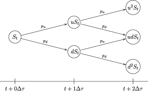
The binomial option pricing model is an iterative solution that models the price evolution over the whole option validity period $[t,T]$. Figure 1 represents the price evolution of the underlying asset as the binomial lattices of all possible prices at equally spaced time steps from today ($t+0\mathrm{\Delta }t$) under the assumption that at each step, the price can move, either up or down at a fixed rate and with respective pseudo-probabilities $p_u$ and $p_d$. A standard (Cox et al., 1979) binomial tree, consists of a set of nodes, representing possible future stock prices, with a constant logarithmic spacing between these nodes.

Figure 1. Binomial lattice in two time steps.

The necessary equations for the binomial lattice are $p_u+p_d=1,$(3.5) $$\begin{array}{cc}\hfill \sum _{l=1}^2{p}_l(\mathcal{L}-2l+1)& =p_1-p_2=0,\mathcal{L}=2.\hfill \end{array}$$(3.5)

From these two equations, we obtain several possibilities of solutions e.g. $p_u=p_d=\frac{1}{2}.$ or$$\begin{array}{c}\hfill p_u=\frac{1}{2}+\frac{1}{2}\frac{\mathit{\mu }}{\mathit{\sigma }}\sqrt{\mathrm{\Delta }\mathit{\tau }},p_d=\frac{1}{2}-\frac{1}{2}\frac{\mathit{\mu }}{\mathit{\sigma }}\sqrt{\mathrm{\Delta }\mathit{\tau }}\text{with}u=e^{\mathbb{E}{Y}_i+\mathit{\sigma }}\text{and}d=e^{\mathbb{E}{Y}_i-\mathit{\sigma }},\end{array}$$

where $\mathit{\sigma }$ is the variance of Y. A European call option with exercise price K and date n will have payoff in state $[n,j]$ given by(3.6) $$\begin{array}{c}\hfill C(n,j)=\sum _{j=0}^n{q}_1^j{(1-q_1)}^{j-n}\frac{n!}{j!(n-j)!}max[S_t{u}^j{d}^{n-j}-K,0],q_1=1-q_2\in \mathbb{Q}\end{array}$$(3.6)

3.2. Pentanomial lattice construction

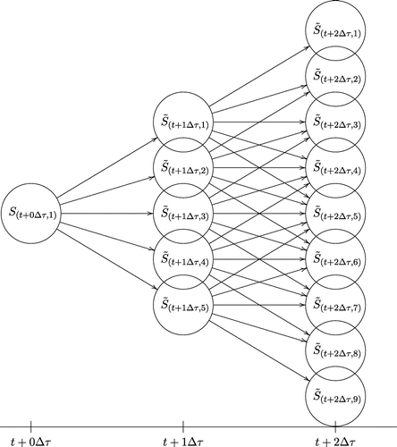
We consider state space for risky stock price dynamics over two trading dates as shown in Figure 2. At each date $k\mathrm{\Delta }\mathit{\tau }$, the stock price can take on values in an exogenously specified discrete set indexed by j. The price $\tilde{S}(t+k\mathrm{\Delta }\mathit{\tau },j)$ denotes the stock price in state j at date $k\mathrm{\Delta }\mathit{\tau }$ for $k=1,...,N$ and $j=1,\dots ,4k+1$ respectively.

Figure 2. Pentanomial lattice for risky stock price dynamics over two trading dates.

To construct a pentanomial model of stock prices, we examine the behavior of the stock price in an interval $[t,t+\mathrm{\Delta }\mathit{\tau }]$. The discrete distribution of $Y_i$ over the interval $[t,t+i\mathrm{\Delta }\mathit{\tau }]$ is approximated to be pentanomial,as illustrated in Figure 2. To model the stock price movement as a pentanomial lattice, the interval [t, T] is divided into n equal subintervals of length $\mathrm{\Delta }\mathit{\tau }=(T-t)/n$, where T is the maturity date of an option. For convenience, define $S_T^{\ast }=S_T/S_t$. To develop an option pricing model dependent on skewness and kurtosis, the distribution of $S_T^{\ast }$ is assumed to be fully specified by parameters via central moments.

Proposition 3.1

Let $M_j(T)=\mathbb{E}{[S_T^{\ast }|{\mathcal{F}}_t]}^j={\mathit{\phi }}_Y(-iuj),i=\sqrt{-1}$, and ${\mathit{\mu }}_j(T)=\mathbb{E}{[S_T^{\ast }-M_1(T)]}^j,j=1,2,3,4$ where ${\mathit{\phi }}_Y$ is the characteristic function of random variable Y, and ${\mathit{\mu }}_j(T)$ is the central moment of $S^{\ast }(T).$ Thus$$\begin{array}{cc}\hfill {\mathit{\mu }}_2(T)& =M_2(T)-M_1^2(T)\hfill \\ \hfill {\mathit{\mu }}_3(T)& =M_3(T)-3M_2(T)M_1(T)+2M_1^3(T)\hfill \\ \hfill {\mathit{\mu }}_4(T)& =M_4(T)-4M_3(T)M_1(T)+6M_1^2(T)(M_2^2(T)-3M_1^4(T))\hfill \end{array}$$

It follows that skewness and kurtosis of $S_T^{\ast }$ is given by(3.7) $$\begin{array}{c}\hfill \mathbb{S}(S_T^{\ast }|{\mathcal{F}}_t)=\frac{{\mathit{\mu }}_3(T)}{\mathbb{V}{(S_T^{\ast })}^{3/2}},\mathbb{K}(S_T^{\ast }|{\mathcal{F}}_t)=\frac{{\mathit{\mu }}_4(T)}{\mathbb{V}{(S_T^{\ast })}^2}.\end{array}$$(3.7)

The relation (3.8) is used to form system of linear equations.(3.8) $$\begin{array}{c}\hfill \sum _{l=1}^5{\left([2l-6]\mathit{\alpha }\right)}^k{p}_l={\mathit{\mu }}_k(T),k=1,2,3,4\end{array}$$(3.8)

where ${\mathit{\mu }}_k(T)$ are as defined above.

To calibrate the pentanomial lattice, we need to solve the following five equations(3.9) $$\begin{array}{c}\hfill \begin{array}{c}{p}_1+p_2+p_3+p_4+p_5=1,\hfill \\ -2p_1-p_2+p_4+2p_5=0,\hfill \\ 16p_1+4p_2+4p_4+16p_5=\mathbb{V}(S_T^{\ast })/{\mathit{\alpha }}^2,\hfill \\ -64p_1-8p_2+8p_4+64p_5=\mathbb{S}(S_T^{\ast })\mathbb{V}{(S_T^{\ast })}^{3/2}/{\mathit{\alpha }}^3,\hfill \\ 256p_1+16p_2+16p_4+256p_5=\mathbb{K}(S_T^{\ast })\mathbb{V}{(S_T^{\ast })}^2/{\mathit{\alpha }}^4,\hfill \end{array}\end{array}$$(3.9)

which implies that,(3.10) $$\begin{array}{c}\hfill \left[\begin{array}{ccccc}1& 1& 1& 1& 1\\ -2& -1& 0& 1& 2\\ 16& 4& 0& 4& 16\\ -64& -8& 0& 8& 64\\ 256& 16& 0& 16& 256\end{array}\right]\left[\begin{array}{c}{p}_1\\ p_2\\ p_3\\ p_4\\ p_5\end{array}\right]=\left[\begin{array}{c}1\\ 0\\ \frac{{\mathit{\mu }}_2(T)}{{\mathit{\alpha }}^2}\\ \frac{{\mathit{\mu }}_3(T)}{{\mathit{\alpha }}^3}\\ \frac{{\mathit{\mu }}_4(T)}{{\mathit{\alpha }}^4}\end{array}\right]\end{array}$$(3.10)

Making the column of the probabilities $p_j,j=1,2,3,4,5$ the subject, we get(3.11) $$\begin{array}{c}\hfill \left[\begin{array}{c}{p}_1\\ p_2\\ p_3\\ p_4\\ p_5\end{array}\right]=\frac{1}{384}\left[\begin{array}{ccccc}0& 32& -4& -4& 1\\ 0& -256& 64& 8& -4\\ 384& 0& -120& 0& 6\\ 0& 256& 64& -8& -4\\ 0& -32& -4& 4& 1\end{array}\right]\left[\begin{array}{c}1\\ 0\\ \frac{\mathbb{V}(S_T^{\ast })}{{\mathit{\alpha }}^2}\\ \frac{{\mathit{\mu }}_3(T)}{{\mathit{\alpha }}^3}\\ \frac{{\mathit{\mu }}_4(T)}{{\mathit{\alpha }}^4}\end{array}\right].\end{array}$$(3.11)

The third and fourth equations arise from matching the third and fourth central moments of the approximating distribution to the third and fourth central moments respectively of the empirical distribution. How these central moments are related to skewness and excess kurtosis is described in Equation (3.8). On solving these five equations, we get Equation (3.12),(3.12) $$\begin{array}{c}\hfill \left[\begin{array}{c}{p}_1\hfill \\ p_2\hfill \\ p_3\hfill \\ p_4\hfill \\ p_5\hfill \end{array}\right]=\frac{1}{384}\left[\begin{array}{c}-4A-4B+C\hfill \\ 64A+8B-4C\hfill \\ 384-120A+6C\hfill \\ 64A-8B-4C\hfill \\ -4A+4B+C\hfill \end{array}\right]=\frac{1}{24}\left[\begin{array}{c}\hfill -a-2b+c\\ \hfill 16a+4b-4c\\ \hfill 24-30a+6c\\ \hfill 16a-4b-4c\\ \hfill -a+2b+c\end{array}\right]\end{array}$$(3.12)

where(3.13) $$\begin{array}{c}\hfill A={\mathit{\mu }}_2(T)/{\mathit{\alpha }}^2,B={\mathit{\mu }}_3(T)/{\mathit{\alpha }}^3,C={\mathit{\mu }}_4(T)/{\mathit{\alpha }}^4,a=A/4,b=B/8,c=C/16.\end{array}$$(3.13)

Note that $\mathit{\alpha }$ must be chosen in order to ensure positivity of probabilities $p_1,p_2,p_3,p_4$ and $p_5.$ It so happens that if $\mathbb{K}(S_T^{\ast })\ge 3{\mathbb{S}(S_T^{\ast })}^2-3$ and $\mathbb{K}(S_T^{\ast })\ge \frac{-23}{16}$ then, there exists a range of values of $\mathit{\alpha }$ (which includes $\mathit{\alpha }=\sqrt{\frac{\mathbb{K}(S_T^{\ast })}{12}}$ ) which will ensure that all the probabilities are strictly positive (see Primbs et al., 2007; Yamada & Primbs, 2001; Yamada & Primbs, 2004). This translates to the following proposition.

Proposition 3.2

For the choice of $\mathit{\alpha }=\sqrt{\frac{\mathbb{K}(S_T^{\ast })}{12}}$, Equation (3.12) reduces to the following probabilities in (3.14) with guaranteed positivity, and the corresponding jump amplitudes for the pentanomial lattice in Equation (3.2) respectively.(3.14) $$\begin{array}{cc}& \left[\begin{array}{c}{p}_1\hfill \\ p_2\hfill \\ p_3\hfill \\ p_4\hfill \\ p_5\hfill \end{array}\right]=\frac{1}{4(\mathbb{K}{(S_T^{\ast })}^2)}\left[\begin{array}{c}\hfill 1(\mathbb{K}(S_T^{\ast })-\mathbb{S}(S_T^{\ast })\sqrt{3\mathbb{K}(S_T^{\ast })})\\ \hfill 2(\mathbb{K}(S_T^{\ast })+\mathbb{S}(S_T^{\ast })\sqrt{3\mathbb{K}(S_T^{\ast })})\\ \hfill 2(2\mathbb{K}(S_T^{\ast })-3)\mathbb{K}(S_T^{\ast })\\ \hfill 2(\mathbb{K}(S_T^{\ast })-\mathbb{S}(S_T^{\ast })\sqrt{3\mathbb{K}(S_T^{\ast })})\\ \hfill 1(\mathbb{K}(S_T^{\ast })+\mathbb{S}(S_T^{\ast })\sqrt{3\mathbb{K}(S_T^{\ast })})\end{array}\right]\hfill \end{array}$$(3.14) (3.15) $$\begin{array}{cc}& \left[\begin{array}{c}{a}_1\hfill \\ a_2\hfill \\ a_3\hfill \\ a_4\hfill \\ a_5\hfill \end{array}\right]=\left\{\begin{array}{cc}exp\left(m_t-4\sqrt{\frac{\mathbb{K}(S_T^{\ast })\mathbb{V}(S_T^{\ast })}{12}}\right),\hfill & \text{with probability}{p}_1;\hfill \\ exp\left(m_t-2\sqrt{\frac{\mathbb{K}(S_T^{\ast })\mathbb{V}(S_T^{\ast })}{12}}\right),\hfill & \text{with probability}{p}_2;\hfill \\ exp\left(m_t\right),\hfill & \text{with probability}{p}_3;\hfill \\ exp\left(m_t+2\sqrt{\frac{\mathbb{K}(S_T^{\ast })\mathbb{V}(S_T^{\ast })}{12}}\right),\hfill & \text{with probability}{p}_4;\hfill \\ exp\left(m_t+4\sqrt{\frac{\mathbb{K}(S_T^{\ast })\mathbb{V}(S_T^{\ast })}{12}}\right),\hfill & \text{with probability}{p}_5.\hfill \end{array}\right.\hfill \end{array}$$(3.15)

The notion of change of measure from $\mathbb{P}$ to $\mathbb{Q}$ in an incomplete market implies existence of an equivalent measure which is not unique, with absence of arbitrage. One such martingale measure is minimal entropy martingale measure.

3.3. Minimal entropy martingale measure

One of the most important economic insight underlying the preference free option pricing result, is the concept of perfect replication of contingent claims, by continuously adjusting a self-financing portfolio under the no-arbitrage principle. Cox et al. (1979) provided further insight in the concept of perfect replication by introducing the notion of risk-neutral valuation and establishing its relationship with no-arbitrage principle in a transparent way under a discrete-time binomial setting.

Harrison and Kreps (1979) and Harrison and Pliska (1981) established a solid mathematical foundation for the relationship between no-arbitrage principal and the notion of risk-neutral valuation using the modern language of probability theory. They proposed the “Fundamental theorem for asset pricing” which states that the absence of arbitrage opportunities is equivalent to the existence of an equivalent martingale measure. If the securities market is complete, there is a unique martingale measure and hence the unique price of any contingent claim is given by its discounted payoff at expiry under the martingale measure. However, the assumption of market completeness is questionable in the real world securities market. Under an incomplete market, there is more than one equivalent martingale measure and hence a range of no-arbitrage prices for a contingent claim. One crucial issue is to identify an equivalent martingale measure which gives an economically consistent and justifiable price for the contingent claim.

Let $n=5$ be the cardinality of $\mathrm{\Omega }$, $R=1+r$ (where r denotes single period interest rate) and $S=(S_{t+0\mathrm{\Delta }\mathit{\tau }},{\tilde{S}}_{t+1\mathrm{\Delta }\mathit{\tau }})$ be the price process of the risky asset. We assume that $S_{t+0\mathrm{\Delta }\mathit{\tau }}$ is known and the random variable $S_{t+1\mathrm{\Delta }\mathit{\tau }}$ takes five different positive values $(a_1,\dots ,a_5)=\mathbf{a}$ with the probability$$\begin{array}{c}\hfill \mathbb{P}(S_{1\mathrm{\Delta }\mathit{\tau }}=a_i)=p_i>0,\forall i=1,\dots ,5,p_1+\cdots +p_5=1.\end{array}$$

The minimal entropy martingale measure (MEMM) for the pentanomial lattice ${\mathbb{Q}}_0=(q_1,\dots ,q_5)$ is the solution to the objective function say $f(\mathbf{q})$(3.16) $$\begin{array}{cc}\hfill f(\mathfrak{q})=& \underset{q\in {\mathbb{R}}^5,q>0}{min}\left(\sum _{i=1}^n{q}_{i}ln\left(\frac{q_i}{p_i}\right)\right)\hfill \end{array}$$(3.16) (3.17) $$\begin{array}{cc}& s.t.\sum _{j=1}^5{q}_j=1,\sum _{j=1}^5{q}_j{a}_j=R.\hfill \end{array}$$(3.17)

It can be shown quite easily that $\mathbb{Q}$ is given by(3.18) $$\begin{array}{c}\hfill q_i=\frac{p_i{e}^{\mathit{\psi }{a}_i}}{{\sum }_{j=1}^5{p}_j{e}^{\mathit{\psi }{a}_j}},i=1,\dots ,5,\end{array}$$(3.18)

where $\mathit{\psi }\in \mathbb{R}$ is the unique real solution (that always exists under the assumption of no-arbitrage opportunities) of the following equation(3.19) $$\begin{array}{c}\hfill \sum _{i=1}^5{p}_i(a_i-R)e^{\mathit{\psi }{a}_i}=0\end{array}$$(3.19)

This is part of lemma due to Frittelli (2000) in which, he links existence and uniqueness to $\mathit{\psi }$ to no arbitrage assumption. See Ssebungenyi (2008), Miyahara (2001), Fujiwara and Miyahara (2003), Esche and Schweizer (2005), Choulli and Striker (2006), Ssebugenyi, Mwaniki, and Konlack (2013) for more application(s) of minimal entropy martingale measure.

Proposition 3.3

Let $C_{i,j}$ be the option value at the node $(i,j)$ where i refers to the time instant $i\mathrm{\Delta }\mathit{\tau },i=1,2,\dots ,N$ and j is the one of the nodes in period i. Let $j=0,1,2,\dots ,4i$. The price of the underlying asset in pentanomial node $(i,j)$ is$$\begin{array}{c}\hfill {\widehat{S}}_{i,j}=S_t{u}^{4i-j}{d}^j,i=1,\dots ,N,j=1,\dots ,4i\end{array}$$

where u and d parameters are given by$$\begin{array}{c}\hfill u=exp\left(\frac{m_t}{4}+\sqrt{\frac{\mathbb{K}(S_T^{\ast })\mathbb{V}(S_T^{\ast })}{12}}\right)\text{and}d=exp\left(\frac{m_t}{4}-\sqrt{\frac{\mathbb{K}(S_T^{\ast })\mathbb{V}(S_T^{\ast })}{12}}\right).\end{array}$$

At maturity, we have $C_{N,j}=max\{0,S{u}^N{d}^{N-j}-K\},j=0,1,\dots ,N$ and going backwards in time, entropy price of the contingent claim is given by$$\begin{array}{c}\hfill C_{i,j}=\frac{1}{1+r}\left(q_1{C}_{i+1,j+4}+q_2{C}_{i+1,j+3}+q_3{C}_{i+1,j+2}+q_4{C}_{i+1,j+1}+q_5{C}_{i+1,j}\right),\text{for}i=N-1,\dots ,1.\end{array}$$

4. Empirical results

4.1. Data description

The data set consists of three daily adjusted closing price of three major indices, that is S&P500 January 2, 1990 up to April 16, 2016, RUT2000 index from 2 January 1990 up to 11 March 2016 and RUI1000 10 December 1992 up to 8 March 2016. Basic statistics of the resulting data set are computed as shown in Table 1. All the three data sets indicate that they are negatively skewed and highly leptokurtic. This implies that they are not normally distributed. Over the entire period, we have the daily closing (adjusted) values of the indexes which we use in estimating the volatility parameter.(4.1) $$\begin{array}{cc}\hfill {\widehat{{\mathit{\sigma }}_H}}^2& =\frac{1}{N-1}\sum _{j=1}^N{\left[ln\left(\frac{S_{j\mathrm{\Delta }t}}{S_{(j-1)\mathrm{\Delta }t}}\right)-\mathbb{E}{Y}_j\right]}^2,\text{for historical data}\hfill \end{array}$$(4.1)

Table2 provided maximum likelihood estimates of parameters of generalized hyperbolic distribution, normal inverse distribution for the three sets of log returns.

Table 1. Basic statistics for daily index log returns S&P500, RUT2000, RUI1000 indices

Basic stat.	S&P500	RUT2000	RUI1000
n	6,626	6,600	5,851
$min(Y)$	$-0.09470$	$-0.12614$	$-0.09557$
$max(Y)$	0.10957	0.08861	0.11039
$Q_1(Y)$	$-0.00470$	$-0.00563$	$-0.00478$
$Q_3(Y)$	0.00567	0.00670	0.00570
$\mathbb{E}(Y)$	0.00027	0.00028	0.00026
$Q_2(Y)$	0.00053	0.00099	0.00059
$\mathbb{V}(Y)$	0.00013	0.00018	0.00014
$\sqrt{\mathbb{V}(Y)}$	0.01135	0.01330	0.01171
$\mathbb{S}(Y)$	$-0.23909$	$-0.37296$	$-0.27147$
$\mathbb{K}(Y)$	8.56308	6.42191	8.45529
From	2 January 1990	2 January 1990	10 December 1992
Up to	19 April 2016	11 March 2016	8 March 2016

Table 2. Parameter estimates for G. hyperbolic and NIG distributions

$\begin{array}{c}{f}_{\text{GH}}(y;\mathit{\alpha },\mathit{\beta },\mathit{\delta },\mathit{\mu },\mathit{\lambda })=\frac{{(\mathit{\gamma }/\mathit{\delta })}^{\mathit{\lambda }}}{\sqrt{2\mathit{\pi }}{K}_{\mathit{\lambda }}(\mathit{\delta }\mathit{\gamma })}·\frac{K_{\mathit{\lambda }-\frac{1}{2}}(\mathit{\alpha }\sqrt{{\mathit{\delta }}^2+{(y-\mathit{\mu })}^2})}{{(\sqrt{{\mathit{\delta }}^2+{(y-\mathit{\mu })}^2}/\mathit{\alpha })}^{\frac{1}{2}-\mathit{\lambda }}}·e^{\mathit{\beta }(y-\mathit{\mu })},{\mathit{\gamma }}^2={\mathit{\alpha }}^2-{\mathit{\beta }}^2\hfill \\ f_{\text{NIG}}(y;\mathit{\alpha },\mathit{\beta },\mathit{\delta },\mathit{\mu })=\frac{\mathit{\alpha }}{\mathit{\pi }}exp\left(\mathit{\delta }\left[\sqrt{{\mathit{\alpha }}^2-{\mathit{\beta }}^2}+\mathit{\beta }\mathit{\zeta }(y)\right]\right)\frac{K_1(\mathit{\alpha }\mathit{\delta }\sqrt{1+\mathit{\zeta }{(y)}^2})}{\sqrt{1+\mathit{\zeta }{(y)}^2}},\mathit{\zeta }(y)=(y-\mathit{\mu })/\mathit{\delta }\hfill \end{array}$
$\mathrm{\Theta }$	S&P500		RUT2000		RUI1000
	GH	NIG	GH	NIG	GH	NIG
$\mathit{\lambda }$	$-4.67698$E-01 (5.1122E-02)	$-0.5000$	0.25638 (5.8226E-03)	$-0.50000$	$-0.30183$	$-0.50000$
$\overline{\mathit{\alpha }}$	4.866862E-01 (6.27963E-03)	4.80087E-01 (5.7168E-03)		54.21381	70.21658	62.40262
$\mathit{\sigma }$	1.1212E-02 (2.9847E-04)	1.12318E-02 (2.90078E-04)	$-8.67378$	$-7.90709$	$-6.46815$	$-6.44461$
$\mathit{\gamma }$	6.9863E-04 (4.4186E-08)	$-6.8066$E-04 (4.4154E-08)	0.00675	0.00932	0.00715	0.00806
$\mathit{\mu }$	9.6012E-04 (2.434E-08)	9.4687E-04 (2.4215E-08)	0.00175	0.00166	0.00111	0.00111
llh	21,078.78	21,078.74	19,874.23	19,869.54	18,471.4	18,470.68

As discussed earlier, specifications of pentanomial lattices are developed using the numerical procedure outlined in the previous section, In Table 3 are risk neutral probabilities for S&P500 index, similar computation can be done for other indices.

Table 3. Probabilities $\mathbb{P}$ and minimal entropy martingale probabilities $\mathbb{Q}$ of S&P500 daily log returns with $\mathit{\psi }=-6.674105$ for normal inverse Gaussian distribution and $\mathit{\psi }=-21.09163$ for generalized hyperbolic distribution. We assume annual interest rate of $r=2.5\%$ p.a.

$\begin{array}{c}\underset{q\in {\mathbb{R}}^5,q>0}{min}\left({\sum }_{i=1}^5{q}_{i}ln\left(\frac{q_i}{p_i}\right)\right),s.t.{\sum }_{j=1}^5{q}_j=1,{\sum }_{j=1}^5{q}_j{a}_j=1+(r/250),\hfill \\ \frac{{\widehat{q}}_j=p_j{e}^{\mathit{\psi }{a}_j}}{{\sum }_{i=1}^5{p}_i{e}^{\mathit{\psi }{a}_i}},j=1,\dots ,5\hfill \end{array}$
NIG $\mathit{\psi }=-6.674105$						GHY $\mathit{\psi }=-21.09163$
	$\mathbb{P}$		$\mathbb{Q}$		a		$\mathbb{P}$		$\mathbb{Q}$		$\mathbf{a}$
$p_1$	0.030711	$q_1$	0.034976	$a_1$	0.980718	$p_1$	0.032025	$q_1$	0.047541	$a_1$	0.982167
$p_2$	0.046761	$q_2$	0.049904	$a_2$	0.990459	$p_2$	0.049183	$q_2$	0.059780	$a_2$	0.991647
$p_3$	0.837727	$q_3$	0.837223	$a_3$	1.000297	$p_3$	0.830150	$q_3$	0.824572	$a_3$	1.001217
$p_4$	0.061421	$q_4$	0.057446	$a_4$	1.010232	$p_4$	0.064051	$q_4$	0.051890	$a_4$	1.010881
$p_5$	0.023380	$q_5$	0.020451	$a_5$	1.020266	$p_5$	0.024591	$q_5$	0.016217	$a_5$	1.020637

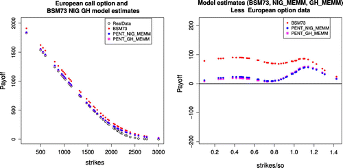
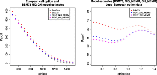
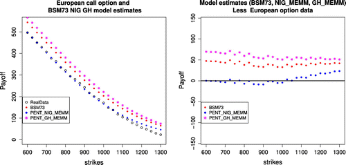
Once the parameters of discrete distributions are specified, pentanomial lattice building procedure is analogous to that of binomial lattices. Option values are obtained through a recursive procedure, and the corresponding graphical results presented in Figures 3, 4, 5.

Figure 3. S&P500 call options price, model comparison $S_t=2102$, $r=2.5\%$ p.a., $\mathit{\tau }\equiv T-t=431$ days.

Figure 4. RUT2000 European call options price, model comparison. $S_t=1073$, $r=2.5\%$ p.a., $T-t=320$ days.

Figure 5. RUI1000 European call options price, model comparison. $S_t=1117$, $r=2.5\%$ p.a., $T-t=455$ days.

4.2. European call option prices

A call option gives the owner the right, but not the obligation, to buy a particular security at a pre-specified price within a pre-specified time period. The value of such an option will be intimately related to the distribution of the price of the underlying instrument at the time of maturity. Specifically the more volatile the underlying price process, the more valuable the option. The standard approach for pricing options rely on risk neutral valuation methods. In this risk-neutralized probability measure, the price of a call option, that does not allow for early exercise and pays no dividends, will be qual to the discounted expected value of the payoffs at the maturity date. Our analysis is meant to illustrate a possibility of modeling volatility dependencies when calculating option prices.

To that end, we compare the performance of three lattice models for short time and long term maturity level at the money and out of the money European call options priced in Black and Scholes (1973) world, i.e.$$\begin{array}{cc}\hfill C^{BS}(t,K)& =S\mathrm{\Phi }(d_1)-K{e}^{-r(T-t)}\mathrm{\Phi }(d_2)\hfill \\ \hfill d_1& =\frac{ln(S_t/K{e}^{r(T-t)})}{\widehat{{\mathit{\sigma }}_H}\sqrt{T-t}}+\frac{1}{2}\widehat{{\mathit{\sigma }}_H}\sqrt{T-t}\hfill \\ \hfill d_2& =\frac{ln(S_t/K{e}^{r(T-t)})}{\widehat{{\mathit{\sigma }}_H}\sqrt{T-t}}-\frac{1}{2}\widehat{{\mathit{\sigma }}_H}\sqrt{T-t}\hfill \end{array}$$

where we let t refer to the present time and $\mathit{\tau }=T-t$ the time to expiry date in days. An option is said to be at the money if the exercise price, K, equal the current value of the underlying security. Lattices are calibrated in data generating process $\mathbb{P}$ and transformed to $\mathbb{Q}$ minimal entropy martingale measure. In all the models same parameters are used and results plotted against real market data and compared to Black Scholes model of 1973.

4.3. Empirical performance of the proposed model

The pricing performance of our model is tested relative to 200 European call options on the S&P500 index, RUT2000 index, and RUI1000 index at the close of the market on 11 April 2016. The data were taken from market watch website. On 11 April 2016,the closing price for the three indices (S&P500,RUT2000, RUI1000) were $S_t$= $2021,$1073, and $1117 respectively. We assumed general annual risk free rate of $r=2.5\%$ with no divided yield. We took long term options with maturities, 431, 320 and 455 days respectively. The performance evaluated based on real option prices of data of the proposed model is measured with three indicators: (i) the dollar root mean squared absolute error (RMSE), (ii) the average relative pricing error (ARPE) and (iii) the average absolute error (APE) given below.(4.2) $$\begin{array}{cc}\hfill RMSE(\mathrm{\$})& =\sqrt{\sum _{j=1}^N\frac{{(C_j^{market}-C_j^{model})}^2}{N}}\hfill \end{array}$$(4.2) (4.3) $$\begin{array}{cc}\hfill ARPE(\%)& =\frac{1}{N}\sum _{j=1}^N\frac{|C_j^{market}-C_j^{model}|}{C_j^{market}}\times 100\hfill \end{array}$$(4.3) (4.4) $$\begin{array}{cc}\hfill APE(\%)& =\frac{1}{N}\sum _{j=1}^N\frac{|C_j^{market}-C_j^{model}|}{\overline{C^{market}}}\times 100\hfill \end{array}$$(4.4)

where N represents the total number of options and $\overline{C^{market}}$ is the average option price. Table 4 summarizes the overall pricing errors of the various models considered here. We notice option prices computed based on pentanomial NIG lattice and Pentanomial GH lattice outperform the ones calculated based on BSM73 model for long term maturity days considered here as presented.

Table 4. European call option on 11 April 2016 Pricing performance under the three pricing kernels

Index	Pricing Kernel	$S_t$	N	$T-t$	$\overline{C^{\text{market}}}$	RMSE($)	ARPE(%)	APE(%)
S&P500		2102	40	431	576.74
	BSM73					78.25	181.91	13.37
	PENT-NIG					29.83	119.28	4.54
	PENT-GH					30.12	126.22	4.39
RUT2000		1073	21	320	190.85
	BSM73					25.49	91.63	12.98
	PENT-NIG					9.56	58.86	3.99
	PENT-GH					10.43	59.26	4.87
RUI1000		1117	29	455	222.44
	BSM73					40.55	37.42	18.12
	PENT-NIG					10.12	13.00	3.35
	PENT-GH					57.06	49.22	25.50

5. Conclusion

In this paper we establish the asset dynamics under the physical probability measure $\mathbb{P}$ in incomplete market, also apply minimal entropy martingale measure to change dynamics to risk neutral $\mathbb{Q}$. We assumed log-Lévy model to calibrate dynamics of the underlying price process and MEMM to change the historical probability risk neutral probability measure.

The valuation of contingent claims whose value depend on multiple sources of uncertainty is an important problem in financial economics. Since numerical methods for valuing such claims can be computationally expensive, the need for an efficient algorithm is clear. We made simplifying assumptions in that direction, even though there is more to be refined.

Although the pentanomial lattice provided in this article are tractable as the standard binomial, the pentanomial lattices approach, and may be extended to the multinomial case. Pentanomial lattices can be considered useful for relatively long term contracts (200 days and above) which can be used to solve American type options problems incorporating skewness and kurtosis. In depth study and more data sets are required to fine tune this observation.

Since option prices may react sensitively to changes in volatility, a proper specification of the conditional means at each step may play a crucial role in the proposed pentanomial model. Under the proposed framework, the market is in general incomplete, which is challenging to handle for the implication is a multitude of equivalent martingale measures and thus, a variety of no-arbitrage prices.

We note that under the proposed underlying dynamics, the proposed pricing model outperform bench mark model such as Black scholes model for the long term contract, pentanomial NIG lattice outperforms the other two models. We leave model refinement and extensions for future research. It would be interesting to incorporate changing volatility in the pentanomial framework and compare the result.

Acknowledgements

Financial support from the International Science Programme (ISP) Sweden in collaboration with the Eastern African Universities Mathematics programme, is greatly acknowledged. This article was fine tuned while visiting University of Cape town, South Africa as part of my post doctoral study invited by the African Collaboration for Quantitative Finance and Risk Research (ACQuFRR) directed by Prof. David Taylor. Thanks to the anonymous reviewer for his helpful corrections and suggestions.

Additional information

Funding

This work was supported by International Science program/EAUMP.

Notes on contributors

Ivivi J. Mwaniki

Ivivi J. Mwaniki completed his PhD at the University of Nairobi Kenya in collaboration with Uppsala University Sweden under East African Universities Mathematics Programme/International Science Programme. Currently he works for the University of Nairobi School of Mathematics. This article is part of the ongoing research in relation to option pricing in general. His research interest include option pricing, optimization, time series analysis and mixtures of various distributions, insurance and risk management.

References

- Barndorff-Nielsen, O. (1998). Process of normal inverse Gaussian type. Finance Stochastics, 2, 41–68.
- Black, F., & Scholes, M. (1973). The pricing of options and corporate liabilities. Journal of Political Economy, 81, 659–683.
- Carr, P., German, H., Madan, D., & Yor, M. (2002). The fine structure of asset returns: An empirical investigation. Journal of Business, 75, 305–332.
- Chan, W., & Maheu, J. (2002). Conditional jump dynamics in stock market returns. Journal of Business and Economic Statistics, 20, 377–389.
- Choulli, T. & Striker, C. (2006). More on minimal entropy-hellinger martingale measure. Mathematical Finance, 16(1), 1–19.
- Cont, R. (2001). Empirical properties of asset returns: Stylized facts and statistical issues. Quantitative Finance, 1, 223–226.
- Cox, J., Ross, S., & Rubinstein, M. (1979). Option pricing: A simplified approach. Journal of Financial Economics, 7, 229–264.
- Derman, E., & Kani, I. (1994). Implied trinomial trinomial trees of the volatility smile. Goldman Sachs quantitative strategies research notes.
- Duan, J., Ritchken, P., & Sun, Z. (2006). Approximating garch-jump models, jump-diffusion processes and option pricing. Mathematical Finance, 16, 21–52.
- Esche, F., & Schweizer, M. (2005). Minimal entropy preserves the lévy property: how and why. Stochastics and their Applications, 115, 299–327.
- Florescu, I., & Viens, F. (2008). Stochastic volatility: Option pricing using a multinomial recombining tree. Applied Mathematical Finance, 15, 151–181.
- Frittelli, M. (2000). The minimal entropy martingale measure and valuation problem in incomplete markets. Mathematical Finance, 10, 39–52.
- Fujiwara, T., & Miyahara, Y. (2003). The minimal entropy martingale measures for geometric lévy processes. Finance and Stochastics, 7, 509–531.
- Harrison, M., & Kreps, M. (1979). Martingales and arbitrage in multiperiod securities markets. Economic Theory, 20, 381–408.
- Harrison, M., & Pliska, S. (1981). Martingales and stochastic integrals in the theory of continous trading. Stochastic Processes and their Applications, 11, 215–260.
- Hsieh, D. (1989). Testing for nonlinear dependance in daily foreign exchanges rates. Journal of Business, 62, 339–368.
- Kamrad, B., & Ritchken, P. (1991). Multinomial approximating models for options with k state variables. Management Science, 37, 1640–1652.
- Kargin, V. (2005). Lattice option pricing by multidimensional interpolation. Mathematical Finance, 15, 635–647.
- Kellezi, E., & Webber, N. (2004). Valuing Bermudan options when the asset returns are Lévy processes. Quantitative Finance, 4, 87–100.
- McNeil, A., Frey, R., & Embrechts, P. (2005). Embrechts. Quantitative risk management: Concepts techniques and tools. Priceton University Press.
- Miyahara, Y. (2001). Geometric lévy process & memm: Pricing model and related estimation problems. Asia-Pacific Financial Markets, 8, 45–60.
- Nieuwland, F., Verschoor, W., & Wolff, C. (1994). Stochastic trends and jumps in ems exchange rates. Journal of International Money and Finance, 13, 699–727.
- Primbs, J., Rathianam, M., & Yamada, Y. (2007). Option Pricing with a pentanomial lattice model that incorporates skewness and kurtosis. Applied Mathematical Finance, 14, 1–17.
- Rendleman, R., & Bartter, B. (1979). Two state option pricing pricing. Journal of Finance, 3, 1093–1110.
- Ritchken, P., & Trevor, R. (1999). Pricing options under generalized GARCH and stochastic volatility process. Journal of Finance, 54, 337–402.
- Ssebungenyi, C. (2008). Valuation of real options using the minimal entropy martingale measure. Applied Mathematical Sciences, 2, 2875–2800.
- Ssebugenyi, C. S., Mwaniki, I. J., & Konlack, V. S. (2013). On the minimal entropy martingale measure and multinomial lattices with cumulants. Applied Mathematical Finance, 20, 359–379.
- Wu, C. (2006). The GARCH option pricing model: A modification of lattice approach. Review of Qantitative Finance and Accounting, 26, 55–66.
- Yamada, Y. & Primbs, J. (2001). Properties of multinomial lattice random walks for optimal hedges. International Conference of Computational Science, 579–588.
- Yamada, Y., & Primbs, J. (2004). Properties of multinomial lattices with cumulants for option pricing and hedging. Asia-Pacific Fianacial Markets, 11, 335–365.