Cross-sectional volatility index as a proxy for the VIX in an Asian market

Abstract

We present a cross-sectional volatility index (CSV) applied to an Asian market as an alternative to the VIX. One problem with the construction of a VIX-styled index is that it depends on the price of calls and puts, however, the CSV index may be applied to measure the volatility when no derivatives market exists. We formulate this volatility index based on observable and model-free volatility measures. We provide a statistical argument to support that an equally weighted measure of average idiosyncratic variance would forecast market return and show that this measure displays a sizable correlation with economic uncertainty.

Keywords:

• cross-sectional volatility index
• proxy VIX
• idiosyncratic risk
• GARCH forecast volatility

Public Interest Statement

We present a cross-sectional volatility index (CSV) applied to an Asian market as an alternative to the VIX. The purpose of this study is to propose appropriate volatility indices and volatility-based derivative with its foundation focusing on crucial methodology on less liquid markets in Asia. One problem with the construction of a VIX-styled index is that depends on the price of calls and puts, however, the CSV index may be applied to measure the volatility when no derivatives market exists. The volatility measurement has model-free nature and it is flexible enough to apply to any region, sector and style of the world equity markets in any frequencies. We provide statistical argument to support that an equally weighted measure of average idiosyncratic variance would forecast market return and show that this measure displays a sizable correlation with economic uncertainty.

1. Introduction

The VIX is a widely accepted measure of the level of volatility in the developed markets. However, this index does have a number of limitations, especially in relation to Asian markets under review. The calculation of a VIX-styled index depends on a vibrant derivative market. In less developed markets, where the derivative market is illiquid or non-existent, it becomes inappropriate to use this approach. In such cases, we propose to use a CSV methodology as a measure of volatility level. The CSV index is a recent form of measure associated with volatility, see Goltz, Guobenzaite, and Martellini (2011) for details. CSV is another way to attain the stock markets’ co-movement and global risk measurement. The construction of the CSV is quite distinction from the VIX. Ahoniemi (2006) demonstrate the VIX calculation to forecast the future by directional accuracy and estimating the profitability of the trades. Few Asian markets have a vibrant derivatives sector to supply the necessary inputs to calculate a VIX-styled index. The method is based on observable and model-free volatility measures of all data and frequencies. This new form of index provides a good approximation of average idiosyncratic variance. The technical foundations of the new form indices have been defined by Garcia, Mantilla-Garcia, and Martellini (2011). The results of the new form of volatility index can be used as a reliable proxy when such measures of volatility are not available.

The idiosyncratic volatility has also been of interest among researchers. Nartea, Ward, and Yao (2011) and Campbell, Lettau, Malkiel, and Xu (2001) show how idiosyncratic volatility benefited diversification. In this article, we test the validity of the CSV index by showing the measure is strongly correlated to the performance of the VIX. This is important as we wish to show that the CSV index can be used as a reliable proxy in a VIX-styled market without a local derivatives market. So, in this study, we will develop a volatility index based on model-free implied volatility. As an illustration, we shall apply the method to the Japanese market. Therefore, in subsequent work, we expand the method into developing countries. The purpose of this study is to propose appropriate volatility indices and volatility-based derivative with its foundation focusing on crucial methodology in less liquid markets in Asia. One of the reasons for choosing this method is because the volatility measurement has a model-free nature and is flexible enough to apply to any region, sector and style of the world equity markets in any frequencies. Another advantage of this method is that with the model, there is no need to resort to any auxiliary option market.

A volatility measures have been the main focus among researchers and policy-makers. Less attention has been given to CSV of the dispersion of stock returns. There are two forms of volatility measures: systematic and unsystematic. For instance, Ang, Hodrick, Xing, and Zhang (2006) discuss systematic volatility as a measure on the sensitivity of the variation in stock returns. However, unsystematic volatility is measured by residual variance of stocks in a specific period of time by the use of error terms. A study of the systematic volatility can be found in Cutler, Katz, Sheiner, and Wooldridge (1989). Previous studies have focused on the GARCH model as a volatility model. Due to information content, the bias, the efficiency forecast of the predictor, a GARCH model can be employed to examine and compare with other volatility models, see Bentes (2015) for more details. Besides that, Bagchi (2016) suggests that the dynamic relationship between the stock price volatility and exchange rate volatility in India exist by the extension of GARCH namely, asymmetric power ARCH(APARCH) model is applied.

When using implied volatility to construct the VIX index, the standard deviation is estimated on its volatility of security prices. For example, as experienced by the South African market, only recently has the market had access to the information content in SAVI implied volatility, see Kenmoe and Tafou (2014). Kenmoe and Tafou (2014) mention that once all information contents are retrieved, essentially the options price, then one can compute stock’s market volatility equation option price and the pricing model. The information on option prices is available in more developed countries. This is the reason that researchers intend to carry out further studies on volatility in more liquid markets of the developed world (Ang et al., 2006; Garcia et al., 2011; Goltz et al., 2011). Apart from this, as mentioned in Siriopoulos and Fassas (2012), less emergent countries have established derivative markets, but many are without this dimension.

Many Asian derivative markets are still in the early stages of development compared to the Western market, as surveyed by Hohensee and Lee (2006). The transparency and liquidity of the underlying markets are the fundamental success factors for derivatives market. However, the derivative market in many Asian countries is either non-existent or in the early stages of development; and so unsuitable for a VIX-like index.

The contribution of this paper to the literature is threefold. Firstly, we introduce and examine the CSV approach as a new form of volatility index in the US market. This, in turn, allows us to obtain consistent estimates of parameters of the financial market model using a single cross section of return data for the Japanese market. This CSV index approach is a measure that is observable and has a model-free nature that is available for every region, sector and style of the world equity markets. We show that a cross-sectional measure provides a good approximation of average idiosyncratic variance. Secondly, we show that the new form of volatility index in the Japanese market is an efficient benchmark index providing the cross-sectional variance returns are the average idiosyncratic variance of stocks within the Asian countries. Additionally, the measure is different from the historical volatility and implied volatility as it is available for every region, sector and style of world equity markets. Thirdly, we test the forecast capabilities of the CSV in the market that has a lack of derivatives options. This is to measure its performance against the VIX.

1.1. Outline

The remainder of this paper is organised as follows; Section 1 gives an account of previous works. Section 2 describes the methodology and research model, the GARCH models, the Volatility measures and forecasting measurements used to construct the cross-market volatility index. Section 3 describes the data used in this paper. Our new results are described in Section 4. Finally, Section 5 gives the conclusions.

2. GARCH model with cross-sectional market volatility

The CSV indirectly describes the changes in the environment driven by country,¹ stock behaviour and sector selection. In Ankrim and Ding (2002), it is shown that the model depends largely on intertemporal measures. This relates to variability of daily, monthly or quarterly returns for a market of a long horizon. There are also three factors that are combined to generate an expected change of CSV. The factors are the change in the average volatility in the sectors making up the market, the change in overall market volatility and the change in the sector mean dispersion. The classical CSV method is based on a statistically robust estimation due to unexpected outliers.

Assumptions by Garcia et al. (2011) state that the cross-sectional measure of variance provides a good approximation for average idiosyncratic variance of a given universe of stock. The stock returns $r_{it}$ are modelled as follows:(1) $$\begin{array}{c}\hfill r_{it}={\mathit{\beta }}_{it}{F}_t+{\mathit{\epsilon }}_{it}\end{array}$$(1)

where $F_t$ is the factor at time t, ${\mathit{\beta }}_{it}$ is the beta of stock i at time t, and ${\mathit{\epsilon }}_{it}$ is the residual or specific return on stock i at time t, with $E({\mathit{\epsilon }}_{it})=0$ and $\text{cov}(F_t,{\mathit{\epsilon }}_{it})=0$. A strict factor model is assumed as $\text{cov}({\mathit{\epsilon }}_{it},{\mathit{\epsilon }}_{jt})=0$ for $i\ne j$. In a strict factor model, the idiosyncratic returns are assumed to be uncorrelated with one another. This is where the covariance matrix of idiosyncratic risks is a diagonal matrix. The idiosyncratic variance measurement over asset i is obtained by computing the residuals of the regression of ${\mathit{\sigma }}_i^2=\frac{1}{T}{\sum }_{t=1}^T{\mathit{\epsilon }}_{it}^2$. So, there are two main advantages of CSV idiosyncratic measurement. Firstly, the observed return can be computed directly and secondly, within any universe of stocks it is readily available at any frequency. When it can be computed directly, it means that no other parameters, such as betas, need to be estimated first. As to see this, let ${(w_t)}_{t\ge 0}$ be given weight vector process and then the return $r_t^{(w_t)}$ will be written as:(2) $$\begin{array}{c}\hfill r_t^{(w_t)}=\sum _{i=1}^{N_t}{w}_{it}{r}_{it},0<w_{it}<1\forall i,t,\end{array}$$(2)

where $N_t$ represents the total number of stocks at day t, and assume no loss of generality a conditional single factor model for excess stock returns. So, for all $i=1,\dots ,N_t$, the stocks are written in terms of the excess of the risk-free rate. Based on the assumptions outlined in the study of Garcia et al. (2011), the cross-sectional variance measure is defined as:(3) $$\begin{array}{c}\hfill {\text{CSV}}_t^{(w_t)}=\sum _{i=1}^{N_t}{w}_{it}{(r_{it}-r_t^{(w_t)})}^2\end{array}$$(3)

An equally weighted CSV is denoted as follows:(4) $$\begin{array}{c}\hfill {\text{CSV}}_t^{\text{EW}}=\frac{1}{N_t}\sum _{i=1}^{N_t}{(r_{it}-r_t^{EW})}^2\end{array}$$(4)

where $r_t^{\text{EW}}$ denotes the return of an equally weighted portfolio and the corresponding to the weighting scheme $w_{it}=1/N_t\forall i,t$.

This assumption is important as it draws a formal relationship between the dynamics of cross-sectional dispersion of realised returns and the dynamics of idiosyncratic variance. The assumption in Equation (3) is that the variance of the equally weighted CSV for a specific variance will disappear in the limit of an increasingly large number of stocks.²

The CSV Index has a model-free nature, so there is no need to specify a particular factor model to compute it. For instance, the study by Garcia, Mantilla-Garcia, and Martellini (2014) explains the feature model is model-free and there is no need to obtain residuals from other models to compute this model. Also, the corresponding cross-sectional measure is readily computable at any frequency from observed returns.

Xu and Malkiel (2004) and Merton (1987) have assumed that idiosyncratic risk is positively correlated with expected stock returns in the cross section. Idiosyncratic risk has little or no correlation with the market risk which may be eliminated from a portfolio using sufficient diversification. As in Garcia et al. (2011), we simplify the situation by introducing into the two following assumptions:

(1)	Homogeneous beta assumption: ${\mathit{\beta }}_{it}={\mathit{\beta }}_t,\forall i$.
(2)	Homogeneous residual variance assumption: $E({\mathit{ϵ}}_{it}^2)={\mathit{\sigma }}_{\mathit{ϵ}}^2(t),\forall i$.

In accordance with Garcia et al. (2011), as the number of constituents increases, the cross-sectional variance convergences to a specific limit. In other words, we have(5) $$\begin{array}{c}\hfill {\text{CSV}}_t^{(w_t)}=\sum _{i=1}^{N_t}{w}_{it}{(r_{it}-r{{}_t}^{(w_t)})}^2\underset{N_t\to \infty }{⟶}{\mathit{\sigma }}_{\mathit{ϵ}}^2(t)\end{array}$$(5)

where $N_t$ is the number of increasing constituents of the stock index market for a given date t, $r_t^{(w_t)}$ is the weighted return with weights $w_{it}$ at time t and ${\text{CSV}}_t^{(w_t)}$ is the cross-sectional variance.

Consequently, this gives a formal relationship between the cross-sectional dispersion and the idiosyncratic variance. The following equation shows the equally weighted ${\text{CSV}}_t^{(w_t)}$ as the best estimator for idiosyncratic variance within the class of CSV estimators under a positive-weighting scheme:(6) $$\begin{array}{cc}\hfill E[{\text{CSV}}_t^{(w_t)}]& ={\mathit{\sigma }}_{\mathit{ϵ}}^2(t)\left(1-\sum _{i=1}^{N_t}{w}_{it}^2\right)\hfill \end{array}$$(6) (7) $$\begin{array}{cc}\hfill \text{Var}[{\text{CSV}}_t^{(w_t)}]& =2{\mathit{\sigma }}_{\mathit{ϵ}}^2(t)\left({\left(\sum _{i=1}^{N_t}{w}_{it}^2\right)}^2+\sum _{i=1}^{N_t}{w}_{it}^2-2\sum _{i=1}^{N_t}{w}_{it}^3\right).\hfill \end{array}$$(7)

Equation (2) implies that ${\text{CSV}}_t^{(w_t)}$ is a biased estimator of the idiosyncratic variance. The bias estimator is given by the multiplicative factor $\left(1-{\sum }_{i=1}^{N_t}{w}_{it}^2\right)$ which can be corrected since it is available in explicit form. This equation may be extended to the case where the equally weighted scheme EW shows the bias and variance of the ${\text{CSV}}_t^{(w_t)}$. This equally weighted ${\text{CSV}}_t^{(w_t)}$ is among the best estimators when it is composed of positively weighting estimators. It has been shown that the bias and variance of $CS{V}_t^{(w_t)}$ is minimal for an equally weighted (EW), corresponding to $w_{it}=\frac{1}{N_t}$ of every date t. So, when the number of stocks grows large, this bias disappears and the variance tends to be zero for the EW scheme. However, the asymptotic result that holds for any weighting scheme has improved to a finite number of constituents $N_t$. It is explained in the following proposition.(8) $$\begin{array}{c}\hfill E[{\text{CSV}}_t^{\text{EW}}]={\mathit{\sigma }}_{\mathit{ϵ}}^2(t)\left(1-\frac{1}{N_t}\right)\underset{N_t\to \infty }{⟶}{\mathit{\sigma }}_{\mathit{ϵ}}^2(t)\end{array}$$(8) (9) $$\begin{array}{c}\hfill \text{Var}[{\text{CSV}}_t^{\text{EW}}]=2{\mathit{\sigma }}_{{\mathit{ϵ}}_t}^2\left(\frac{N_t-1}{N_t^2}\right)\underset{N_t\to \infty }{⟶}0.\end{array}$$(9)

Normally, average idiosyncratic variance will be used to calculate the beta of each stock portfolio where beta is the co-movement of an asset within the market.³ Hence, we can evaluate the market risk of a portfolio and the market variance. However, by adopting the CSV, it gives two advantages. The first advantage is that we can directly compute from the observed returns excluding beta as the parameters at any frequency. The second advantage is that the model is a nature-free model as we do not need to specify a particular model in order to compute it.

Even when a larger number of stocks are computed, the bias may still be small as CSV appears to be a biased estimator for average specific variance, especially when the homogenous beta does not apply. Empirically, it was shown by Garcia et al. (2011) that the value of the median from a sample period between July 1963 and December 2006 is small. As discussed in Goltz et al. (2011), the assumption of homogeneous residual variances and homogeneous beta is as follows:(10) $$\begin{array}{c}\hfill E[{\text{CSV}}_t^{\text{EW}}]=\left(\frac{1}{N_t}\sum _{i=1}^{N_t}{\mathit{\sigma }}_{\mathit{ϵ}i}^2(t)\right)\left(1-\frac{1}{N_t}\right).\end{array}$$(10)

After a straightforward simplification of the homogeneous beta assumption, for ${\mathit{\beta }}_{it}={\mathit{\beta }}_t$, we may write Equation (10) as:(11) $$\begin{array}{c}\hfill E[{\text{CSV}}_t^{\text{EW}}]=\left(\frac{1}{N_t}\sum _{i=1}^{N_t}{\mathit{\sigma }}_{\mathit{ϵ}i}^2(t)\right)\left(1-\frac{1}{N_t}\right)+F_t^2{\text{CSV}}_t^{\mathit{\beta }}\end{array}$$(11)

where(12) $$\begin{array}{c}\hfill {\text{CSV}}_t^{\mathit{\beta }}=\frac{1}{N_t}\sum _{i=1}^{N_t}{\left({\mathit{\beta }}_{it}-\frac{1}{N_t}\sum _{i=1}^{N_t}{\mathit{\beta }}_{it}\right)}^2\end{array}$$(12)

So the expected return is computed as an unbiased estimator which is the CSV as follows:(13) $$\begin{array}{c}\hfill {\text{CSV}}_t=\sqrt{\frac{\sum _{i=1}^{N_t}{(r_{it}-{\overline{r}}_t^{\text{EW}})}^2}{N_t-1}}\end{array}$$(13)

where ${\overline{r}}_t^{\text{EW}}$ represents the return of equally weighted stocks at date t and $N_t$ is the number of constituents in each of the stock markets.

2.1. GARCH volatility measures

The GARCH model in its simplest form proves that conditional variances can be estimated easily while giving parsimonious models than the ARCH model. The feature of GARCH explains a great predictive power with minimum number of parameters. It is widely employed by many researchers to predict variance using GARCH specification asserts in the next period. A study by Su (2010) estimates financial volatility of daily returns extracted in the Chinese stock market. GARCH and E-GARCH have been employed to fit the sample of the data and it is suggested that E-GARCH fits better than the GARCH model. GARCH has also been a model used to forecast the volatility of the Shanghai and Shenzen composite stock indices. The study examined how specifications of return distribution influence the forecast performance, see Liu, Lee, and Lee (2009). When forecasting the volatility performance of the VIX and CSV, we use the GARCH(p,q) by computing;(14) $$\begin{array}{cc}& r_t=\mathit{\mu }+{\mathit{\epsilon }}_t\hfill \end{array}$$(14) (15) $$\begin{array}{cc}& {\mathit{\epsilon }}_t={\mathit{\eta }}_t\sqrt{h_t}\hfill \end{array}$$(15) (16) $$\begin{array}{cc}& h_t=\mathit{\omega }+\sum _{i=1}^p{\mathit{\alpha }}_i{\mathit{\epsilon }}_{t-1}^2+\sum _{j=1}^q{\mathit{\beta }}_j{h}_{t-j}\hfill \end{array}$$(16)

where $r_t$ is the stocks return, $\mathit{\mu }$ is constant parameter; ${\mathit{\eta }}_t$ are i.i.d with $E({\mathit{\eta }}_t)=0$ and $\text{Var}({\mathit{\eta }}_t)=1$; ${\mathit{\eta }}_t$ is independent of $h_t$; $\mathit{\omega }>0,{\mathit{\alpha }}_i\ge 0$ and ${\mathit{\beta }}_j\ge 0$ are non-negative constants with ${\sum }_{i=1}^p{\mathit{\alpha }}_i+{\sum }_{j=1}^q{\mathit{\beta }}_j>1$ to ensure the positive of conditional variance and stationary as well. If $q=0$, the model reduces to an autoregressive conditional heteroscedasticity (ARCH) model.

We have chosen the E-GARCH because it is an extension to the GARCH model which allows us to observe the symmetric effects of positive and negative asset returns. See Brandt and Jones (2006) for further illustration. There are two limitations that make the GARCH and E-GARCH different. The limitation of the model assumes that only the magnitude of unanticipated excess returns determines $log({\mathit{\sigma }}_t^2)$. Another limitation is the persistence of volatility shock. The E-GARCH model is specified as:(17) $$\begin{array}{c}\hfill log({\mathit{\sigma }}_t^2)=\mathit{\omega }+\sum _{i=1}^p{\mathit{\alpha }}_i\left|\frac{u_{t-i}}{{\mathit{\sigma }}_{t-i}}\right|+\sum _{j=1}^q{\mathit{\beta }}_{j}log({\mathit{\sigma }}_{t-j}^2)+\sum _{k=1}^r{\mathit{\gamma }}_k\frac{u_{t-k}}{{\mathit{\sigma }}_{t-k}}\end{array}$$(17)

where $\mathit{\omega },\mathit{\alpha },\mathit{\beta },\mathit{\gamma }$ and $\mathit{\lambda }$ are coefficients, and $log({\mathit{\sigma }}_t^2)$ comes from a generalised error distribution. Using this model, we can expect a better estimate the volatility for asset returns due to how the E-GARCH counteracts the limitations on the classic GARCH model, See Engle and Patton (2001).

2.2. Forecasting volatility measures

To determine the efficiency of the CSV approach, a forecast of both VIX and the CSV index has been generated to estimate the volatility errors. We have used the finite sample scale-sensitive performance criteria which is the root mean square error (RMSE), the mean absolute error (MAE) and the Theil Inequality Coefficient (U2). The RMSE is calculated as follows:(18) $$\begin{array}{c}\hfill \text{RMSE}=\sqrt{\frac{1}{T}\sum _{t=1}^T{\left({{\widehat{\mathit{\sigma }}}_t}^2-{\mathit{\sigma }}_{{}_t}^2\right)}^2}\end{array}$$(18)

where ${{\widehat{\mathit{\sigma }}}_t}^2$ is the forecasted volatility at time t, and ${\mathit{\sigma }}_t$ is the actual CSV volatility at time t and T is the sample size. The MAE is dependent on the scale of the dependent variable but is less sensitive to large deviations than the usual squared loss which is(19) $$\begin{array}{c}\hfill \text{MAE}=\frac{1}{T}\sum _{t=1}^T\left|{{\widehat{\mathit{\sigma }}}_t}^2-\mathit{\sigma }{{}_t}^2\right|.\end{array}$$(19)

The benchmark forecast value of the last observations appears to be the Theil Inequality Coefficient which is the earliest relative forecast accuracy measure. It is scale invariant and lies between zero and one. However, if the Theil coefficient is equal to zero, then it is a perfect fit. We have(20) $$\begin{array}{c}\hfill U2=\frac{{\sum }_{t=1}^T{\left({{\widehat{\mathit{\sigma }}}_t}^2-{\mathit{\sigma }}_t^2\right)}^2}{{\sum }_{t=1}^T{\left({\mathit{\sigma }}_{t-1}^2-{\mathit{\sigma }}_t^2\right)}^2}\end{array}$$(20)

where ${{\widehat{\mathit{\sigma }}}_t}^2$ is the forecasted volatility at time t, ${\mathit{\sigma }}_t$ is the actual volatility at time t and T is the sample size.

3. Data and the construction of volatility and control variables

We employ all stocks included in the S&P 500 and NIKKEI-225 index during the period from October 2004 to September 2014.⁴ This period of this data can only retrieved at this range due to limited index data from the VXJ. The VXJ is a new model based on the new VIX methodology developed by Fukasawa, Ishida, Maghrebi, Oya, Ubukata, and Yamazaki (2011) as a model-free index of market volatility implicit in the bid and asked prices of NIKKEI-225 options traded at the Osaka Securities Exchange. So, we obtain the daily time series of the CBOE VIX and Japanese VXJ obtained from Bloomberg database for the same period as the stock index. We use the daily returns to estimate the idiosyncratic volatility following the approach of CSV as a proxy for the classic VIX index. Table 1 shows the descriptive statistics on the volatility index measures.

Table 1. Descriptive statistics on volatility return index measures sample period (2004–2014)

Measure	CBOE VIX	S&P 500 CSV	VXJ	NIKKEI-225 CSV
Mean	0.0023	0.0258	0.0021	0.0209
Median	$-0.0052$	$-0.0015$	$-0.0038$	$-0.0063$
Maximum	0.6421	1.6997	0.7826	4.3323
Minimum	$-0.2957$	$-0.5779$	$-0.3089$	$-0.5502$
Std. deviation	0.0705	0.2412	0.0670	0.2257
Skewness	0.6862	0.1750	1.5262	0.3392
Kurtosis	7.2681	3.7917	14.8883	5.7385
Jarque-Bera	5,584.2981	2,208.9521	58,242.1700	323,686.1000
Observation	2429	2429	2519	2519

Table 1 presents the sample size, unconditional mean, unconditional variance, skewness, excess kurtosis and the Jarque-Bera test statistic. The CBOE VIX and the CSV index have a small mean value. It reflects on the average of the volatility return for both models. It shows that the daily volatility is more volatile in CSV compared to the CBOE VIX. The returns have a small skewness and a high kurtosis. The highest kurtosis is the return index of NIKKEI-225 using CSV index model which is 14.88.

Table 2 reports the descriptive statistics of the volatility index for both US and Japanese markets. Firstly, the of oft-noted tendency of implied volatility to overestimate actual volatility is reflected in that the mean implied volatility is 19.97%, while the annualised standard deviation of the CSV S&P 500 index is 13.1% as calculated from the daily returns. Secondly, the volatility index for both implied volatility and the CSV are positively serially correlated and the level of the index in the best of range (less than 30% per annual). Thirdly, the VXJ is more volatile than the CSV NIKKEI-225 with an annualised standard deviation of daily log percentage changes of 10.91%. Both of the implied and CSV are highly positively correlated with correlations of 0.63 and 0.77.

Table 2. Descriptive statistics of implied volatility index and CSV index

Series	Mean	Standard deviation	Correlation	Daily returns (annualised)
CSV NIKKEI-225 index-levels	26.72	9.79	0.6293	2429
VXJ levels	25.28	10.91	0.6293	2429
CSV S&P 500 index-levels	26.25	13.01	0.7693	2519
VIX levels	19.97	9.99	0.7693	2519

Table 3. Correlation matrix analysis of volatility return index

Correlation	CBOE VIX	S&P 500 CSV	VXJ	NIKKEI-225 CSV
CBOE VIX	1	0.7662	0.5203	0.3607
S&P 500 CSV		1	0.53	0.4016
VXJ			1	0.6294
NIKKEI-225 CSV				1

Table 3 indicates that the CBOE VIX index approach model has a strong positive correlation with the CSV model of S&P 500. This is also the same for NIKKEI-225 which has high correlations between the VIX and CSV index approaches. Here, it indicates that the CSV index may have a potential proxy for VIX index essentially on non-derivatives market. This is because it shows a high correlation between the CBOE VIX and the new form of volatility index approach, the CSV index.

We extract daily components of S&P 500 and NIKKEI-225 price returns to construct a CSV to measure the idiosyncratic risk. The sample period is from October 2004 to September 2014. The number of firm from each component varies from 300 to 500. Illiquid stocks have been filtered out from the data. There are a few constituent stock returns from S&P 500 and NIKKEI-225 that have been removed. The outliers of the removed stocks are the stocks that have extreme return movements throughout the time period. Illiquid stocks that are identified as stocks with⁵ stale prices, for instance indicating zero returns over a given day, high first-order autocorrelation as well as abnormal values for other common liquidity measures including trading volume. The new construction of volatility index will perform a greater robustness of the constructed risk measure. We have generated a sample from the period ranging from October 2004 to September 2014 in Table 3 and the results generated are quite consistent and the volatility returns index are highly correlated.

There are formal tests to examine whether the CSV index approach produces significant results to proxy the CBOE VIX. This is achieved using the GARCH-type model to determine first whether the CSV index is indeed a good predictor of volatility. Also, we can see whether the CSV index is a better predictor than the alternative measures of volatility. It predicts the period’s variance by looking at the weighted average of the long-term historical variance. It gives parsimonious models that are easy to estimate, even in its simplest form; this has proven surprisingly successful when predicting conditional variances. The data employed for the forecast performance measure are the CSV and the VIX daily index for the US and Japanese markets. The data are divided into two subsets. The first subset is called the in-sample data-set and is built up model for the underlying data and the second subset is called the out-sample data-set used to investigate the performance of volatility forecasting. The in-sample data-set analysis starts from 2004 to 2013 and out-sample data-set is from 2013 to 2014. Here we evaluate the forecast performance with 2,430 observations. We forecast the performance of volatility using a GARCH and E-GARCH model.

4. Empirical analysis

4.1. The behaviour of the market volatility index

We examine the daily CBOE VIX index for sample periods running from 4 October 2004 to 3 October 2014. The total daily observations are 2,519. Figure 1 plots the time series of the VIX during the particular sample period. It seems that the VIX tends to oscillate in long swings between a quite volatile regime with high index values and a more stable regime with low index values. According to Figure 1, high volatility characterises the periods ranging from September 2008 to May 2009. This is the year of the massive financial crash in the market and the inevitable financial chaos is consequently reflected in the VIX. The collapse of Lehman would also be the main reason for the high volatility in the VIX in 2008 and the subsequent credit crunch and global financial crisis. In contrast, low volatility seems dominant from October 2004 to August 2008 and from June 2009 to October 2014. It is consistent with the claim in Whaley (2000), that one may interpret the VIX as the investors fear gauge.

Figure 1 shows a high correlation of 0.77 between the CBOE VIX and the S&P 500 CSV index based on the correlation test in Table 3. The sample period runs from 4 October 2004 to 3 October 2014. This suggests the average idiosyncratic volatility counterpart is close to the option implied volatility, due to the strong relationship between the two models exhibit. It seems that a high correlation exists in the return index due to the condition of market changes, with a correlation that tends to be higher in down markets. The pattern of the volatility using the VIX approach is almost the same where the spikes move together.

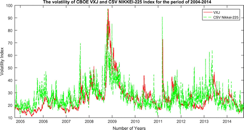
Figure 1 also demonstrates the volatility of S&P 500 using the second approach; the CSV. The volatility fluctuates decidedly when it reaches the same period with the CBOE VIX and the trend of the volatility seems to move together. The CSV index value reaches the peak at 123.1017 in November 2008 whereas the CBOE VIX has an index value of 64.7. Then both measures simultaneously continue to display high volatility. When these readings are high in the VIX or CSV index, the mark periods on higher stock market volatility tend to move in same direction with the stock market bottom. Figure 2 shows the VXJ and the CSV of NIKKEI-225 volatility movement and the correlation is also high and positive with the value of 0.62. Both models exhibit the movement of volatility and it results that they coordinately move together with the average dispersion at 15.80. The volatility index of cross-sectional method has a lower index compared to the Japanese VXJ. We confirm this intuition by reporting the high correlation between the VIX index and the corresponding CSV index based on the S&P 500 and NIKKEI-225 universe. The correlation test is an important measure of unsystematic risk-based option prices and the CSV index which is a model-free, efficient and unbiased proxy for specific risk. By proposing the CSV in Japan as an alternative to measure risk in an Asian markets, the volatility of the index is more certain and stable compared to the Japanese VIX initiated by the CBOE VIX in the United States. We could see that there is a sharp increase of the index value in the CBOE VXJ from July 2008 to October 2008 in the figure. Although low volatility is still consistent throughout the time period after a slight period of high spikes averaging an index value of 25.28, albeit still under the value index 30. Figure 2 also illustrates the volatility of NIKKEI-225 using CSV approach. It shows a stable index value and the index value runs along together smoothly with the Japanese VXJ approach.

Figure 1. The volatility of CBOE VIX and the cross-sectional volatility index for the sample period of 2004–2014.

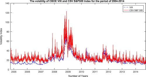
Figure 2. The volatility between the Japan CBOE VIX and the NIKKEI-225 Cross-Sectional Volatility Index for the sample period of 2004–2014.

We have also run an analysis of a 252-day rolling window correlation to provide a further co-movement check between the VIX and the CSV for both markets in the US and Japan. The results suggest that the correlation of the two returns series fluctuates and are inconsistent within the sample period from 2004 to 2014. Figures 3 and 4 show the 252-day rolling window correlation. The bigger the size of the window, the more certain and stable the correlation will be. However, Figure 3 illustrates the rolling window correlation between the CBOE VIX and CSV index. The volatile correlation surged during the financial crisis. There is a similar trend between Figures 3 and 4 when comparing the rolling correlation’s standard deviation amongst each other. It seems that both figures show a sharp drastic correlation downwards and an upward trend in the years 2007, 2008 and 2010. It shows the significant relationship between the CBOE VIX and the CSV index approach.

Figure 3. Two hundred fifty two days rolling window correlation of VIX and CSV S&P 500.

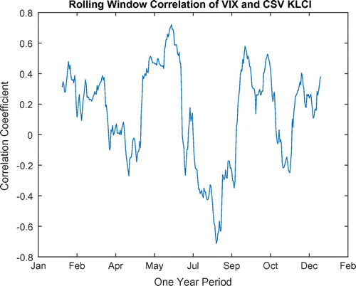
Figure 4. Two hundred fifty two days rolling window correlation of VXJ and CSV NIKKEI-225.

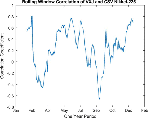
Table 4 describes the estimate of conditional volatility measures for the GARCH and E-GARCH of the CBOE VIX and CSV index approaches for both markets namely in the US and Japanese. We model the conditional volatility as being a GARCH(1,1) process. The specification would show a parsimonious representation of conditional variance that adequately fits many high-frequency time series. The GARCH and E-GARCH models represent the estimation for the return series of 500 stocks in the US and 225 stocks in Japan. From the observations, the size of the parameters $\mathit{\alpha }$ and $\mathit{\beta }$ determine the short-run dynamics of the resulting volatility time series. Most of the parameter estimates in Table 3 are statistically significant at a 5% level. The GARCH results indicate the persistence in volatility with $\mathit{\alpha }$ and $\mathit{\beta }$ ranging from 0.72 to 0.93 which is closer to 1.00. This suggests a stronger presence of ARCH and GARCH effects towards the CSV S&P 500, Japanese VXJ and CSV NIKKEI-225. The E-GARCH is applied to examine the asymmetric effects of volatility and coefficients of the asymmetric effect. The parameter $\mathit{\gamma }$ shows the leverage effects and from the observation, the effects are mostly positive at a significance level of 5%.

Table 4. The estimation of conditional volatility measures of GARCH/EGARCH

	GARCH(1,1)				EGARCH(1,1)
	CBOE VIX	CSV S&P 500	Japan VXJ	CSV NIKKEI-225	CBOE VIX	CSV S&P 500	Japan VXJ	CSV NIKKEI-225
Constant	0.0060*	0.0083*	0.0003*	0.0095*	$-0.3334$*	$-0.6771$*	$-0.4964$*	$-1.0700$*
$\mathit{\alpha }$	$-0.4710$	0.06501*	0.1465*	0.0920*	0.0625*	0.1330*	0.1258*	0.1829*
$\mathit{\beta }$	0.7293*	0.7432*	0.7870*	0.6298*	0.1784*	0.03060	0.2031*	0.03312
$\mathit{\gamma }$	–	–	–	–	0.9467*	0.8181*	0.9281*	0.7259*

*Statistically significant level of 0.05 percent.

Table 5. The volatility forecast error with different approach of GARCH model

	GARCH(1,1)				EGARCH(1,1)
	CBOE VIX	CSV S&P 500	Japan VXJ	CSV NIKKEI-225	CBOE VIX	CSV S&P 500	Japan VXJ	CSV NIKKEI-225
Root mean square error (RMSE)	0.0872	0.1693	0.0714	0.1600	0.1005	0.1689	0.0714	0.1602
Mean absolute error	0.0723	0.1410	0.0409	0.1322	0.0780	0.1406	0.0415	0.1323
Theil inequality coefficient	0.5958	0.6553	0.9178	0.6621	0.9676	0.6551	0.9296	0.6613
Bias proportion	0.0000	0.0425	0.0006	0.0038	0.0313	0.0374	0.0008	0.0056
Variance proportion	0.4563	0.4611	0.8522	0.3722	0.9586	0.4655	0.8822	0.3689
Covariance proportion	0.5437	0.4694	0.1472	0.6241	0.0101	0.4970	0.1170	0.6255

Table 5 provides results of forecast error statistics for each model according to symmetric error measures of the two stock markets: S&P 500 and NIKKEI-225. Results of the RMSE and MAE criteria suggest that GARCH is the best performing model compared to E-GARCH for the CBOE VIX and VXJ. On the other hand, the E-GARCH provides the worst forecast for the NIKKEI-224 and S&P 500 CSV index. However, considering the Theil Inequality Coefficient criteria, it seems that the CSV index for both S&P 500 and NIKKEI-225 perform better in E-GARCH. The forecast error statistics are employed to compare the performance of VIX and the CSV index approaches. The use of RMSE is to help provide a complete picture of the error distribution when forecasting the volatility of the VIX and CSV index. The RMSE and the mean absolute error (MAE) are very small when using the CSV Index and the VIX approach methods. The smaller the values of MAE and RMSE, the more accurate, on average, the forecast of a model. The smaller the value of the U-Theil, the better the model performs compared to a naive forecast with no change. Therefore, the most accurate forecast is based on the mean absolute error criteria for the two models which are the GARCH and E-GARCH. This reflects on whether the CSV index approach could possibly a proxy of the CBOE VIX approach.

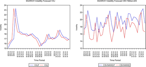
Figures 5–8 show the performance of volatility forecasts of the VIX and CSV for both the US and Japanese markets based on the GARCH and E-GARCH volatility model. The red legend shows the actual CSV volatility whereas the blue legend describes the GARCH or E-GARCH prediction volatility. The observations from the figures are made using the sample prediction from 3 September 2014 to 3 October 2014. The actuals and predictions for each of the VIX and CSV volatility approaches are quite persistent and may have a significant influence on volatility. As to compare the two methods of GARCH and EGARCH volatility model, it appears that the GARCH has a better forecast for a volatility model for both the CSV and VIX models as these may be seen from the size of the gap.

Figure 5. Volatility forecast of VIX and cross-sectional volatility index (CSV) using GARCH in US market.

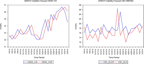
Figure 6. Volatility forecast of VXJ and cross-sectional volatility index (CSV) using EGARCH in the US market.

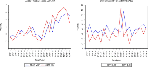
Figure 7. Volatility forecast of VXJ and cross-sectional volatility index (CSV) using GARCH in the Japanese market.

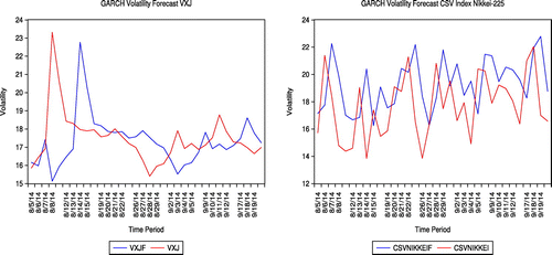
Figure 8. Volatility forecast of VXJ and cross-sectional volatility index (CSV) using EGARCH in the Japanese market.

5. Conclusion

In this paper, we proposed the CSV model to be applied in one of the Asian markets, namely the Japanese market. This is obtained by finding consistent estimations of parameters in financial market models using a single cross section of return data. The analysis of the relationship between the returns and the underlying assets and the volatility is aligned using the CSV and CBOE VIX index methodology. There are advantages in using a CSV method due to its model-free nature; also, this model may fit to any region, sector and style in the world equity market at any frequency. The model is also independent and there is no need to resort to any auxiliary option market. Generally, the systematic and average specific volatility indicators are highly correlated since both reflect the aggregate uncertainty encountered by investors, financial institutions and practitioners.

This paper suggests that the CSV is applicable in the Japanese market. To the best of our knowledge, this approach is the first to be examined in one of the Asian markets. A small number of Asian countries have an options markets that would allow for the classic VIX approach to construct the volatility index measurement. So, based on our results, the NIKKEI-225 CSV index is less volatile compared to the VXJ. The volatility index is dominantly low and consistent except during the uncertainty of the financial crisis. The main reason for constructing the CSV index is to allow the less derivative options market to measure the volatility index. It can be applied to markets that do not have an accompanying options component. We provide a statistical argument to support that an equally weighted measure of average idiosyncratic variance would forecast market return and show that this measure displays a sizable correlation with economic uncertainty. From the results gained, a high correlation exists between the VIX index and the CSV, possibly a model-free efficient and unbiased proxy for the specific risk in an Asian market. Ultimately, we wish to apply the CSV measure as a replacement for the VIX-styled measure to markets where the later is not practical. To validate this assertion, we demonstrated how the CSV measure and the VXJ measure are correlated. We have estimated measures of a cross-sectional rolling window of correlation in order to determine the pattern of correlation between the CBOE VIX and CSV index within a period of 252 days. The correlation moves in the same direction between the US market and Japanese market, although it may not be consistent over time due to factors including the changes in the financial market conditions. Our results demonstrate a statically significant positive conditional volatility estimate using the GARCH and E-GARCH models. It is found that the CSV approach is also a good predictor of the CBOE VIX model when estimating the idiosyncratic volatility. As a good volatility index model, the model should be able to forecast volatility (Engle & Patton, 2001).

Acknowledgements

For considerable improvements of the paper, we would like to thank the Editor, as well as anonymous referees.

Additional information

Funding

This work would not have been possible without the financial support of our government sponsorship, MARA.

Notes on contributors

Futeri Jazeilya Md Fadzil

Futeri Jazeilya Md Fadzil is a PhD candidate in Computational Finance of University of Essex, England particularly interests in modelling of financial markets and computational risk management. Currently, she is writing a thesis on volatility index for non-derivatives market in Asian. She has spoken at several conferences on the project that is currently accomplishing.

John G. O’Hara

John G. O’Hara whom is currently a senior lecturer at the Centre for Computational Finance and Economic Agents, University of Essex, England. He has over 30 years of teaching and research experience in mathematics and finance. He has published 36 articles many in leading journals. He is a reviewer for numerous journals, including Mathematical Reviews.

Wing Lon Ng

Wing Lon Ng is currently attached with Bounded Rationality Advancement in Computational Intelligence Laboratory (BRACIL). His general research interests are financial econometrics, time series analysis and stochastic point processes, microeconometrics, copula methods, advanced fast Fourier transforms, filtering techniques and duration, and survival analysis.

Notes

1 The fluctuation of asset prices may change at times along with the globalisation of the world economy. If the equity market is unstable, it will give a negative impact on economic growth, financial resources and income distribution. It may also lead to increased poverty.

2 The third proposition of the equally weighted CSV in idiosyncratic variance context, is proved to appear a consistent and asymptotically efficient estimator based on the study of Garcia et al. (2011).

3 Average idiosyncratic variance is an average measure as observed, which can be obtained by averaging across assets such as individual idiosyncratic variance estimates.

4 Daily stock return, stock price and shares outstanding data through this period are obtained from Datastream.

5 An old price of the asset that does not reflect the most recent information.

References

- Ahoniemi, K. (2006). Modeling and forecasting implied volatility- an econometric analysis of the vix index. Helsinki: HECER - Helsinki Center of Economic Research, University of Helsinki.
- Ang, A., Hodrick, R. J., Xing, Y., & Zhang, X. (2006). The cross-section of volatility and expected returns. The Journal of Finance, 61, 259–299.
- Ankrim, E. M., & Ding, Z. (2002). Cross-sectional volatility and return dispersion. Financial Analysts Journal, 58, 67–73.
- Bagchi, B. (2016). Volatility spillovers between exchange rates and indian stock markets in the post-recession period: an aparch approach. International Journal of Monetary Economics and Finance, 9, 225–244.
- Bentes, S. R. (2015). A comparative analysis of the predictive power of implied volatility indices and garch forecasted volatility. Physica A: Statistical Mechanics and its Applications, 424, 105–112.
- Brandt, M. W., & Jones, C. S. (2006). Volatility forecasting with range-based egarch models. Journal of Business & Economic Statistics, 24, 470–486.
- Campbell, J. Y., Lettau, M., Malkiel, B. G., & Xu, Y. (2001). Have individual stocks become more volatile? An empirical exploration of idiosyncratic risk. The Journal of Finance, 56(1), 1–43.
- Cutler, D. M., Katz, D. Q., Sheiner, L., & Wooldridge, J. (1989). Stock market volatility, cross-section volatility, and stock returns (Working Paper 1989). Cambridge: Massachusetts Institute of Technology.
- Engle, R. F., & Patton, A. J. (2001). What good is a volatility model. Quantitative Finance, 1, 237–245.
- Fukasawa, M., Ishida, I., Maghrebi, N., Oya, K., Ubukata, M., & Yamazaki, K. (2011). Model-free implied volatility: from surface to index. International Journal of Theoretical and Applied Finance, 14, 433–463.
- Garcia, R., Mantilla-Garcia, D., & Martellini, L. (2011). Idiosyncratic risk and the cross-section of stock returns (Working Paper, 5:57). Nice: EDHEC-Risk Institute.
- Garcia, R., Mantilla-Garcia, D., & Martellini, L. (2014). A model-free measure of aggregate idiosyncratic volatility and the prediction of market returns. Journal of Financial and Quantitative Analysis, 49, 1133–1165.
- Goltz, F., Guobenzaite, R., & Martellini, L. (2011). Introducing a new form of volatility index: The cross-sectional volatility index. Nice: EDHEC-Risk Institute.
- Hohensee, M., & Lee, K. (2006). A survey on hedging markets in Asia: a description of asian derivatives markets from a practical perspective. Asian Bond Markets: Issues and Prospects, BIS Papers, 30, 261–81.
- Kenmoe, S. R. N., & Tafou, C.D. (2014). The implied volatility analysis: The South African experience. arXiv preprint arXiv:1403.5965.
- Liu, H. C., Lee, Y. H., & Lee, M. C. (2009). Forecasting china stock markets volatility via garch models under skewed-ged distribution. Journal of Money, 7, 5–15.
- Merton, R. C. (1987). A simple model of capital market equilibrium with incomplete information. The Journal of Finance, 42, 483–510.
- Nartea, G. V., Ward, B. D., & Yao, L. J. (2011). Idiosyncratic volatility and cross-sectional stock returns in southeast asian stock markets. Accounting & Finance, 51, 1031–1054.
- Siriopoulos, C., & Fassas, A. (2012). An investor sentiment barometer greek implied volatility index. Global Finance Journal, 23, 77–93.
- Su, C. (2010). Application of egarch model to estimate financial volatility of daily returns: The empirical case of China (Master’s thesis). University of Gothenburg, Gothenburg.
- Whaley, R. E. (2000). The investor fear gauge. The Journal of Portfolio Management, 26, 12–17.
- Xu, Y., & Malkiel, B. G. (2004). Idiosyncratic risk and security returns. In AFA 2001 New Orleans Meetings.Dallas: The University of Texas.