Optimal execution strategy in liquidity framework

Abstract

A trader wishes to execute a given number of shares of an illiquid asset. Since the asset price also depends on the trading behaviour, the trader main aim is to find the execution strategy that minimizes the related expected costs. We solve this problem in a discrete time framework, by modeling the asset price dynamic as an arithmetic random walk with drift and volatility both modeled as Markov stochastic processes. The market impact is assumed to follow a Markov process. We found the unique execution strategy minimizing the implementation shortfall when short selling is allowed. This optimal strategy is given as solution of a forward-backward system of stochastic equations depending on conditional expectations of future values of model parameters. In the opposite case, namely when short selling is prohibited, we numerically obtain the solution for the associated Bellman equation that an optimal trading strategy must satisfy.

Keywords:

• pricing model
• liquid / illiquid market
• forward-backward stochastic differential equations
• Bellman equation
• optimal execution strategy

Public Interest Statement

We show the unique, analytical, execution strategy minimizing the implementation shortfall, when short selling is allowed, for a trader executing a given number of shares of an illiquid asset. We also numerically obtain the solution for the associated Bellman equation that an optimal trading strategy must satisfy when short selling is prohibited.

1. Introduction

The present work deals with the problem of optimally selling a fixed number of share of an asset in an illiquid economy. This means that the price process of the asset depends also on the trading strategy implemented by the trader. Therefore every transaction implies a change on the price, which is called market impact. Consequently, a large order may be split into more smaller orders to reduce the overall market impact. We assume that these smaller orders are finitely many so that the problem can be treated in a discrete-time framework. It follows that the main goal is to find the execution strategy, i.e. to choose the size of each individual order, which minimizes the related expected cost.

Optimal selling strategies in a liquidity framework have been studied in Almgren and Chriss (1999,   2001), where the so called Almgren-Chriss model is developed. In the Almgren-Chriss model the asset price process is modeled as a risk-neutral Arithmetic Random Walk (ARW) characterized by a constant volatility over all the liquidation interval. Moreover the market impact functions are linear in the sold quantities and the involved parameters are also assumed to be constants. In Almgren and Chriss (2001) optimal execution strategies are found explicitly by considering a minimization criterion based on a combination between the expectation and the variance of the cost, namely the mean-variance criterion.

In Cheridito and Sepin (2014) the authors extended the previous approach by modeling the volatility and the liquidity parameters by stochastic processes. When the objective is to minimize the expectation of the implementation cost the optimal solution is found explicitly. On the other hand, using the mean-variance criterion the optimal execution strategy cannot be stated explicitly, nevertheless the related Bellman equations are derived and then exploited to numerically obtain the associated optimal solutions by a discretization of the control space. It is worth to mention that such an approach could be in principle used also in rather different contexts as the ones related, e.g. to microbiological modelization, see, e.g. Barbu, Cordoni, and Di Persio (2016), or the abstract analysis of signals traveling through networks, see, e.g. Di Persio and Ziglio (2011), and references therein. Similar problems have been also studied, e.g. in Cetin and Rogers (2007), see also Ku, Lee, and Zhu (2012) and references therein, while in, e.g. Gokay, Roch, and Soner (2010) and Benazzoli and Di Persio (2014), related continuous time frameworks are also

In what follows we generalize previous results by removing the restriction of a zero drift term in the asset price dynamic. In particular we model the drift of the asset price process as a Markov chain. We would like to underline that, even if the obtained results are not surprising, our approach allows to treat a rather general setting. In particular, we get explicitly some of those further useful insights claimed by Almgren and Chriss (2001, Section 6).

Note that the optimal execution problem has been also studied in a continuous time setting. In Gatheral and Schied (2011), resp. in Brigo and Di Graziano (2014), explicit solutions have been provided under the assumption that the unaffected price process, that is the price process when the trader does not enter in the market, follows a Geometric Brownian Motion (GBM), resp. a displaced diffusion process. Moreover in Schied (2013) a robustness property for the optimal strategies is proved. Indeed, under a specified cost criterion, the form of the solution is independent on the unaffected price process, provided that it is a square integrable martingale.

We underline that similar problems have been studied, e.g. in Cetin and Rogers (2007), in Ku et al. (2012), see also references therein, as well as in Gokay et al. (2010) and Benazzoli and Di Persio (2014), where continuous time frameworks have been considered. The paper is organized as follows: in Section 2 we present the model; Section 3 is devoted to the computation of the trading solution that minimizes expected costs in a market where short-selling is allowed; while Section 4 addresses the same problem but in a market where short-selling is banned; finally, in Section 5, we provide the simulation results.

2. The model

A trader, who holds $X_0\in {\mathbb{R}}^{+}$ shares of an asset, wants to liquidate his entire position within a fixed deadline T. If the investor cannot sell (and buy) the asset continuously, then a discrete time model is obtained. The time interval $[0,T]$ is divided into N subintervals of the same length, denoted by $\mathit{\tau }:=\frac{T}{N}$ and, at every time step $t_{n-1}=(n-1)\mathit{\tau }$, with $n=1,\dots ,N$, the trader chooses the volume, i.e. the number of shares $y_n$, to sell in the succeeding subinterval $(t_{n-1},t_n]$. A trading list is the N-tuple of the sold quantities ${\{y_n\}}_{n=1}^N$, whereas an execution strategy is a $(N+1)$-tuple $(x_0,x_1,\dots ,x_N)$ where $x_n$ represents the volume of shares still held by the trader at time $t_n$. The execution strategy is strictly related to the related trading list, since $y_n=x_{n-1}-x_n$ and $x_n=X_0-{\sum }_{k=1}^n{y}_k={\sum }_{k=n+1}^N{y}_n$, and therefore by knowing the strategy x, the corresponding trading list $y^{(x)}$ is computable, and viceversa.

Since the asset is illiquid, when a treader acts in the market, this causes a direct variation of the price. Such a phenomenon is called market impact, being modeled by two parts, namely the temporary, resp. the permanent, component. The former refers to the price modification, in a given time interval, only due to the sale occurred in the immediately preceding time window, whereas the latter takes into account the price variation that persists throughout the remaining trading time.

The initial asset price is a known, fixed value $S_0$. Then the dynamic of the price follows the stochastic process ${\tilde{S}}_t$ defined by the equation(1) $$\begin{array}{c}\hfill {\tilde{S}}_n=S_{n-1}-{\mathit{\eta }}_n{y}_n,\end{array}$$(1)

where$$\begin{array}{c}\hfill S_n=S_{n-1}+{\mathit{\sigma }}_n\sqrt{\mathit{\tau }}{\mathit{\xi }}_n+{\mathit{\alpha }}_n\mathit{\tau }-c{y}_n.\end{array}$$

Due to the two different components of the market impact, the actual price ${\tilde{S}}_n$ is built in more steps. Consider the process ${\{{\overline{S}}_n\}}_n$ defined by ${\overline{S}}_n={\overline{S}}_{n-1}+{\mathit{\sigma }}_n\sqrt{\mathit{\tau }}{\mathit{\xi }}_n+{\mathit{\alpha }}_n\mathit{\tau }$. $\overline{S}$, called the unaffected price, represents the price per share of the asset which would occur in a impact-free market. Therefore the parameter c models the permanent market impact and it is assumed to be positive and constant over all the liquidation time $[0,T]$. Note that the asset price at time $t_n$, i.e. ${\tilde{S}}_n$, depends through the permanent component of the market impact c on all the previous sold quantities, namely on $y_1,\dots ,y_{n-1}$, summed up in $S_{n-1}$. On the other hand, ${\tilde{S}}_n$ depends on the temporary market impact, modeled by the stochastic process ${\{{\mathit{\eta }}_n\}}_n$ only through the shares sold at time $t_n$, namely $y_n$. The stochastic processes ${\{{\mathit{\alpha }}_n\}}_n$ and ${\{{\mathit{\sigma }}_n\}}_n$ represent the drift process, resp. the volatility process, of the asset. Furthermore the process ${\{{\mathit{\xi }}_n\}}_n$ is a sequence of independent standard normal random variables, i.e. ${\mathit{\xi }}_n\sim N(0,1)$, $\forall n\in \left\{0,\dots ,N\right\}$.

In what follows, we assume that the random variables $S_n$, ${\mathit{\alpha }}_n$, ${\mathit{\sigma }}_n$ and ${\mathit{\eta }}_n$ are observable at time $t_n$, and moreover, being ${\mathcal{F}}_n$ the filtration $\mathit{\sigma }(S_i,{\mathit{\alpha }}_i,{\mathit{\sigma }}_i,{\mathit{\eta }}_i:0\le i\le n)$, ${\mathit{\xi }}_n$ is assumed to be independent of the $\mathit{\sigma }$-algebra $\mathit{\sigma }({\mathcal{F}}_{n-1},{\mathit{\alpha }}_n,{\mathit{\sigma }}_n,{\mathit{\eta }}_n)$. We assume that $({\mathit{\alpha }}_n,{\mathit{\sigma }}_n,{\mathit{\eta }}_n)$ can take finitely many values in $\mathbb{R}\times {\mathbb{R}}_{+}^2$, and we set$$\begin{array}{c}\hfill \mathbb{P}\left[({\mathit{\alpha }}_n,{\mathit{\sigma }}_n,{\mathit{\eta }}_n)=w|{\mathcal{F}}_{n-1}\right]=\mathbb{P}\left[({\mathit{\alpha }}_n,{\mathit{\sigma }}_n,{\mathit{\eta }}_n)=w|({\mathit{\alpha }}_{n-1},{\mathit{\sigma }}_{n-1},{\mathit{\eta }}_{n-1})=v\right]=:p_{n-1}^{vw}.\end{array}$$

Hence, ${({\mathit{\alpha }}_n,{\mathit{\sigma }}_n,{\mathit{\eta }}_n)}_n$ is a Markov chain with finite state space V, and $p_{n-1}^{vw}$ denotes the related transition probability. In order to simplify the notation, we shall indicate by ${\mathbb{E}}_n^v[·]$ the expectation computed at time $t_n$ knowing that $({\mathit{\alpha }}_n,{\mathit{\sigma }}_n,{\mathit{\eta }}_n)=v$. We assume that ${\mathbb{E}}_{n-1}^v[{\tilde{\mathit{\eta }}}_n]>0$ for all $v\in V$ and $n\ge 1$, so that, on average, a sale of the asset lowers the asset price down while a buying raises it.

In this setting, an execution strategy x is admissible if it satisfies the following conditions:

(1)	${\{x_n\}}_{n=0}^N$ is predictable with respect to ${\{{\mathcal{F}}_n\}}_{n=0}^N$ ;
(2)	$x_0=X_0$ and $x_N=0$.

  Condition $x_N=0$ is crucial for the problem we are interest in, since it guarantees that the asset has been completely liquidated within the deadline T. The set of all admissible strategies is denote by $\mathcal{A}$. Note that we do not request that admissible strategies have to fulfill the pure selling property, hence the trader is allowed to short sell the asset to lower the implementation shortfall. For an admissible strategy $x\in \mathcal{A}$, the implementation shortfall C(x) is defined as the difference between the market value of the initial position and the total gain, namely$$\begin{array}{cc}\hfill C(x)& =X_0{S}_0-\sum _{n=1}^N{y}_n{\tilde{S}}_n\hfill \\ \hfill & =\frac{c}{2}{X}_0^2+\sum _{n=1}^N\left[{\tilde{\mathit{\eta }}}_n{(x_{n-1}-x_n)}^2-({\mathit{\sigma }}_n\sqrt{\mathit{\tau }}{\mathit{\xi }}_n+{\mathit{\alpha }}_n\mathit{\tau })x_n\right]\hfill \end{array}$$

where ${\tilde{\mathit{\eta }}}_n={\mathit{\eta }}_n-\frac{c}{2}$. It provides the ex-post transaction cost of the strategy.

3. Optimal execution strategy

In our setting, the trader seeks the strategy that minimizes the expectation of the implementation shortfall over all admissible strategies $\mathcal{A}$, that is $x^{\ast }=arg{min}_{x\in \mathcal{A}}{\mathbb{E}}_0^v[C(x)]$. The following theorem provides a complete answer to this question.

Theorem 3.1

The minimum of the expected implementation shortfall is given by$$\begin{array}{c}\hfill \underset{x\in \mathcal{A}}{min}{\mathbb{E}}_0^v[C(x)]=\left(a_0^v+\frac{c}{2}\right)X_0^2-b_0^v{X}_0+c_0^v,\end{array}$$

where the coefficients $a_n^v$, $b_n^v$ and $c_n^v$ are computed by the backwards recursion$$\begin{array}{c}\hfill a_{N-1}^v={\mathbb{E}}_{N-1}^v[{\tilde{\mathit{\eta }}}_N],b_{N-1}^v=c_{N-1}^v=0,\end{array}$$

and$$\begin{array}{cc}\hfill a_{n-1}^v& =\frac{{\mathbb{E}}_{n-1}^v[{\tilde{\mathit{\eta }}}_n]{\sum }_{w\in V}{p}_{n-1}^{vw}{a}_n^w}{{\mathbb{E}}_{n-1}^v[{\tilde{\mathit{\eta }}}_n]+{\sum }_{w\in V}{p}_{n-1}^{vw}{a}_n^w}\hfill \\ \hfill b_{n-1}^v& =\frac{{\mathbb{E}}_{n-1}^v[{\tilde{\mathit{\eta }}}_n]({\mathbb{E}}_{n-1}^v[{\mathit{\alpha }}_n]\mathit{\tau }+{\sum }_{w\in V}{p}_{n-1}^{vw}{b}_n^w)}{{\mathbb{E}}_{n-1}^v[{\tilde{\mathit{\eta }}}_n]+{\sum }_{w\in V}{p}_{n-1}^{vw}{a}_n^w}\hfill \\ \hfill c_{n-1}^v& =-\frac{{\left({\mathbb{E}}_{n-1}^v[{\mathit{\alpha }}_n]\mathit{\tau }+{\sum }_{w\in V}{p}^{vw}{b}_n^w\right)}^2}{4({\mathbb{E}}_{n-1}^v[{\tilde{\mathit{\eta }}}_n]+{\sum }_{w\in V}{p}_{n-1}^{vw}{a}_n^w)}+\sum _{w\in V}{p}^{vw}{c}_n^w\hfill \end{array}$$

for $n<N-1$. The unique optimal execution strategy that realizes such a minimum is recursively given by$$\begin{array}{cc}\hfill x_n{|}_{x_{n-1},({\mathit{\alpha }}_{n-1},{\mathit{\sigma }}_{n-1},{\mathit{\eta }}_{n-1})}& =\frac{{\mathbb{E}}_{n-1}^v[{\tilde{\mathit{\eta }}}_n]}{{\mathbb{E}}_{n-1}^v[{\tilde{\mathit{\eta }}}_n]+{\sum }_{w\in V}{p}_{n-1}^{vw}{a}_n^w}{x}_{n-1}\hfill \\ \hfill & +\frac{{\mathbb{E}}_{n-1}^v[{\mathit{\alpha }}_n]\mathit{\tau }+{\sum }_{w\in V}{p}_{n-1}^{vw}{b}_n^w}{2\left({\mathbb{E}}_{n-1}^v[{\tilde{\mathit{\eta }}}_n]+{\sum }_{w\in V}{p}_{n-1}^{vw}{a}_n^w\right)}\hfill \end{array}$$

for all $n=1,\dots ,N-1$.

Similarly as in Almgren and Chriss (2001), the trajectory is the sum of two distinct terms: the first one depending only on the process ${\{{\mathit{\eta }}_n\}}_n$ and the number of shares held by the trader, and the second one which takes into account ${\{{\mathit{\eta }}_n\}}_n$ and the processes ${\{{\mathit{\alpha }}_n\}}_n$ and ${\{{\mathit{\sigma }}_n\}}_n$, hence it is independent on the portfolio’s volume.

Proof

Let ${\mathcal{A}}_n(z)$ be the set of all predictable strategies ${\{x_k\}}_{k=n}^N$ such that $x_n=z$ and $x_N=0$, and define the functional $J_n^v(z):={min}_{x\in {\mathcal{A}}_n(z)}{\mathbb{E}}_n^v[Q_n(x)]$, where$$\begin{array}{c}\hfill Q_n(x):=\sum _{k=n+1}^N\left[{\tilde{\mathit{\eta }}}_k{(x_{k-1}-x_k)}^2-({\mathit{\sigma }}_k\sqrt{\mathit{\tau }}{\mathit{\xi }}_k+{\mathit{\alpha }}_k\mathit{\tau })x_k\right].\end{array}$$

Moreover, we have that$$\begin{array}{c}\hfill {\mathbb{E}}_n^v[Q_n(x)]={\mathbb{E}}_n^v\left[\sum _{k=n+1}^N\left[{\tilde{\mathit{\eta }}}_k{(x_{k-1}-x_k)}^2-{\mathit{\alpha }}_k\mathit{\tau }{x}_k\right]\right]\end{array}$$

since, by previous assumptions, each ${\mathit{\xi }}_k$, with $k>n$, is independent on the $\mathit{\sigma }$-algebra $\mathit{\sigma }({\mathcal{F}}_{n-1},{\mathit{\alpha }}_n,{\mathit{\sigma }}_n,{\mathit{\eta }}_n)$ and it is normally distributed with mean 0. In what follows we show, by backward induction on n, that, for each $n\le N-1$, it holds$$\begin{array}{c}\hfill J_n^v(x_n)=a_n^v{x}_n^2-b_n^v{x}_n+c_n^v,(P)\end{array}$$

where $a_n^v$, $b_n^v$ and $c_n^v$ are as in Theorem 3.1. For $n=N-1$, property (P) follows immediately since by the definitions of Q and J $$\begin{array}{cc}\hfill J_{N-1}^v(x_{N-1})& ={\mathbb{E}}_{N-1}^v[{\tilde{\mathit{\eta }}}_N]{(x_{N-1}-x_N)}^2\hfill \\ \hfill & ={\mathbb{E}}_{N-1}^v[{\tilde{\mathit{\eta }}}_N]{(x_{N-1})}^2.\hfill \end{array}$$

Assuming that the claim (P) holds for $n>1$,(2) $$\begin{array}{cc}\hfill J_{n-1}^v(x_{n-1})& =\underset{x\in {\mathcal{A}}_{n-1}(x_{n-1})}{min}{\mathbb{E}}_{n-1}^v[Q_n(x)]\hfill \\ \hfill & =\underset{x\in {\mathcal{A}}_{n-1}(x_{n-1})}{min}{\mathbb{E}}_{n-1}^v[{\tilde{\mathit{\eta }}}_n]{(x_{n-1}-x_n)}^2-{\mathbb{E}}_{n-1}^v[{\mathit{\alpha }}_n]\mathit{\tau }{x}_n+{\mathbb{E}}_{n-1}^v[Q_{n+1}(x)]\hfill \\ \hfill & =\underset{x_n}{min}{\mathbb{E}}_{n-1}^v[{\tilde{\mathit{\eta }}}_n]{(x_{n-1}-x_n)}^2-{\mathbb{E}}_{n-1}^v[{\mathit{\alpha }}_n]\mathit{\tau }{x}_n+\sum _{w\in V}{p}_{n-1}^{vw}{J}^w(x_n)\hfill \\ \hfill & =\underset{x_n}{min}{\mathbb{E}}_{n-1}^v[{\tilde{\mathit{\eta }}}_n]{(x_{n-1}-x_n)}^2-{\mathbb{E}}_{n-1}^v[{\mathit{\alpha }}_n]\mathit{\tau }{x}_n+\sum _{w\in V}{p}_{n-1}^{vw}(a_n^w{x}_n^2-b_n^w{x}_n+c_n^w),\hfill \end{array}$$(2)

where the function to minimize is strictly convex; hence there exists a unique minimum which can be found solving the first order condition, i.e.(3) $$\begin{array}{c}\hfill -2{\mathbb{E}}_{n-1}^v[{\tilde{\mathit{\eta }}}_n](x_{n-1}-x_n)-{\mathbb{E}}_{n-1}^v[{\mathit{\alpha }}_n]\mathit{\tau }+\sum _{w\in V}{p}_{n-1}^{vw}(2a_n^w{x}_n-b_n^w)=0.\end{array}$$(3)

Therefore the minimum is given by(4) $$\begin{array}{c}\hfill x_n^{\ast }=\frac{{\mathbb{E}}_{n-1}^v[{\tilde{\mathit{\eta }}}_n]}{{\mathbb{E}}_{n-1}^v[{\tilde{\mathit{\eta }}}_n]+{\sum }_{w\in V}{p}_{n-1}^{vw}{a}_n^w}{x}_{n-1}+\frac{{\mathbb{E}}_{n-1}^v[{\mathit{\alpha }}_n]\mathit{\tau }+{\sum }_{w\in V}{p}_{n-1}^{vw}{b}_n^w}{2\left({\mathbb{E}}_{n-1}^v[{\tilde{\mathit{\eta }}}_n]+{\sum }_{w\in V}{p}_{n-1}^{vw}{a}_n^w\right)}.\end{array}$$(4)

Equation (4) gives the optimal quantity to hold at time $t_n$ knowing the quantity held at the previous time, $t_{n-1}$, so that $x^{\ast }=(X_0,x_1^{\ast },\dots ,x_{N-1}^{\ast },0)$ is the optimal execution strategy as stated in the Theorem and, replacing $x_n$ by (4) in Equation (2), we have$$\begin{array}{cc}\hfill J_{n-1}^v(x_{n-1})& =\frac{{\mathbb{E}}_{n-1}^v[{\tilde{\mathit{\eta }}}_n]{\sum }_{w\in V}{p}_{n-1}^{vw}{a}_n^w}{{\mathbb{E}}_{n-1}^v[{\tilde{\mathit{\eta }}}_n]+{\sum }_{w\in V}{p}_{n-1}^{vw}{a}_n^w}{(x_{n-1})}^2\hfill \\ \hfill & -\frac{{\mathbb{E}}_{n-1}^v[{\tilde{\mathit{\eta }}}_n]\left({\mathbb{E}}_{n-1}^v[{\mathit{\alpha }}_n]\mathit{\tau }+{\sum }_{w\in V}{p}_{n-1}^{vw}{b}_n^w\right)}{{\mathbb{E}}_{n-1}^v[{\tilde{\mathit{\eta }}}_n]+{\sum }_{w\in V}{p}_{n-1}^{vw}{a}_n^w}{x}_{n-1}\hfill \\ \hfill & -\frac{{\left({\mathbb{E}}_{n-1}^v[{\mathit{\alpha }}_n]\mathit{\tau }+{\sum }_{w\in V}{p}_{n-1}^{vw}{b}_n^w\right)}^2}{4\left({\mathbb{E}}_{n-1}^v[{\tilde{\mathit{\eta }}}_n]+{\sum }_{w\in V}{p}_{n-1}^{vw}{a}_n^w\right)}+\sum _{w\in V}{p}_{n-1}^{vw}{c}_n^w,\hfill \end{array}$$

that implies (P) for $n-1$, concluding the proof. $\square$

Remark 1

In the case of constant parameters, i.e. ${\mathit{\alpha }}_n\equiv \mathit{\alpha }$, ${\mathit{\sigma }}_n\equiv \mathit{\sigma }$ and ${\mathit{\eta }}_n\equiv \mathit{\eta }$, the problem under consideration becomes$$\begin{array}{c}\hfill \underset{x\in \mathcal{A}}{min}{\mathbb{E}}_0^v[C(x)]=\underset{x\in \mathcal{A}}{min}\sum _{n=1}^N\tilde{\mathit{\eta }}{(x_{n-1}-x_n)}^2-\mathit{\alpha }\mathit{\tau }{x}_n,\end{array}$$

where $\tilde{\mathit{\eta }}=\mathit{\eta }-\frac{c}{2}$. Since the function we want to minimize is a strictly convex quadratic function in the control parameter $x_1,\dots ,x_{N-1}$, its unique minimum can be found by solving the following equations$$\begin{array}{c}\hfill -2\tilde{\mathit{\eta }}(x_{n-1}-x_n)+2\tilde{\mathit{\eta }}(x_n-x_{n+1})-\mathit{\alpha }\mathit{\tau }=0,\end{array}$$

for $n=1,\dots ,N-1$, whose solutions are given by$$\begin{array}{c}\hfill x_n=x(t_n)=\frac{\mathit{\alpha }}{4\mathit{\tau }\tilde{\mathit{\eta }}}{(t_n)}^2+b(t_n)+c,\end{array}$$b and c being constant parameters that can be estimated by using the boundary constraints $x_0=X_0$ and $x_N=0$. Therefore the unique optimal solution is(5) $$\begin{array}{c}\hfill x^{\ast }(t_k)=\left(\frac{X_0}{T}+\frac{\mathit{\alpha }}{4\tilde{\mathit{\eta }}}{t}_k\right)(T-t_k).\end{array}$$(5)

If the asset price process has no drift, i.e. $\mathit{\alpha }\equiv 0$, the optimal strategy reads as $x^{\ast }(t_k)=X_0-X_0\frac{t_k}{T}$. The latter is called the naive strategy, since the trader sells the same amount of shares at every time step $t_k$, namely the adopted strategy is simply linear in time. Note that the naive strategy does not depend neither on the market impact $\mathit{\eta }$, nor on the volatility $\mathit{\sigma }$, nor on the frequency of selling N.

Remark 2

It is interesting to observe that in the case of zero-drift, namely in the setting considered in Cheridito and Sepin (2014), the coefficients $b_k^v$ and $c_k^v$ are all zero and then the optimal solution reduces to(6) $$\begin{array}{c}\hfill x_n^{\ast }{|}_{x_{n-1},({\mathit{\alpha }}_{n-1},{\mathit{\sigma }}_{n-1},{\mathit{\eta }}_{n-1})}=\frac{{\mathbb{E}}_{n-1}^v[{\tilde{\mathit{\eta }}}_n]}{{\mathbb{E}}_{n-1}^v[{\tilde{\mathit{\eta }}}_n]+{\sum }_{w\in V}{p}_{n-1}^{vw}{a}_n^w}{x}_{n-1},\end{array}$$(6)

where the coefficients $a_k^v$ are defined as in Theorem 3.1. Note that if we assume zero drift, then the amount of shares sold in each interval time may vary depending on the expected future parameters, contrary to the constant parameters case, as seen in Remark 1.

4. Pure sell strategies

In this section the problem considered in Section 3 will be studied when the admissible set is reduced to only the pure sell strategies. In this frame, an admissible strategy is a $(N+1)$-tuple $x={\{x_n\}}_{n=0}^N$ such that:

• $x_0=X_0$ and $X_N=0$;

• $x_{n-1}\ge x_n$;

• ${\{x_n\}}_{n=0}^N$ is predicable with respect to ${\{{\mathcal{F}}_n\}}_{n=0}^N$.

In this scenario, short selling is not allowed since, for each n, $x_n\ge X_N=0$, i.e. $x_n$ is positive, and our purpose is to find the strategy that solves(7) $$\begin{array}{c}\hfill x^{\ast }=arg\underset{x\in {\mathcal{A}}^{\prime }}{min}{\mathbb{E}}_0^v[C(x)],\end{array}$$(7)

where ${\mathcal{A}}^{\prime }$ denotes the new admissible strategies set. Let J be the functional defined as before, but this time with respect to ${\mathcal{A}}^{\prime }$, then the following holds true.

Theorem 4.1

The functional J satisfies the Bellman equations(8) $$\begin{array}{c}\hfill J_{N-1}^v(x_{N-1})={\mathbb{E}}_{N-1}^v[{\tilde{\mathit{\eta }}}_n]x_{N-1}^2,\end{array}$$(8)

and(9) $$\begin{array}{cc}\hfill J_{n-1}^v(x_{n-1})& =\underset{x_n\in [0,x_{n-1}]}{min}\left[{\mathbb{E}}_{n-1}^v[{\tilde{\mathit{\eta }}}_n]{(x_{n-1}-x_n)}^2\right.\hfill \\ \hfill & \left.-{\mathbb{E}}_n^v[{\mathit{\alpha }}_n]\mathit{\tau }{x}_n+\sum _{w\in V}{p}_{n-1}^{vw}{J}_n^w(x_n)\right],\hfill \end{array}$$(9)

for all $n\le N-1$. Moreover there exists a unique strategy $x\in {\mathcal{A}}^{\prime }$ that solves (8)–(9) given by the solution of the minimizing problem (7).

Proof

Taking $n=N-1$ we have $J_{N-1}^v(x_{N-1})={\mathbb{E}}_{N-1}^v[{\tilde{\mathit{\eta }}}_N]{(x_{N-1}-x_N)}^2={\mathbb{E}}_{N-1}^v[{\tilde{\mathit{\eta }}}_N]{(x_{N-1})}^2,$ while, for $n\le N-1$ we obtain$$\begin{array}{cc}\hfill J_{n-1}^v& =\underset{x\in {\mathcal{A}}_{n-1}(x_{n-1})}{min}{\mathbb{E}}_{n-1}^v[Q_n(x)]\hfill \\ \hfill & =\underset{x\in {\mathcal{A}}_{n-1}(x_{n-1})}{min}{\mathbb{E}}_{n-1}^v[{\tilde{\mathit{\eta }}}_n]{(x_{n-1}-x_n)}^2-{\mathbb{E}}_{n-1}^v[{\mathit{\alpha }}_n]\mathit{\tau }{x}_n+{\mathbb{E}}_{n-1}^v[Q_{n+1}(x)]\hfill \\ \hfill & =\underset{x_n\in [0,x_{n-1}]}{min}{\mathbb{E}}_{n-1}^v[{\tilde{\mathit{\eta }}}_n]{(x_{n-1}-x_n)}^2-{\mathbb{E}}_{n-1}^v[{\mathit{\alpha }}_n]\mathit{\tau }{x}_n+\sum _{w\in V}{p}_{n-1}^{vw}{J}^w(x_n),\hfill \end{array}$$

and, since the function to be minimized is strictly convex due to the assumption ${\mathbb{E}}_{n-1}^v[{\tilde{\mathit{\eta }}}_n]>0$, there exists a unique solution (optimal strategy) $x^{\ast }$ to (7). $\square$

Remark 3

Notice that if the asset price process has zero drift the optimal execution strategy found in the previous case, i.e. (6), is already of pure sell.

5. Simulations

In what follows we shall present different simulations related to the results obtained in previous sections. In particular some explicit numerical examples for the behaviour of the trader in a market with liquidity risks in different economic scenarios are provided. The values chosen for the model parameters are as in Table 1.

Table 1. Parametres value

Parameter	Symbol	Value
Initial asset price	$S_0$	172 $ /share
Initial asset position	$X_0$	35,000 share
Liquidation time	T	100 min
Number of subintervals	N	100
Permanent impact	c	$2.5\times {10}^{-7}$
Temoprary impact	${\mathit{\eta }}_{\text{low}}$	$1\times {10}^{-6}$
	${\mathit{\eta }}_{\text{med}}$	$5\times {10}^{-6}$
	${\mathit{\eta }}_{\text{high}}$	$25\times {10}^{-6}$
Volatility state	${\mathit{\sigma }}_{\text{low}}$	$3.51\times {10}^{-3}$
	${\mathit{\sigma }}_{\text{med}}$	$3.33\times {10}^{-2}$
	${\mathit{\sigma }}_{\text{high}}$	$1.172\times {10}^{-1}$
Positive drift state	${\mathit{\alpha }}_{\text{low}}$	$2.2\times {10}^{-4}$
	${\mathit{\alpha }}_{\text{med}}$	$0.3\times {10}^{-3}$
	${\mathit{\alpha }}_{\text{high}}$	$0.8\times {10}^{-3}$
Negative drift state	${\mathit{\alpha }}_{\text{low}}$	$-4.2\times {10}^{-4}$
	${\mathit{\alpha }}_{\text{med}}$	$-1.8\times {10}^{-4}$
	${\mathit{\alpha }}_{\text{high}}$	$-8.3\times {10}^{-5}$

Throughout this section, the following assumptions will be in place. The processes ${\{{\mathit{\alpha }}_n\}}_n$, ${\{{\mathit{\sigma }}_n\}}_n$, ${\{{\mathit{\eta }}_n\}}_n$ and ${\{{\mathit{\xi }}_n\}}_n$ evolve independently of each other and the first three are time-homogeneous Markov chains with three state space, resp. low, med and high. Therefore the transition probability matrices denoted by $p^{\mathit{\alpha }}$, $p^{\mathit{\sigma }}$ and $p^{\mathit{\eta }}$ do not depend on time, and, indeed, in our numeric implementation they read as follows:$$\begin{array}{cc}& p^{\mathit{\alpha }}=\left[\begin{array}{ccc}0.62& 0.18& 0.20\\ 0.30& 0.57& 0.13\\ 0.21& 0.19& 0.60\end{array}\right]p^{\mathit{\sigma }}=\left[\begin{array}{ccc}0.9349& 0.0434& 0.0217\\ 0.7164& 0.2239& 0.0597\\ 0.4400& 0.4800& 0.0800\end{array}\right]\hfill \\ \hfill & \text{and}{p}^{\mathit{\eta }}=\left[\begin{array}{ccc}0.50& 0.30& 0.20\\ 0.15& 0.80& 0.05\\ 0.05& 0.05& 0.90\end{array}\right].\hfill \end{array}$$

The trading time interval is set to be equal to 100 min and the asset can be traded every minute, i.e. the trader cannot split his sale into more than 100 trades.

We first consider a scenario where the trader believes that the asset price is likely to rise, namely the drift process is positive. The initial state of the parameters’ processes is equal to $({\mathit{\alpha }}_{\text{med}},{\mathit{\sigma }}_{\text{med}},{\mathit{\eta }}_{}\text{med})$. Theorem 3.1 states that, by following the optimal execution strategy, the expected cost equals $\mathbb{E}[C(x)]=-750.9407\mathrm{\$}$.

We simulate 50.000 possible paths of ${\{({\mathit{\alpha }}_n,{\mathit{\sigma }}_n,{\mathit{\eta }}_n,{\mathit{\xi }}_n)\}}_n$ and the related optimal strategies. In Figure 1(a) there are shown the average value of the optimal strategies (on the left side) and the corresponding standard deviation (on the right side), while Figure 1(b) shows the realizations of the implementation cost, with average cost of the simulated strategies equal to $-792.2788\mathrm{\$}$.

Figure 1. (a) Average and standard deviation of the optimal trading strategies with parameters given by Table 1 when the drift process is positive, and (b) Histogram of the implementation cost for the optimal trading strategies.

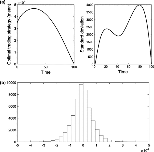
We would like to underline that in the previous case the expected and the average cost are negative, which means that the trader may take advantage from the fact that the price is likely to rise and make a positive gain. In particular Figure 1(a) shows that at first the trader actually buys other shares with the intention of reselling them later at a higher price.

In what follows we shall consider the optimal execution strategy problem when the price is likely to decrease, hence the drift parameters are negative, and we assume that short selling is allowed. As before, we assume that the Markov chain ${\{({\mathit{\alpha }}_n,{\mathit{\sigma }}_n,{\mathit{\eta }}_n)\}}_n$ starts from $({\mathit{\alpha }}_{}\text{med},{\mathit{\sigma }}_{}\text{med},{\mathit{\eta }}_{}\text{med})$. Figure 2(a) shows the average value of the optimal strategies (on the left side) and the corresponding standard deviation (on the right side) when 50.000 possible paths are simulated. Note that for this choice of parameters, the average strategy achieves negative values, therefore the trader actually short sells the asset. The corresponding costs are shown in the histogram of Figure 2(b). The expect cost is $\mathbb{E}[C(x)]=530.5309\mathrm{\$}$ while the average cost over the 50,000 simulations is $523.0289\mathrm{\$}$.

Figure 2. (a) Average and standard deviation of the optimal trading strategies with parameters given by Table 1 when the drift process is negative and short selling is allowed and (b) Histogram of the implementation cost for the optimal trading strategies.

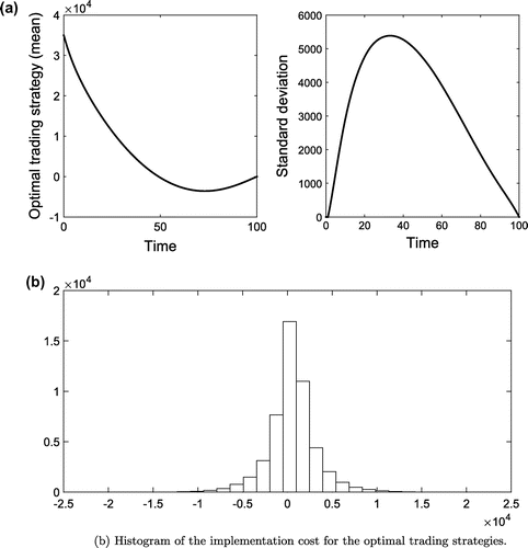
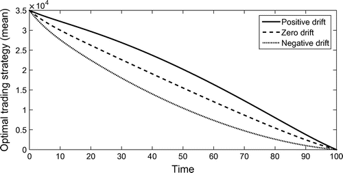
Figure 3 shows how the optimal execution strategy depends on the drift parameter. In the positive drift case we consider the following states$$({\mathit{\alpha }}_{\text{low}},{\mathit{\alpha }}_{\text{med}},{\mathit{\alpha }}_{\text{high}})=(0.42,0.8,1.1)\times {10}^{-4}$$

while for in the negative drift case we assume$$({\mathit{\alpha }}_{\text{low}},{\mathit{\alpha }}_{\text{med}},{\mathit{\alpha }}_{\text{high}})=-(1.2,0.8,0.23)\times {10}^{-4}.$$

As shown by the provided graphs, the drift determines the rate of selling, in particular we have that the financial player tends to sell slower in case of positive drift, being faster if we assume a negative drift. As a consequence, if the average drift is great enough, then the trader buys more shares of the asset even if his main goal is to liquidate them.

Figure 3. Comparison between optimal trading strategies for different drift values.

Figure 4. Comparison between optimal trading strategies when short selling is allowed and when it is denied.

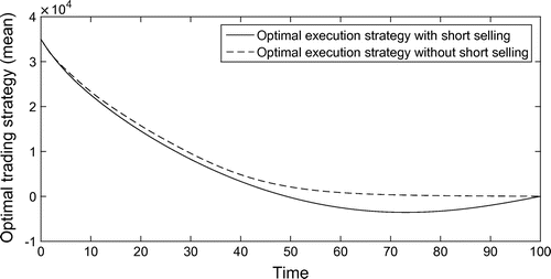
Table 2. Sensitivity and run-time performance

Simulation	Effective cost [$]	Absolute error [$]	Percent error	Execution time [s]
Positive drift case
10,000	$-823.2395$	72.2888	0.0963	39.2656
25,000	$-689.8894$	61.0514	0.0813	97.0904
50,000	$-714.0665$	36.8742	0.0491	195.8398
100,000	$-741.1059$	9.8348	0.0131	388.8039
200,000	$-747.2075$	3.7332	0.0050	779.3230
Negative drift case
10,000	519.2613	11.2696	0.0212	39.4368
25,000	540.1277	9.5309	0.0181	97.9121
50,000	523.0289	7.5020	0.141	194.0890
100,000	524.0302	6.5007	0.0123	390.6021
200,000	533.5788	3.0408	0.0057	774.7577

The accuracy of the proposed model can be studied by analysing the behaviour of the errors with respect to the number of simulations, the results are shown in Table 2. Notice that 50,000 simulations are enough to reduce the relative error in both cases below 5% and with 100,000 simulations both these errors are less than 1.5%. Obviously such an increment in the accuracy has to be payed in terms of increasing execution time, which grows linearly with the number of simulations. The latter is due to the fact that the majority of the algorithm’s running time is spent simulating the Markov chain ${\{({\mathit{\alpha }}_n,{\mathit{\sigma }}_n,{\mathit{\eta }}_n,{\mathit{\xi }}_n)\}}_n$.

Remark 4

We would like to underline that both the absolute and the percentage error show the same behaviour with respect to different values for the parameters $\mathit{\alpha }$, $\mathit{\sigma }$ and $\mathit{\eta }$. In particular, they decrease if we increase the number of simulations, paying the price of higher executions times. Concerning the time-step, when the liquidation deadline T is fixed, the execution time increases as N increases, namely as the length $\mathit{\tau }$ between two subsequent trades is shortened. Indeed we have to simulate more states for the related Markov chain ${\{({\mathit{\alpha }}_n,{\mathit{\sigma }}_n,{\mathit{\eta }}_n,{\mathit{\xi }}_n)\}}_n$, and also more values for the optimal executions strategy.

In order to have a direct comparison between the optimal trading strategies obtained when short selling is allowed and when not, we simultaneously report in Figure 4 the results related to those two different settings. When short selling is allowed the trader is more aggressive, this means he sells faster, and with the chosen parameters the optimal strategy reaches negative values. The average cost when short selling is allowed equals $538.0753\mathrm{\$}$, while when the trading strategy is forced to be positive, the average cost is grater, indeed it equals $558.5057\mathrm{\$}$.

The latter result is not surprising, since in the second case we add a condition for a strategy to be admissible, hence we are reducing the set from which the trader can choose the strategy to follow. A different reason which causes a higher average cost when short selling is forbidden is of computational type. Indeed by numerically solving the Bellman equation in Theorem 4.4, we discretize the position state $[0,X_0]$, therefore adding a further constraint for admissible trading strategies. In the previous case, we allowed the trader to sell in lots of 350 shares, that is the one percent of his initial position. How this constraint affects the optimal trading strategy can be better seen when the drift parameters are nearly zero, e.g. ${\mathit{\alpha }}_{\text{low}}=-9.2\times {10}^{-5},{\mathit{\alpha }}_{\text{med}}=-7.8\times {10}^{-5}$ and ${\mathit{\alpha }}_{\text{high}}=-8.3\times {10}^{-6}$, that is the case when although it is possible to sell short, the trader rarely uses such a strategy, so that the discrepancy between the two different strategies and their respective average costs is mostly due to the discretization.

Figure 5. Comparison between optimal trading strategies when short selling is allowed and when it is denied with different discretization size.

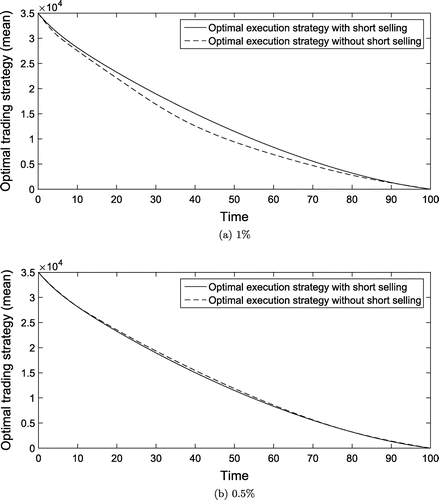
In the first case, i.e. Figure 5(a), when shortselling is forbidden the trader is allowed to sell in lots of one percent of his initial position (350 shares), while in the second one, i.e. Figure 5(b), in lots of 0.5 percent of his initial position (175 shares). In this second case the two optimal strategies are very similar, and so are the average costs which equal $348.6095\mathrm{\$}$, resp. $351.2562\mathrm{\$}$ when short selling is allowed, resp. when it is not. Instead, in the first case, the gap between the two average costs is greater, in fact the average costs equal $370.9495\mathrm{\$}$, resp. $393.3549\mathrm{\$}$.

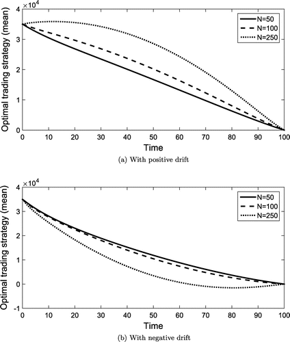
Last, but not least, we study how the optimal strategy depends on the parameter N in order to better understand the role of the time discretization. Since N represents the maximum number of trades in which a sale can be divided, then the trader can sell his asset with a higher frequency as N increases. Figure 6(a) and (b) show the optimal execution strategy for three different value of N, namely taking $N=50,100,200$, when the drift equals $({\mathit{\alpha }}_{\text{low}},{\mathit{\alpha }}_{\text{med}},{\mathit{\alpha }}_{\text{high}})=(0.42,0.8,1.1)\times {10}^{-4}$, resp. it equals $({\mathit{\alpha }}_{\text{low}},{\mathit{\alpha }}_{\text{med}},{\mathit{\alpha }}_{\text{high}})=-(1.2,0.8,0.23)\times {10}^{-4}$. The average costs, which have been computed running 50,000 simulations, are $291.9287\mathrm{\$}$, $119.5949\mathrm{\$}$, and $78.6512\mathrm{\$}$ for $N=50$, resp. $N=100$, resp. $N=200$, for the first choice of the drift, while they equal $500.4851\mathrm{\$}$ for $N=50$, resp. $382.6879\mathrm{\$}$ for $N=100$, resp. $297.4120)\mathrm{\$}$ for $N=200$in the second case. Such an analysis allows us to conclude that the execution cost decreases as N increases.

Figure 6. Comparison between optimal trading strategies with different time discretization size.

The latter result is mainly due to the fact that higher values of N imply a larger set of degrees of freedom, since the trader can buy/sell more often, or he can decide to stay out of the market. Figure 6 shows that when the investor can frequently trade in the market, i.e. $N=200$, is more aggressive. In the first case, see Figure (a), the player buys shares, reselling them later at a higher price, while in the case of negative drift, he short sells the asset. On the contrary, when the trader can split his order only in $N=50$ actions, his behavior becomes more cautious, and his best strategy mimics a linear one.

6. Conclusion

In this paper, exploiting a recursive approach, we have provided the execution strategy minimizing the expected implementation shortfall for trading an illiquid asset in a discrete time model. In particular we have analysed the case when the asset price dynamic is given by an ARW with drift and volatility both modeled as Markov stochastic processes. Our study covers the case of a market where short selling is allowed, as well as the one where it is banned. Numerical simulations for the studied model have been also provided with respect to different scenarios to better underline the dependence of the optimal execution strategy on both the dynamic of the asset price, and on the allowance of short selling in the market.

Additional information

Funding

The authors received no direct funding for this research.

Notes on contributors

Chiara Benazzoli

Chiara Benazzoli received the MSc degree in Mathematics (cum laude) from the University of Trento in 2014, where she is currently a PhD student in Mathematics. Luca Di Persio is currently assistant professor of Probability at the Computer Science Department of the University of Verona. The main common interests of the authors are related to the theory of stochastic processes and their applications whithin the financial frameworks. The present work is part of a bigger project, mainly based on the use of stochastic optimal control theory and mean field games theory, which aims to derive rigorous results in Finance when the dynamic of large sets of interacting agents, subjected to specific constraints and cost functional, has to be taken into account.

References

- Almgren, R., & Chriss, N. (1999). Value under liquidation. Risk, 12, 61–63.
- Almgren, R., & Chriss, N. (2001). Optimal execution of portfolio transactions. Journal of Risk, 3, 5–39.
- Barbu, V., Cordoni, F., & Di Persio, L. (2016). Optimal control of stochastic FitzHugh-Nagumo equation. International Journal of Control, 89, 746–756.
- Benazzoli, C., & Di Persio, L. (2014). Optimal execution strategy under arithmetic Brownian motion with VaR and ES as risk parameters. International Journal of Applied Mathematics, 27, 155–162.
- Brigo, D., & Di Graziano, G. (2014). Optimal trade execution under displaced diffusions dynamics across different risk criteria. Journal of Financial Engineering, 1(2).
- Cetin, U., & Rogers, L. C. (2007). Modeling liquidity effects in discrete time. Mathematical Finance, 17, 15–29.
- Cheridito, P., & Sepin, T. (2014). Optimal execution under stochastic volatility and liquidity. Applied Mathematical Finance, 21, 342–362.
- Di Persio, L., & Ziglio, G. (2011). Gaussian estimates on networks with applications to optimal control. Networks and Heterogeneous Media, 6, 279–296.
- Gatheral, J., & Schied, A. (2011). Optimal trade execution under geometric Brownian motion in the Almgren and Chriss framework. International Journal of Theoretical and Applied Finance, 14, 353–368.
- Gokay, S., Roch, A. F., & Mete Soner, H. (2010). Liquidity models in continuous and discrete time. In Advanced mathematical methods for finance (pp. 333–365). Berlin Heidelberg: Springer.
- Ku, H., Lee, K., & Zhu, H. (2012). Discrete time hedging with liquidity risk. Finance Research Letters, 9, 135–143.
- Schied, A. (2013). Robust strategies for optimal order execution in the Almgren-Chriss framework. Applied Mathematical Finance, 20, 264–286.