The zero-inflated promotion cure rate model applied to financial data on time-to-default

Abstract

In this paper, we extend the promotion cure rate model studied in Yakovlev and Tsodikov (1996) and Chen et al. (1999) by incorporating an excess of zeros in the modeling. Despite relating covariates to the cure fraction, the current approach does not enable us to relate covariates to the fraction of zeros. The presence of excess of zeros in credit risk survival data stems from a group of loans that became defaulted shortly after the granting process. Through our proposal, all survival data available of customers is modeled with a multinomial logistic link for the three classes of banking customers: (i) individual with an event at the starting time (zero time), (ii) non-susceptible for the event, or (iii) susceptible for the event. The model parameter estimation is reached by the maximum likelihood estimation procedure and Monte Carlo simulations are carried out to assess its finite sample performance.

Keywords:

• non-default rate models
• credit risk
• portfolios
• promotion cure
• zero-inflated
• Weibull

Public Interest Statement

We extended the promotion cure rate model by incorporating an excess of zeros in the framework. The presence of excess of zeros in credit risk survival data stems from a group of loans that became defaulted shortly after the granting process. Through our proposal, all survival data available of customers is modeled with a multinomial logistic link for the three classes of banking customers: (i) individual with an event at the starting time (zero time), (ii) non-susceptible for the event, or (iii) susceptible for the event.

1. Motivation

The cure rate model has overcome the disadvantage of the standard survival model used for loan credit risk analysis, where there are individuals who are not susceptible to the occurrence of the event of interest (Othus, Barlogie, LeBlanc, & Crowley, 2012; Tong, Mues, & Thomas, 2012). This problem was addressed in Berkson and Gage (1952), where the authors proposed a simple model that adds the cure fraction $(p>0)$ into the survival analysis, obtaining the following expressions for the survival and density functions:(1) $$\begin{array}{cc}\hfill S(t)& =p+(1-p)S_0(t),t\ge 0,\hfill \end{array}$$(1) (2) $$\begin{array}{cc}\hfill f(t)& =(1-p)f_0(t),t\ge 0,\hfill \end{array}$$(2)

where $S_0$ is the baseline survival function of the subjects susceptible to failure, $f_0$ is its density probability function, and p is the proportion of subjects immune to failure (cured). This model is called the cure rate model, or long-term survival model. S is an improper survival function, unlike $S_0$, as it satisfies: $\underset{t\to \infty }{lim}S(t)=p>0.$

The advantage of the cure rate model is that it can associate covariates in both parts of the model, i.e. it allows covariates to have different influences on cured patients, linking them with p, and on patients who are not cured, linking them with parameters of the proper survival function $S_0$.

From now on, to accommodate the presence of zero excess, which is impossible in the cure rate model, we proposed a zero-inflated cure rate model, whose survival function is given by:(3) $$\begin{array}{c}\hfill S(t)=p_1+(1-p_0-p_1)S_0(t),t\ge 0,\end{array}$$(3)

where $S_0$ is the survival function related to the $(1-p_0-p_1)$ proportion of subject susceptible to failure, $p_0$ is the proportion of zero-inflated survival times, and $p_1$ is the proportion of subjects immune to failure (cured or long-term survivors). Thus, it is now possible to link together the influence of the covariates in the three parts of the model, i.e. to the proportion of zero-inflated survival times, along with the usual sub-populations of susceptible and non-susceptible to the event of interest.

In credit risk setting, a substantial proportion of account observations is right censored because they would not experience default during the lifetime of the loan. This data structure has been addressed in the academic literature through mixture cure models, as in Tong et al. (2012).

As we will see in the application section, the event of interest concerned here is the time until the occurrence of default on bank loan portfolios. The presence of an excess of zeros in credit risk survival data stems from a group of loans that became defaulted shortly after the granting process. We called these kinds of clients straight-to-default clients or STD clients for short. They are the sort of borrowers who do not pay any installment shortly after the loan approval.

The fact that differentiates our proposed zero-inflated cure version from the standard cure approach is highlighted in the second of the following satisfied properties:(4) $$\begin{array}{c}\hfill \underset{t\to \infty }{lim}S(t)=p_1>0.\end{array}$$(4) (5) $$\begin{array}{c}\hfill S(0)=1-p_0<1.\end{array}$$(5)

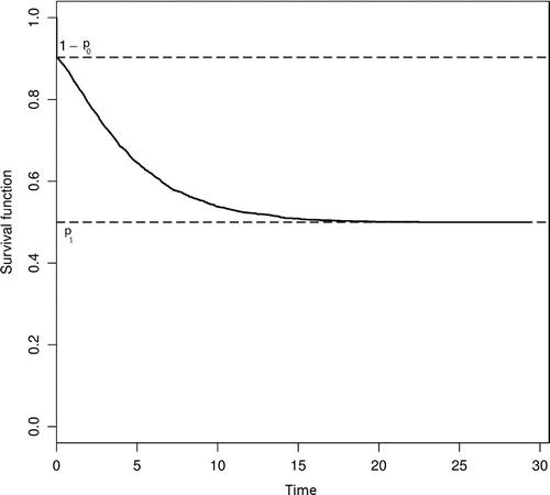
Note that, if $p_0=0$, i.e. without the excess of zeros, we have the cure rate model of Berkson and Gage (1952) (Figure 1).

Figure 1. Survival function of the zero-inflated cure rate model as presented in Louzada, Oliveira, and Moreira (2015).

1.1. Organization

The remainder of this paper is organized as follows. In Section 2, we present a brief review of the literature and preliminary concepts related to the standard promotion time model already used to deal with credit risk modeling. In Section 3, we formulate our proposed model and present the approach for parameter estimation. A study based on Monte Carlo simulations with a variety of parameters is presented in Section 3.2. An application to a real data-set of a Brazilian bank loan portfolio is presented in Section 4. Some general remarks are presented in Section 5.

2. Literature review

In this section, we shall briefly describe the promotion cure rate model studied in Yakovlev and Tsodikov (1996) and Chen, Ibrahim, and Sinha (1999), further extended by Rodrigues, Cancho, de Castro, and Louzada-Neto (2009) among other authors, and thereafter we follow the same notations. This model also incorporates the presence of immune individuals to the event of interest, but still has the disadvantage of not accommodating zero time excess in its framework.

This survival model with a cure fraction, according to Chen et al. (1999), is based on a biological interpretation of the causes that trigger (promote) a cancer disease relapse. As described by the authors, the process that leads to a formation of a detectable cancer mass is triggered by a set of N competitive underlying causes, biologically represented by the number of carcinogenic cells that the individual has left active after the initial treatment. In their paper, it is assumed that N follows a Poisson distribution with mean $\mathit{\theta }$.

Regarding the time until the relapse of the cancer under treatment, Chen et al. (1999) let $Z_i$ be the random time for the ith carcinogenic cells to produce a detectable cancer mass, i.e. the incubation time for the ith (out of N) carcinogenic cell. The random variables $Z_i$, $i=1,2,\dots$, are assumed to be iid, with a common distribution function $F(t)=1-S(t)$, and are independent of N.

In order to include these individuals who are not susceptible to the event of cancer relapse, i.e. the individuals with the initial number of cancer cells, N, equal to 0 and, theoretically, with infinity survival time, it is assumed that $P(Z_0=\infty )=1$.

Finally, the time to the relapse of cancer is defined by the random variable $T=min\{Z_i,0\le i\le N\}$, and therefore, the survival function of T, for the entire population, is given by:(6) $$\begin{array}{cc}\hfill S_p(t)& =P(T>t|N\ge 0)\hfill \\ \hfill & =P(N=0)+P(Z_1>t,\dots ,Z_N>t,N\ge 1)\hfill \\ \hfill & =exp(-\mathit{\theta })+\sum _{k=1}^{\infty }{S(t)}^k\frac{{\mathit{\theta }}^k}{k!}exp(-\mathit{\theta })\hfill \\ \hfill & =exp(-\mathit{\theta }+\mathit{\theta }S(t))=exp(-\mathit{\theta }F(t)).\hfill \end{array}$$(6)

The density function corresponding to (6) is given by $f_p(t)=-\frac{\text{d}}{\text{d}t}{S}_p(t)=\mathit{\theta }f(t)exp(-\mathit{\theta }F(t)).$

We notice that, $S_p$ and $f_p$ are not, properly, survival function and density function, respectively. In fact, note that, $P(Z_0=\infty )=1$, leads to the cure proportion ${lim}_{t\to \infty }{S}_p(t)\equiv S_p(\infty )\equiv P(N=0)=exp(-\mathit{\theta })>0$, which comes from the population of individuals who are not susceptible to the occurrence of cancer relapse (cured). Moreover, the cure fraction is very flexible, i.e. it has the property to accommodate a wide variety of cases, since as $\mathit{\theta }\to \infty$, the proportion of cured tends to 0, as $\mathit{\theta }\to 0$, the proportion of cured tends to 1.

In the situation where we consider the model formulation taking into account only susceptible individuals, that is, when it is present in all individuals a number of initial cancer cells greater than zero, $N\ge 1$, we have a slightly modified expression for the survival function (Chen et al., 1999, p. 910):(7) $$\begin{array}{c}\hfill S_p^{\ast }(t)=P(T>t|N\ge 1)=\frac{exp(-\mathit{\theta }F(t))-exp(-\mathit{\theta })}{1-exp(-\mathit{\theta })}.\end{array}$$(7)

According to this formulation, we figure out now that $S_p^{\ast }(t)$ is a proper survival function, since the following conditions are satisfied: $S_p^{\ast }(0)=1$ and $S_p^{\ast }(\infty )=0$. Still following the model presentation as proposed by Chen et al. (1999), we come to the probability density function of individuals who are susceptible to recurrence of the considered event:(8) $$\begin{array}{cc}\hfill f_p^{\ast }(t)& =-\frac{\text{d}}{\text{d}t}{S}^{\ast }(t)=\left(\frac{exp(-\mathit{\theta }F(t))}{1-exp(-\mathit{\theta })}\right)\mathit{\theta }f(t).\hfill \end{array}$$(8)

Finally, we come to the mathematical relation between the cure rate model, as presented by Berkson and Gage (1952), see expression (1), and the biological based model studied by Chen et al. (1999), among others, in the expression (6):(9) $$\begin{array}{cc}\hfill S_p(t)& =exp(-\mathit{\theta })+(1-exp(-\mathit{\theta }))S_p^{\ast }(t),t\ge 0,\hfill \end{array}$$(9) (10) $$\begin{array}{cc}\hfill f_p(t)& =(1-exp(-\mathit{\theta }))f_p^{\ast }(t),t\ge 0,\hfill \end{array}$$(10)

where $S_p^{\ast }$ and $f_p^{\ast }$ are the proper survival function and the proper density function as given in (7) and (8), respectively. Thus, we see that the Chen et al. (1999) model can be rewritten as a cure rate model, with cure rate equal to $p=exp(-\mathit{\theta })$.

Although the promotion model is formulated within a biological context, it has also been applied in other areas, such as credit risk analysis of bank loan portfolios. In these new developments, the number N is related to the number of risks that compete with the occurrence of a particular financial event of interest, i.e. default or non-performing of loans. Therefore, the formulation admits generalizations in various ways, see for example, Cancho, Suzuki, Barriga, and Louzada (2016). In Barriga, Cancho, and Louzada (2015), the authors studied the time until the event of default on a Brazilian personal loan portfolio, where the authors let N follow a geometric distribution, and F(t) be a cumulative density function of the inverse Weibull distribution.

Furthermore, in the area of credit risk modeling, in Oliveira and Louzada (2014b), the authors applied the model given by (6) to analyze the process underlying the time until full recovery of non-performing loans in a portfolio of personal loans of a Brazilian commercial bank.

In Oliveira and Louzada (2014a), the authors compare the parameters $\mathit{\theta }$ obtained from two follow-up studies of a set of non-performing loans. The first follow-up is related to the time until the default occurrence, while the second one is related to the time until the full recovery of the related loan. The authors found a significant relationship between default and recovery processes. The paper suggests that in times of higher risk of default, it is also likely to have a decrease in the recovery rates of non-performing loans.

3. Model specification

To accommodate zero excess in a survival analysis of loan portfolios, we propose a modification in the survival function of the cure rate model, which has led to the improper survival function given in (3), also labeled as the zero-inflated cure rate model. In this scenario, information from credit risk in loan applications is exploited through the joint modeling of the zero survival times, along with the survival times of the remaining group of borrowers.

The purpose of this paper is to propose a way of incorporating the fraction of zeros into the biological-based promotion cure model. This approach leads the credit risk manager to a complete overview of the risk factors involved in lending, that is, dealing with the likelihood to default on a loan since the loan approval, the non-performing loan control and ensure customer loyalty among long-term survival customers. To exemplify the application of the proposed approach, we analyze a portfolio of loans made available by a large Brazilian commercial bank.

In what follows, we consider the promotion cure rate model as defined in expression (9). Hence, we propose a new (improper) survival function as follows:(11) $$\begin{array}{c}\hfill S_p(t)=p_1+(1-p_0-p_1)S_p^{\ast }(t),t\ge 0,\end{array}$$(11)

where $S_p^{\ast }$ is given by (7), and the parameters $p_0$ and $p_1$ are defined as follows: $p_0=exp(-\mathit{\kappa })$ and $p_1=exp(-\mathit{\theta })$, with $\mathit{\kappa }>0$ and $\mathit{\theta }>0$.

To ensure that $p_0$, $p_1$, and $(1-p_0-p_1)\in (0,1)$, following Pereira, Botter, and Sandoval (2013) and Hosmer and Lemeshow (2000, p. 261), we propose to link two covariate vectors, $x_{1i}$ and $x_{2i}$ into the parameters related to zero inflation and cure rate, respectively, as follows: $p_{0i}=e^{-{\mathit{\kappa }}_i}$, where ${\mathit{\kappa }}_i=-log\left(\frac{e^{x_{1i}^{\top }{\mathit{\beta }}_1}}{1+e^{x_{1i}^{\top }{\mathit{\beta }}_1}+e^{x_{2i}^{\top }{\mathit{\beta }}_2}}\right)$, and $p_{1i}=e^{-{\mathit{\theta }}_i}$, where ${\mathit{\theta }}_i=-log\left(\frac{e^{x_{2i}^{\top }{\mathit{\beta }}_2}}{1+e^{x_{1i}^{\top }{\mathit{\beta }}_1}+e^{x_{2i}^{\top }{\mathit{\beta }}_2}}\right)$, where ${\mathit{\beta }}_1$ is a vector of regression coefficients to be estimated, that relates the influence of the covariates into the excess of zeros, while ${\mathit{\beta }}_2$ is a vector of regression coefficients that relates the influence of the covariates into the cure fraction.

To complete the configuration of the model, i.e. to determine the parametric form of $S_p^{\ast }$, we let f(t) and F(t) be, respectively, the density probability function and the cumulative probability function of the Weibull distribution. This could be done in a more general way, but for didactic reasons we prefer to choose a particular distribution to present our methodology. The Weibull distribution is a continuous probability distribution, commonly applied in survival analysis and reliability. It has two parameters, ${\mathit{\alpha }}_1>0$ and ${\mathit{\alpha }}_2>0$, respectively, the shape and scale parameters. Therefore, we link the Weibull parameters as follows: ${\mathit{\alpha }}_{1i}=e^{x_{3i}^{\top }{\mathit{\beta }}_3}$ and ${\mathit{\alpha }}_{2i}=e^{x_{4i}^{\top }{\mathit{\beta }}_4}$. These are the most convenient links because $g_1(·)$ and $g_2(·)$ are link functions strictly monotonic and twice differentiable that map ${\mathbb{R}}^{+}$ into $\mathbb{R}$. Finally, we present the following framework for the zero-inflated promotion cure rate model:(12) $$\begin{array}{cc}\hfill S_p(t)& =exp(-\mathit{\theta })+(1-exp(-\mathit{\kappa })-exp(-\mathit{\theta }))S_p^{\ast }(t),\hfill \\ \hfill S_p^{\ast }(t)& =\frac{exp(-\mathit{\theta }F(t))-exp(-\mathit{\theta })}{1-exp(-\mathit{\theta })},\hfill \\ \hfill f_p^{\ast }(t)& =\left(\frac{exp(-\mathit{\theta }F(t))}{1-exp(-\mathit{\theta })}\right)\mathit{\theta }f(t),\hfill \\ \hfill F(t)& =1-e^{-{\left(\frac{t}{\mathit{\theta }}\right)}^{\mathit{\alpha }}}\text{and}\hfill \\ \hfill f(t)& =\frac{\mathit{\alpha }}{\mathit{\theta }}{\left(\frac{t}{\mathit{\theta }}\right)}^{\mathit{\alpha }-1}{e}^{{\left(-\frac{t}{\mathit{\theta }}\right)}^{\mathit{\alpha }}}.\hfill \end{array}$$(12)

3.1. Likelihood function

Regarding the contribution of each customer for the likelihood function, we must note that there are different sub-groups of customers: (i) individual with event at the starting time (zero time), (ii) non-susceptible for the event, or (iii) susceptible for the event. The expression (13) presents the likelihood contribution of each time to default $t_i$:(13) $$\begin{array}{c}\hfill \left\{\begin{array}{cc}{p}_{0i},\hfill & \text{if}{t}_i=0,\hfill \\ (1-p_{0i}-p_{1i})f_p^{\ast }(t_i),\hfill & \text{if}{t}_i\text{is fully observed}\hfill \\ p_{1i}+(1-p_{0i}-p_{1i})S_p^{\ast }(t_i),\hfill & \text{if}{t}_i\text{is right censored}.\hfill \end{array}\right.\end{array}$$(13)

Let the data take the form $\mathcal{D}=\left\{t_i,{\mathit{\delta }}_i,x_i=\{x_{1i},x_{2i},x_{3i},x_{4i}\}\right\}$, where ${\mathit{\delta }}_i=1$ if $t_i$ is an observable time to default, ${\mathit{\delta }}_i=0$ if it is right censored, for $i=1,2,\dots ,n,$ and $x_i$ is vector of covariates associated with a customer i. As we shall see in the application section, the covariate vectors can be the same, i.e. $x_1=x_3=x_2=x_4$. Let $({\mathit{\alpha }}_1,{\mathit{\alpha }}_2)$ denote the parameter vector of the Weibull distribution and, finally, let $({\mathit{\beta }}_{\mathit{\kappa }},{\mathit{\beta }}_{\mathit{\theta }})$ be the regression parameters associated, respectively, with the proportion of inflation of zeros and the proportion of long-term survivors (cure rate).

The likelihood function of the proposed new zero-adjusted cure rate survival model, with a parameter vector, $\mathit{\vartheta }=({\mathit{\alpha }}_1,{\mathit{\alpha }}_2,{\mathit{\beta }}_{\mathit{\kappa }},{\mathit{\beta }}_{\mathit{\theta }})$, to be estimated via the MLE approach is based on a sample of n observations, $\mathcal{D}=\left\{t_i,{\mathit{\delta }}_i,x\right\}$. Finally, we write the likelihood function, under non-informative censoring, as:(14) $$\begin{array}{c}\hfill L(\mathit{\vartheta };\mathcal{D})\propto \prod _{t_i=0}\left\{p_{0i}\right\}\prod _{t_i>0}\left\{{\left[(1-p_{0i}-p_{1i})f_p^{\ast }(t_i)\right]}^{{\mathit{\delta }}_i}{\left[p_{1i}+(1-p_{0i}-p_{1i})S_p^{\ast }(t_i)\right]}^{1-{\mathit{\delta }}_i}\right\}\end{array}$$(14)

The maximum likelihood estimates $\widehat{\mathit{\vartheta }}=(\widehat{{\mathit{\alpha }}_1},\widehat{{\mathit{\alpha }}_2},\widehat{{\mathit{\beta }}_{\mathit{\kappa }}},\widehat{{\mathit{\beta }}_{\mathit{\theta }}})$ can be obtained by solving the non-linear system of equations $U(\mathit{\vartheta })=\frac{\mathit{\partial }l(\mathit{\vartheta })}{\mathit{\partial }\mathit{\vartheta }}=0$. We use the free statistical software R to solve them numerically using iterative techniques, such as the Newton–Raphson algorithm. The computational code is available from the authors upon request.

Following Migon, Gamerman, and Louzada (2014) and Ospina and Ferrari (2012), a large sample inference for the parameters is based on the matrix of second derivatives of the log likelihood using the observed information matrix, $\mathbf{I}(\mathit{\vartheta })={\{-{\mathit{\partial }}^2\ell (\mathit{\vartheta })/\mathit{\partial }\mathit{\vartheta }\mathit{\partial }{\mathit{\vartheta }}^T\}}^{-1}$, evaluated at $\mathit{\vartheta }=\widehat{\mathit{\vartheta }}$. The approximate $(1-\mathit{\alpha })$ 100% confidence intervals for the parameters ${\mathit{\alpha }}_1,{\mathit{\alpha }}_2,{\mathit{\beta }}_{\mathit{\kappa }}$ and ${\mathit{\beta }}_{\mathit{\theta }}$ are given by ${\widehat{\mathit{\alpha }}}_1\pm {\mathit{\xi }}_{\mathit{\alpha }/2}\sqrt{\text{Var}({\widehat{\mathit{\alpha }}}_1)}$, ${\widehat{\mathit{\alpha }}}_2\pm {\mathit{\xi }}_{\mathit{\alpha }/2}\sqrt{\text{Var}({\widehat{\mathit{\alpha }}}_2)}$, $\widehat{{\mathit{\beta }}_{\mathit{\kappa }}}\pm {\mathit{\xi }}_{\mathit{\alpha }/2}\sqrt{\text{Var}(\widehat{{\mathit{\beta }}_{\mathit{\kappa }}})}$ and $\widehat{{\mathit{\beta }}_{\mathit{\theta }}}\pm {\mathit{\xi }}_{\mathit{\alpha }/2}\sqrt{\text{Var}(\widehat{{\mathit{\beta }}_{\mathit{\theta }}})}$, where ${\mathit{\xi }}_{\mathit{\alpha }/2}$ is the upper $\mathit{\alpha }/2$ percentile of the standard normal distribution.

In the application section, we compare the proposed model configured with different covariates. A comparison of the models was made using the selection criterion known as the Akaike information criterion (AIC), proposed by Akaike (1974). The criterion is defined by $\text{AIC}=-2\text{log}(L)+2k$, where k is the number of estimated parameters, n the sample size and L is the maximised value of the likelihood function. The model with the smallest value is chosen as the preferred for describing a given data-set among all models considered.

3.2. Simulation algorithm

Suppose that the time of occurrence of an event of interest has the improper cumulative distribution function F(t) given by $F(t)=p_0+(1-p_0-p_1)F_0(t),t\ge 0.$ We aim to simulate random samples of size n posing as loan survival times, where each sample comprises a proportion $p_0$ of zero-inflated times, a non-default fraction of $p_1$ and with a proportion $(1-p_0-p_1)$, of failure times drawn from a Weibull distribution with ${\mathit{\alpha }}_1$ and ${\mathit{\alpha }}_1$ parameters.

For the purpose of simulation, we let x be a random variable that represents a customer characteristic. Hence, the link configuration of the eight parameters $({\mathit{\beta }}_{10}$, ${\mathit{\beta }}_{11}$, ${\mathit{\beta }}_{20}$, ${\mathit{\beta }}_{21}$, ${\mathit{\beta }}_{30}$, ${\mathit{\beta }}_{31}$, ${\mathit{\beta }}_{40}$, ${\mathit{\beta }}_{41})$ to be estimated is given by the following expressions:(15) $$\begin{array}{cc}\hfill {\mathit{\kappa }}_i& =-log\left(\frac{e^{{\mathit{\beta }}_{10}+x_i{\mathit{\beta }}_{11}}}{1+e^{{\mathit{\beta }}_{10}+x_i{\mathit{\beta }}_{11}}+e^{{\mathit{\beta }}_{20}+x_i{\mathit{\beta }}_{21}}}\right),\hfill \\ \hfill {\mathit{\theta }}_{1i}& =-log\left(\frac{e^{{\mathit{\beta }}_{20}+x_i{\mathit{\beta }}_{21}}}{1+e^{{\mathit{\beta }}_{10}+x_i{\mathit{\beta }}_{11}}+e^{{\mathit{\beta }}_{20}+x_i{\mathit{\beta }}_{21}}}\right),\hfill \\ \hfill {\mathit{\alpha }}_{1i}& =e^{{\mathit{\beta }}_{30}+x_i{\mathit{\beta }}_{31}},\hfill \\ \hfill {\mathit{\alpha }}_{2i}& =e^{{\mathit{\beta }}_{40}+x_i{\mathit{\beta }}_{41}}.\hfill \end{array}$$(15)

Considering the parameters established in the regression model defined above, we set three different scenarios of parameters for the simulation studies performed here. Playing the role of covariate, we assume x as a binary covariate with values drawn from a Bernoulli distribution with parameter 0.5.

For scenario 1, ${\mathit{\beta }}_{10}$ assumes $-3$ and ${\mathit{\beta }}_{11}$ assumes 1. ${\mathit{\beta }}_{20}$ assumes $-2$ and ${\mathit{\beta }}_{21}$ assumes 0.75. Given that the assumed values of x are 0 and 1, we have that $p_0$ assumes, respectively, 4.20 and 9.51%, while $p_1$ assumes 11.41 and 20.15%. Compared to the other scenarios 2 and 3, scenario 1 has the characteristic of having a low rate of STD and non-default. Regarding the Weibull parameters, ${\mathit{\beta }}_{30}$ assumes 0.5, ${\mathit{\beta }}_{31}$ assumes 0.5, ${\mathit{\beta }}_{40}$ assumes 1.5 and ${\mathit{\beta }}_{41}$ assumes 2. This implies that the Weibull parameter ${\mathit{\alpha }}_1$ can assume 1.64 or 2.71 values, while ${\mathit{\alpha }}_2$ assumes 4.48 or 33.11.

For scenario 2, ${\mathit{\beta }}_{10}$ assumes $-2$ and ${\mathit{\beta }}_{11}$ assumes 1.5. ${\mathit{\beta }}_{20}$ assumes $-1.25$ and ${\mathit{\beta }}_{21}$ assumes 1. Given that the assumed values of x are 0 and 1, we have that $p_0$ assumes, respectively, 9.51 and 25.42%, while $p_1$ assumes 20.15 and 32.64%. Compared to the other scenarios 1 and 3, scenario 2 has the characteristic of having a moderate rate of STD and non-default. Regarding the Weibull parameters, ${\mathit{\beta }}_{30}$ assumes $-0.5$, ${\mathit{\beta }}_{31}$ assumes 1.5, ${\mathit{\beta }}_{40}$ assumes $-0.75$ and ${\mathit{\beta }}_{41}$ assumes 3. This implies that the Weibull parameter ${\mathit{\alpha }}_1$ can assume 0.60 or 2.71 values, while ${\mathit{\alpha }}_2$ assumes 0.47 or 9.48.

For scenario 3, ${\mathit{\beta }}_{10}$ assumes $-1$ and ${\mathit{\beta }}_{11}$ assumes 1. ${\mathit{\beta }}_{20}$ assumes -1 and ${\mathit{\beta }}_{21}$ assumes 1. Given that the assumed values of x are 0 and 1, we have that $p_0$ assumes, respectively, 21.20 and 33.33%, while $p_1$ assumes 20.20 and 33.33%. Compared to the other scenarios 1 and 2, scenario 3 has the characteristic of having a high rate of STD and non-default. Regarding the Weibull parameters, ${\mathit{\beta }}_{30}$ assumes $-0.75$, ${\mathit{\beta }}_{31}$ assumes 1, ${\mathit{\beta }}_{40}$ assumes 1.25 and ${\mathit{\beta }}_{41}$ assumes 1. This implies that the Weibull parameter ${\mathit{\alpha }}_1$ can assume 0.42 or 1.28 values, while ${\mathit{\alpha }}_2$ assumes 3.49 or 9.48.

The following step-by-step algorithm is based on the afore-mentioned link functions associated with an x covariate drawn from a Bernoulli distribution with parameter 0.5, representing a customer feature.

(1)	Set ${\mathit{\beta }}_{10}$ and ${\mathit{\beta }}_{11}$ related to the value of the desired proportion of zero-inflated times, $p_0$, along with ${\mathit{\beta }}_{20}$ and ${\mathit{\beta }}_{21}$ related to the value of the desired non-default fraction, $p_1$; finally, set the Weibull parameters ${\mathit{\beta }}_{30}$ and ${\mathit{\beta }}_{31}$ related to ${\mathit{\alpha }}_1$, ${\mathit{\beta }}_{40}$ and ${\mathit{\beta }}_{41}$ related to ${\mathit{\alpha }}_2$;
(2)	Draw $x_i$ from $x\sim$ Bernoulli (0.5) and calculate $p_{0i}$, $p_{1i}$, ${\mathit{\alpha }}_{1i}$ and ${\mathit{\alpha }}_{2i}$;
(3)	Generate $u_i$ from a uniform distribution $U(0,1)$;
(4)	If $u_i\le p_{0i}$, set $s_i=0$;
(5)	If $u_i>1-p_{1i}$, set $s_i=\infty$;
(6)	If $p_{0i}<u_i\le 1-p_{1i}$, generate $v_i$ from a uniform distribution U$(p_{0i},1-p_{1i})$ and take $s_i$ as the root of $F(s_i)-v_i=0$;
(7)	Generate $w_i$ from a uniform $U(0,max(s_i))$, considering only finites $s_i$;
(8)	Calculate $t_i=min(s_i,w_i)$, if $t_i<w_i$, set ${\mathit{\delta }}_i=1$, otherwise, set ${\mathit{\delta }}_i=0$.
(9)	Repeat as necessary from step 2 until you get the desired amount of sample $(t_i,{\mathit{\delta }}_i)$.

Note that the censoring distribution chosen is a uniform distribution with limited range in order to keep the censoring rates reasonable (see Rocha, Nadarajah, Tomazella, Louzada, & Eudes, 2015, p. 12).

Figure 2. Bias, square root of mean squared error and coverage probability (CP) of the maximum likelihood estimation $({\widehat{\mathit{\beta }}}_{10}$, ${\widehat{\mathit{\beta }}}_{11}$, ${\widehat{\mathit{\beta }}}_{20}$, ${\widehat{\mathit{\beta }}}_{21})$ of zero-inflated promotion cure rate regression model for simulated data under the three scenarios of parameters, obtained from Monte Carlo simulations with 1,000 replications and increasing sample size (n). 1 indicates scenario 1 with characteristic of having a low rate of STD and non-default. 2 indicates the scenario 2 with characteristic of having a moderate rate of STD and non-default. 3 indicates scenario 3 with a characteristic of having a high rate of STD and non-default.

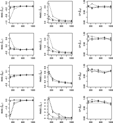
Figure 3. Bias, square root of mean squared error and coverage probability (CP) of the maximum likelihood estimation $({\widehat{\mathit{\beta }}}_{30}$, ${\widehat{\mathit{\beta }}}_{31}$, ${\widehat{\mathit{\beta }}}_{40}$, ${\widehat{\mathit{\beta }}}_{41})$ of zero-inflated promotion cure rate regression model for simulated data under the three scenarios of parameters, obtained from Monte Carlo simulations with 1,000 replications and increasing sample size (n). 1 indicates the scenario 1 with characteristic of having a low rate of STD and non-default. 2 indicates the scenario 2 with characteristic of having a moderate rate of STD and non-default. 3 indicates scenario 3 with characteristic of having a high rate of STD and non-default.

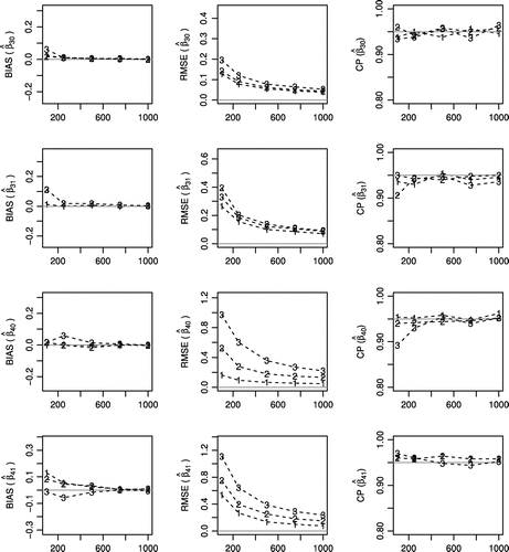
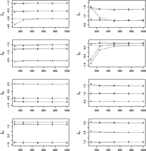
Figure 4. MLEA, maximum likelihood estimation on average of the parameters $({\widehat{\mathit{\beta }}}_{10}$, ${\widehat{\mathit{\beta }}}_{11}$, ${\widehat{\mathit{\beta }}}_{20}$, ${\widehat{\mathit{\beta }}}_{21}$, ${\widehat{\mathit{\beta }}}_{30}$, ${\widehat{\mathit{\beta }}}_{31}$, ${\widehat{\mathit{\beta }}}_{40})$, ${\widehat{\mathit{\beta }}}_{41}$ of zero-inflated Promotion Cure rate regression model for simulated data under the three scenarios of parameters, obtained from Monte Carlo simulations with 1,000 replications and increasing sample size (n). 1 indicates the scenario 1 with characteristic of having a low rate of STD and non-default. 2 indicates scenario 2 with characteristic of having a moderate rate of STD and non-default. 3 indicates the scenario 3 with characteristic of having a high rate of STD and non-default.

3.3. Results of Monte Carlo simulations

The followings Figures 2–4, describe the simulation results for the three simulated scenarios of parameters, where the sample size varies as $n=100$, 250, 500, 750, and 1,000.

The parameter values are selected in order to assess the ML estimation performance under different shape and scale parameters (${\mathit{\beta }}_{30}$, ${\mathit{\beta }}_{31}$, ${\mathit{\beta }}_{40}$ and ${\mathit{\beta }}_{41}$, related to the Weibull time-to-default distribution), and also under a composition of different proportions of zero-inflated data (${\mathit{\beta }}_{10}$ and ${\mathit{\beta }}_{11}$) and non-defaulters rates (${\mathit{\beta }}_{20}$ and ${\mathit{\beta }}_{21}$ related to censored data). It can be seen from the figures that:

(1)	in general, the maximum likelihood estimation on average, MLEA, is close to the parameters set in the simulated parameter scenarios, see Figure 4. However, in scenarios 1 and 2, the parameters ${\widehat{\mathit{\beta }}}_{11}$ and ${\widehat{\mathit{\beta }}}_{21}$ need a larger sample size (from at least n = 500 for ${\mathit{\beta }}_{21}$) to achieve convergence.
(2)	in general, according to Figures 2 and 3, biases and root-mean-square errors decrease as the sample size increases; we also observe that, in general, the coverage probability, i.e. the proportion of the time that the interval contains the true value of interest, is close to 95%, as expected;
(3)	in the scenarios with the greatest presence of non-default and zeros, i.e. scenario 2 (Moderate) and 3 (High), the MLEA, and the measures of RMSE, Bias and CP of the estimated regression parameters related to $p_0=exp(-\mathit{\kappa })$ and $p_1=exp(-\mathit{\theta })$, performs better compared to scenario 1 (Low), due, of course, to greater presence of zeros and censored data;
(4)	on the other hand, in the scenario with the fewer presence of zeros and non-default and, i.e. scenario 1 (Low), the MLEA, and the measures of RMSE, Bias and CP of the estimated regression parameters related to ${\mathit{\alpha }}_1$ and ${\mathit{\alpha }}_2$, performs better compared to other scenarios, due to the greater presence of observed time-to-default data;

4. Application: Brazilian bank loan portfolio

4.1. Real data-set

This section presents a data-set made available by a major Brazilian bank. It is important to note that the presented data-sets, amounts, rates and levels of the available covariates do not necessarily represent the actual condition of the financial institution’s portfolio. That is, despite being a real database, the bank may have sampled the data in order to change the current status of its loan portfolio.

The analyzed portfolio was collected from customers who have taken out a personal loan over a 60-month period, between 2010 and 2015. Table 1 shows the customer’s quantitative frequencies of the loan portfolio provided by the bank. comprises 5,733 time to default (in months), with an approximate 80% rate of censored data, that is, a high rate of non-default loans. Our objective is to assess if customer characteristics are associated with time-to-default (credit risk) patterns of each of the three types of clients: the group with time to default equal to zero, i.e. the zero-inflated ones who we called straight-to-default clients (STD) loans; the positive time to default due to defaulted loans; and finally, the class of censored observations due to the high non-default rate shown in the data.

Table 1. Frequency and percentage of the bank loan lifetime data

Number of customers	Number of STD ($T=0)$	Number of defaulters $(T>0)$	Number of censored $(T=\infty )$
5,733	321 (5.60%)	810 (14.13%)	4,602 (80.27%)

The segmentation of customers of the bank was made a priori by the bank. For example, age group 1 means that customers have been grouped by age from a specified range (determined by the bank). The classification of the type of residence, type of employment and age group has not been fully supplied to our study due to confidentiality issues. For instance, we do not even know if age group 1 comprises a class of clients younger than ones from age group 4. Table 2 shows the quantitative frequency according to the available covariates.

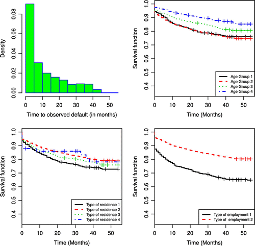
Figure 5 presents a graphical summary of the survival behavior present in the available covariates: age group, type of residence, and type of employment. The histogram shows only the distribution of the observed data, while the censored data are better observed through the KM curves. Notwithstanding, we can see the presence of zero-inflated data in both. We can see from the stratified Kaplan–Meier survival curves that the age group identified as 4 has a lower presence of zero-inflated time (STD borrowers) compared to the others. The group with type of residence 4 shows a higher presence of zero-inflated time (STD borrowers) compared to the borrowers with other types of residences. The type of employment 2 shows clearly a high non-default rate and it also presents a lower rate of zero-inflated times.

Table 2. Quantity of the available covariates

Covariate	Quantity of customers
Age group 1	503
Age group 2	3,088
Age group 3	1,220
Age group 4	922
Type of residence 1	629
Type of residence 2	4,056
Type of residence 3	998
Type of residence 4	50
Type of employment 1	956
Type of employment 2	4,777

Figure 5. Brazilian bank loan portfolio data.

Notes: Top panel, shows a histogram for the observed time-to-default variable of interest (left) and Kaplan–Meier survival curves stratified by age group (right). Bottom panel, Kaplan–Meier survival curves stratified by type of residence (left) and Kaplan–Meier survival curves stratified by type of employment (right).

4.2. Modeling results

In this section, we present the application of the zero-inflated promotion cure rate regression model introduced in Section 3. In order to proceed the model fit, we considered dummy covariates for all levels of the available covariates. Therefore, including all the intercepts, we might have up to thirty two ($32=4\times 4\times 2$) regression parameters to be estimated. To reach the final model, variables were selected in a backward elimination way using the p-values of the Wald test and AIC.

Table 3 summarizes the estimated parameters via MLE approach for the regression parameters. The final model has AIC of 12,596.26 ($l\{{\widehat{\mathit{\beta }}}_{10},{\widehat{\mathit{\beta }}}_{11},{\widehat{\mathit{\beta }}}_{12},{\widehat{\mathit{\beta }}}_{13},{\widehat{\mathit{\beta }}}_{20},{\widehat{\mathit{\beta }}}_{21},{\widehat{\mathit{\beta }}}_{22},{\widehat{\mathit{\beta }}}_{30},{\widehat{\mathit{\beta }}}_{40},{\widehat{\mathit{\beta }}}_{41}\}=-6288.128,p=10)$.

Table 3. The zero-inflated promotion cure regression model for time to default on a Brazilian bank loan portfolio

Parameter	Dummy covariate (param${}^{(1)}$)	Estimate	S.E.${}^{(2)}$	p-value	Exp.${}^{(3)}$
$p_0$	Intercept $({\mathit{\beta }}_{10})$	$-0.6690$	0.1213	0.0000	0.5122
	Age group =4 $({\mathit{\beta }}_{11})$	$-0.8187$	0.2231	0.0002	0.4409
	Type of residence = 4 $({\mathit{\beta }}_{12})$	0.8653	0.4736	0.0677	2.3757
	Type of employment = 2 $({\mathit{\beta }}_{13})$	$-0.6473$	0.1434	0.0000	0.5234
$p_1$	Intercept $({\mathit{\beta }}_{20})$	0.9123	0.0957	0.0000	2.4901
	Type of residence = 1 $({\mathit{\beta }}_{21})$	$-0.2905$	0.1028	0.0047	0.7478
	Type of employment = 2 $({\mathit{\beta }}_{22})$	0.6331	0.0970	0.0000	1.8834
${\mathit{\alpha }}_1$	Intercept $({\mathit{\beta }}_{30})$	0.1730	0.0376	0.0000	1.1889
${\mathit{\alpha }}_2$	Intercept $({\mathit{\beta }}_{40})$	3.1855	0.0697	0.0000	24.1817
	Age group = 4 $({\mathit{\beta }}_{41})$	0.6895	0.1435	0.0000	1.9927

${}^1$ Related regression parameter to be estimated; ${}^2$ Standard error; ${}^3$ Exponentiation of the estimated parameter.

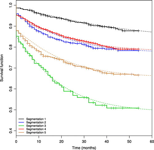
The selected dummy covariates given in the final model enabled us to split the portfolio between 12 five different groups of borrowers (segmentations). In Figure 6, we present the estimated survival curves (the dotted lines), among with the Kaplan–Meier survival curves considering the reached segmentation: segmentation 1 comprises borrowers with the following set of attributes: age group equal to 4, type of residence equal to 2 or 3 and type of employment equal to 2; segmentation 2 comprises borrowers with the following set of attributes: age group not equal to 4, type of residence equal to 1 and type of employment equal to 2; segmentation 3 comprises borrowers with the following set of attributes: age group not equal to 4, type of residence equal to 1 and type of employment equal to 1; segmentation 4 comprises borrowers with the following set of attributes: age group not equal to 4, type of residence equal to 2 or 3 and type of employment equal to 2; and, finally, segmentation 5 comprises borrowers with the following set of attributes: age group not equal to 4, type of residence equal to 2 or 3 and type of employment equal to 1.

Figure 6 shows the adjusted survival curves according to the parameters obtained MLE approach.

Figure 6. Brazilian bank loan portfolio. Kaplan–Meier survival curves stratified through the covariate selection given by the final promotion cure rate regression model presented in the Table 3.

5. Concluding remarks

We introduced a methodology based on zero-inflated survival data that extends the model studied in Yakovlev and Tsodikov (1996) and Chen et al. (1999). Considering this, an advantage of our approach is to accommodate zero-inflated times, which is not possible in the standard cure rate model. To illustrate the methodology presented here, we analyzed a bank loan survival data, in order to assess the propensity to default in loan applications. In this scenario, information from borrowers is exploited through the joint modeling of the zero survival time, along with the survival times of the remaining portfolio. The results showed the new model performed very well, nonetheless, it is important to note that the actual performance of novel models will be measured considering its daily use by the bank and using a wider variety of available covariates, since the model allows the use of as many covariates as needed, whether continuous or categorical.

Identifiability issues of the cure rate model in (1) and the promotion cure model (6) are discussed in Li, Taylor, and Sy (2001). According to Mateluna (2014), the authors concluded that in both cases, it is necessary to include covariates in the cure fractions to make them identifiable. From Peng and Zhang (2008), identifiability for the promotion cure model can be ensured when covariates are included in both parameters related to the susceptible fraction and the cure fraction of individuals (see Mateluna, 2014, p. 28).

Although we have included one more parameter in both models mentioned above, identifiability issues will not be discussed in this paper. This important subject is intended to be addressed in future research.

Acknowledgements

We are grateful to the Editorial Board and the reviewers for their valuable comments and suggestions which has improved the manuscript.

Additional information

Funding

This research was sponsored by CAPES Process number: BEX 10583/14-9, Brazil.

Notes on contributors

Mauro Ribeiro de Oliveira

Mauro Ribeiro de Oliveira Jr holds a PhD in Statistics from the Federal University of São Carlos and has experience in the area of Probability and Statistics, with emphasis on Credit Risk Modeling. He is currently an employee of Caixa EconÔmica Federal.

Fernando Moreira

Fernando Moreira holds a PhD in Management Science and Business Economics from the University of Edinburgh, and has previously worked for the Central Bank of Brazil (Supervision Department). After graduating, he worked at Keele University as a lecturer in Finance before returning to the University of Edinburgh as a lecturer in Business Economics.

Francisco Louzada

Francisco Louzada is a professor of Statistics at the Institute for Mathematical Science and Computing, University of São Paulo (USP), Brazil. He received his PhD degree in Statistics from the University of Oxford, UK, his MSc degree in Computational Mathematics from USP, Brazil, and his BSc degree in Statistics from UFSCar, Brazil. His main research interests are in survival analysis, data mining, Bayesian inference, classical inference, and probability distribution theory.

References

- Akaike, H. (1974). A new look at the statistical model identification. IEEE Transactions on Automatic Control, 19(6), 716–723.
- Barriga, G. D., Cancho, V. G., & Louzada, F. (2015). A non-default rate regression model for credit scoring. Applied Stochastic Models in Business and Industry, 31(6), 846–861.
- Berkson, J., & Gage, R. P. (1952). Survival curve for cancer patients following treatment. Journal of the American Statistical Association, 47(259), 501–515.
- Cancho, V. G., Suzuki, A. K., Barriga, G. D., & Louzada, F. (2016). A non-default fraction bivariate regression model for credit scoring: An application to brazilian customer data. Communications in Statistics: Case Studies, Data Analysis and Applications, 2(1), 1–12.
- Chen, M.-H., Ibrahim, J. G., & Sinha, D. (1999). A new Bayesian model for survival data with a surviving fraction. Journal of the American Statistical Association, 94, 909–919.
- Hosmer, D. W., & Lemeshow, S. (2000). Applied Logistic Regression (2nd ed.). New York, NY: John Wiley and Sons.
- Li, C.-S., Taylor, J. M., & Sy, J. P. (2001). Identifiability of cure models. Statistics & Probability Letters, 54(4), 389–395.
- Louzada, F., Oliveira, M. R., & Moreira, F. F. (2015). The zero-inflated cure rate regression model: Applications to fraud detection in bank loan portfolios. arXiv preprint arXiv:1509.05244.
- Mateluna, D. I. G. (2014). Extensões em modelos de sobrevivência com fração de cura e efeitos aleatórios (Ph.D. thesis). Universidade de São Paulo, S{\~a}o Paulo.
- Migon, H. S., Gamerman, D., & Louzada, F. (2014). Statistical inference: An integrated approach. CRC Press.
- Oliveira, M. R., & Louzada, F. (2014a). An evidence of link between default and loss of bank loans from the modeling of competing risks. Singaporean Journal of Business Economics and Management Studies, 3(1), 30–37.
- Oliveira, M. R., & Louzada, F. (2014b). Recovery risk: Application of the latent competing risks model to non performing loans. Tecnologia de Crédito, 88, 43–53.
- Ospina, R., & Ferrari, S. L. (2012). A general class of zero-or-one inflated beta regression models. Computational Statistics & Data Analysis, 56(6), 1609–1623.
- Othus, M., Barlogie, B., LeBlanc, M. L., & Crowley, J. J. (2012). Cure models as a useful statistical tool for analyzing survival. Clinical Cancer Research, 18(14), 3731–3736.
- Peng, Y., & Zhang, J. (2008). Identifiability of a mixture cure fraitly model. Statistics & Probability Letters, 78, 2604–2608.
- Pereira, G. H., Botter, D. A., & Sandoval, M. C. (2013). A regression model for special proportions. Statistical Modelling, 13(2), 125–151.
- Rocha, R., Nadarajah, S., Tomazella, V., Louzada, F., & Eudes, A. (2015). New defective models based on the kumaraswamy family of distributions with application to cancer data sets. Statistical Methods in Medical Research, 1–23.
- Rodrigues, J., Cancho, V. G., de Castro, M., & Louzada-Neto, F. (2009). On the unification of long-term survival models. Statistics & Probability Letters, 79(6), 753–759.
- Tong, E. N., Mues, C., & Thomas, L. C. (2012). Mixture cure models in credit scoring: If and when borrowers default. European Journal of Operational Research, 218(1), 132–139.
- Yakovlev, A. Y., & Tsodikov, A. D. (1996). Stochastic models of tumor latency and their biostatistical applications. Singapore: World Scientific.