A multi-factor model of heterogeneous traders in a dynamic stock market

Abstract

This study develops an agent-based computational stock market model in which each trader’s buying and selling decisions are endogenously determined by multiple factors: namely, firm profitability, past stock price movement, and imitation of other traders. Each trader can switch from being a buyer to a seller, and vice versa, depending on market conditions. Simulation findings imply liquidity in the stock market decreases as more traders try to behave in a similar way to other traders. Stock return volatility is increasing in memory length when the information set of a trader includes only the fundamental of stock. On the other hand, when all traders consider only the past stock price movement, stock prices undergo boom and bust cycles with the occasional no-trade states. Furthermore, when traders consider three factors equally, the stock return is characterized by more pronounced fat-tail property and lower volatility.

Keywords:

• heterogeneous trader
• memory length
• asset pricing
• agent-based stock market

AMS Subject Classifications:

• G11
• G12
• G17

Public Interest Statement

This paper builds an agent-based computational stock market model to examine how simple behavioral trading rules by agents affect the asset price dynamics. In the model, the information set of a trader includes firm profitability, past stock price movement, and investment decisions by neighboring traders. Stock market dynamics are quite different depending on what factors are employed. When all traders attempt to mimic each other, the no-trade state quickly emerges. We also find the stock return volatility varies by the memory length of a trader, the extent of use of historical stock market data. It is also shown the fat-tail property in the stock return distribution is more pronounced when traders consider three factors equally. Interestingly, when all traders only respond the past stock return, stock prices are characterized by the boom and bust cycle.

1. Introduction

This study builds an agent-based computational stock market¹ that allows us to investigate various aspects of the stock market when traders use simple behavioral trading rules, which are based on empirical observations on how people make financial investments.

In the model, traders allocate their wealth between a risky stock and a risk-free asset based on heterogeneous information sets. The information set of each trader can include data on three factors: firm profitability, the past stock return movement, and the investment behavior of other traders with whom a trader interacts. The behavioral assumption on portfolio rebalancing used in this study is based on a mixture of network effect² and momentum strategies.

While the current literature focuses on endogenous switching between a few trading types (i.e. chartists and fundamentalists), we rather view agents as standing somewhere between extreme types. Rather than imposing endogenous selection among different forecasting rules, we take a shortcut: demand or supply is a direct function of the factors described. This could be understood as there exists a sort of internal forecasting mechanism that converts the information set to a specific investment rule.³

take a similar approach in their study of a double auction stock market. The distinctive feature of their model is that a trader forms an expectation about future stock returns based on multiple components, i.e. fundamentalist component, chartist component, and the noise component. What differentiates our model from Chiarella et al. (2009) is that we replace the fundamental price by the subjective perception of a trader on current firm profitability relative to the history of it.⁴ Also, subjective evaluation of each component does not go through expectation formation process. Rather, they are directly blended into portfolio choice.

One of the key advantages of exploiting multiple factors in forming portfolio decision is that we have a flexible platform which allows us to explore how heterogeneous responses to each of factors affect stock market dynamics. For example, it would be worthwhile to see how the system reacts to conflicting signals about asset valuation, i.e. low profitability coupled with past high stock return.

It should be noted that subjective comparison of current firm profitability relative to past profitability inherently involves selection of extent of past data usage (i.e. memory length). In this study, the relative profitability of the firm is represented as the normalized deviation of current dividend to moving average of the dividend. Memory length in using past information and heterogeneous learning gain is shown to be crucial aspects of market dynamics in LeBaron (2001a, b, 2012). As we will see in the following sections, our model also generates quite different market dynamics under different schemes of memory length.

Another distinction between this study and previous computational stock market studies is that our model permits the endogenous determination of trading positions and no-trade states. A no-trade state is a situation where all traders are on the same side of trading direction for any values in the space of stock price. This feature has rarely been examined in a majority of computational stock market models since it is conventional to assume that there always is a fixed amount of stock shares that are ready to be supplied. This assumption is analogous to saying there is a continuous IPO market in each trading period. We circumvent this unrealistic convention by postulating that a trader’s demand or supply for stocks is dependent on his current state.

This study critically departs from the earlier literature in an additional way; the portfolio choice of a trader is directly influenced by the portfolio profile of linked traders. The mimetic behavior could be expressed as the following: if my friends buy more stock, I would also buy more.⁵ We model stock holdings of a trader as a function of stock holdings of agents within his interacting boundaries. The rationale for this type of assumption can be found in numerous works in the empirical finance literature that show the significance of social influence on financial investment behavior (e.g. Brown, Ivković, Smith, & Weisbenner, 2008; Hong, Kubik, & Stein, 2004; Hong, Kubik, & Stein, 2005; Malloy, Frazzini, & Cohen, 2008; Shiller & Pound, 1989).

Key simulation findings are as follows. If all traders only take into account firm dividend as a key informational factor, and the dividend process is non-stationary, then long-memory dividend traders create a more volatile stock return process than short-memory dividend traders. For the stock market with traders who care about only a prior stock return, stock prices fluctuate in a cyclical pattern marked by a no-trade state at the peak of each cycle.

On the other hand, if the market is populated only with network traders who try to mimic the average behavior of others, then the stock market collapses to a no-trade state after a few stock exchanges. Finally, when all traders place equal weight on the three factors, stock returns exhibit a more pronounced fat-tail property, with lower stock return volatility, relative to the case in which all traders only take into account firm profitability.

Regarding trading performance, long memory dividend traders’ average wealth turns out to be highest compared to other types of traders. However, we do not find any significant differences in real wealth growth rates across different types of traders except that trend-following traders’ average wealth growth is most volatile.

This paper proceeds as follows. Section 2 provides an overview of the model followed by a detailed description of the proposed model. Section 3 outlines the experimental design to be used for sensitivity testing. In Section 4, we present simulation results for six illustrative test cases. The paper concludes with several remarks.

2. Model description

2.1. Overview

Figure 1. A day in the life of a typical trader.

The model consists of a finite number (N) of traders repeatedly interacting in a dynamic stock market. There is a single risky asset (stock) and a single risk-free asset (bond). Traders are initially endowed with a mixture of risk-free bonds and stock shares. All traders in the model are wealth seekers in the sense that they keep rebalancing their asset portfolios, based on an observed information set, in anticipation of wealth growth. Tables 1 and 2 summarize the variables used throughout the model.

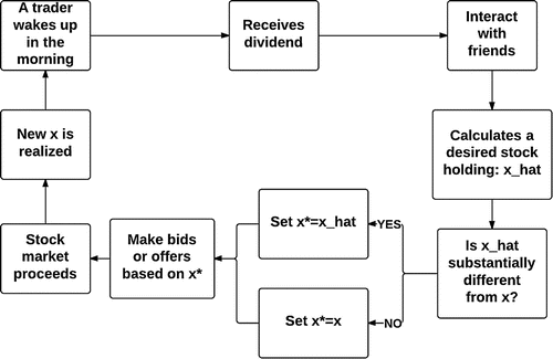
Figure 1 depicts a typical day in the life of a trader. A trader starts out his day by receiving the dividend. Afterward, he goes out for interacting with his friends. From these mutual interactions, traders get informed of the current portfolio profiles of his friends. The profiles simply contain the stock holdings of his friends. After that, a trader reads through his all financial accounts and newspapers to collect relevant information for a subsequent trading. The information set, $I_{\mathit{it}}$, includes the portfolio profiles of neighboring traders (${\mathbf{X}}_t^{Z_i}$), the current number of stock shares ($S_{\mathit{it}}$), the current number of bonds ($B_{\mathit{it}}$), the stock price of a previous trading period ($P_t$), the current wealth ($W_{\mathit{it}}$),the bond price ($Q_t$), and dividend ($d_{t+1}$).⁶

Once a stock market opens up for trading, a trader i computes his desired stock holding, which is measured as a percentage of his current wealth. We assume the trader’s desired stock holding as a function of three distinct factors in the information set previously collected: the portfolio profiles of neighborhood; firm’s profitability; and past stock return performance. A trader may have a different weight on each factor, depending on his nature, experiences, etc. Consequently, for each trader, the weights placed on three factors determine his trading type. These weights will constitute important treatment factors which will be systematically varied in the subsequent computational experiments.

Once a trader determines his desired stock holding, he forms his demand bid or supply offer for stock shares and submits this bid/offer to the stock market. Afterward, stock bids/offers are matched to achieve a market clearing solution consisting of a trading volume and a closing stock price. Subsequently, his new stock holding ($x_{\mathit{it}}$), which is defined as a ratio of the cash value of shares to wealth, is realized. This step finalizes one day of a trader. In the model, all traders go through this daily routine. In the following subsections, we provide the detailed explanations for each component in the routine. Tables 1 and 2 can be used for references in the following discussions.

Table 1. Summary of endogenous variables

List endogenous variables
Description	Admissibility conditions
Number of bonds	$B_{\mathit{it}}\in {\mathbf{R}}_{+}$
Stock price	$P_t$
Stock return	$r_t=\frac{P_t-P_{t-1}}{P_{t-1}}$
Number of stock shares	$S_{\mathit{it}}\in {\mathbf{R}}_{+}$
Realized portfolio weight on stock	$x_{\mathit{it}}=\frac{P_t{S}_{\mathit{it}}}{P_t{S}_{\mathit{it}}+Q_t{B}_{\mathit{it}}}\in [0,1]$
Temporary desired portfolio weight on stock	${\widehat{x}}_{\mathit{it}}\in [0,1]$
Final desired portfolio weight on stock	$x_{\mathit{it}}^{\ast }\in [0,1]$
Portfolio weights of neighborhood	${\mathbf{X}}_t^{Z_i}={\{x_{\mathit{jt}}\}}_{j\in Z_i}$
Wealth	$W_{\mathit{it}}$

Table 2. Summary of exogenous variables

Exogenous variables
Description	Admissibility conditions
Weights on neighborhood	${\mathbf{a}}_i^{Z_i}={\{a_{\mathit{ij}}\}}_{j\in Z_i}\text{s.t.}{\sum }_{j=1}^{N_i}{a}_{\mathit{ij}}=1$
Dividend	$d_t$
Moving average of dividend	${\overline{d}}_t^{h_i}=({\sum }_{k=t-h_i}^t{d}_k)/h_i$
Memory length	$h_i<\infty$
Total number of traders in the market	$N\in {\mathbf{R}}_{+}$
Number of traders in neighborhood	$N_i=|Z_i|$
Price of bonds	$Q_t=\frac{1}{r_f}$
Risk-free rate	$r_f\in [0,1]$
Tolerance level	$To{l}_i\in [0,1]$
Set of interacting traders	$Z_i$
Weight on network factor	${\mathit{\alpha }}_i\in [0,1]$
Weight on dividend factor	${\mathit{\beta }}_i\in [0,1]$
Aggression parameter of dividend factor	${\mathit{\gamma }}_i^f\in {\mathbf{R}}_{+}$
Aggression parameter of technical factor	${\mathit{\gamma }}_i^g\in {\mathbf{R}}_{+}$
Stochastic shock on the dividend	${\mathit{ϵ}}_t\sim N(0,1)$

2.2. Dividend payout

As described above, a trader starts out his day by receiving dividends for stock shares currently held. One notable assumption on dividend payments is that they are automatically converted to the risk-free bonds before submitting a bid or an offer for stock shares. This assumption is pivotal for the overall market dynamics because the dividend payments function as persistent disturbances in the current portfolio position of a trader, which may lead him to adjust his portfolio continuously.

We assume the logarithm of the dividend ($d_t$) follows a random walk with a drift ($\overline{d}$):(1) $$\begin{array}{c}\hfill log(d_t)=log(d_{t-1})+\overline{d}+\mathit{\sigma }{\mathit{ϵ}}_t\end{array}$$(1)

where $\mathit{\sigma }$ affects a volatility of the dividend process, and ${\mathit{ϵ}}_t$ is a Gaussian white noise term. Once the current dividend is paid out to the trader, it is recorded in the information set $I_{\mathit{it}}$ of trader i for subsequent use in portfolio rebalancing.

2.3. Social interaction

Figure 2. The network structure of traders.

Note: This figure illustrates how 100 traders are linked. Note that each node represents a single trader.

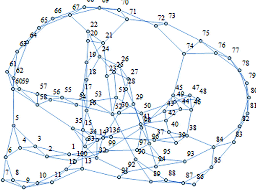
As mentioned in the introduction, the salient feature of the model in this study is the existence of mutual interactions among traders that affect stock holdings in every trading period. The network structure, which defines a channel through which the interactions among traders occur, is one of the crucial features of the model. In this study, we incorporate a Small-World Network (henceforth, SWN) as the network structure that I impose. The SWN is an extension of locally connected networks with a small number of traders having distant links to other traders in different local networks. It has been emerging as a good description of a realistic social network structure and has been widely applied in different contexts.⁷

Figure 2 illustrates how the social network among traders is structured in the model. Each node represents an individual trader. An edge which connects two nodes implies that two traders are linked. If traders are linked, they both affect each other in portfolio rebalancing. Let T denote the set of all traders in the market. Formally, the set $Z_i\in T$ is defined as follows.(2) $$\begin{array}{c}\hfill Z_i=\{j|q_{\mathit{ij}}=1,\forall j\in T\}\end{array}$$(2)

where $q_{\mathit{ij}}=1$ if i and j are linked. Otherwise, $q_{\mathit{ij}}=0$.The network structure assumed here is an undirected graph in which the direction of a link is not of importance. Formally, we can express the network structure as a symmetric matrix. I assume trader i regards himself as an element of $Z_i$. Therefore, all diagonal elements are one in a matrix representation of the network.

The interaction yields the portfolio profiles of neighborhood traders (${\mathbf{X}}_t^{Z_i}$), a vector of stock holdings of traders in interactions. The portfolio profiles for the traders in $Z_i$ are assumed to be included in the information set for trader i.

2.4. Desired stock holding

In rational expectation asset pricing models, the optimal portfolio weight can be easily computed using only the expected return and volatility of an asset.⁸ Unlike this conventional approach, we rather exploit behavioral assumptions that enable us to embrace a higher degree of heterogeneity. The factors included in the model need not be restricted to the specific factors used in the current study.

In this stock market model, the key process in the daily routine of a trader is how a trader calculates his provisional⁹ desired stock holding as a percentage of his wealth, at the beginning of the period. As will be clarified below, we assume that the provisional desired stock holding (${\widehat{x}}_{it+1}$) of a trader i is a function of three factors: firm profitability; a past stock return; and the investment behavior of other traders. These factors are called as “dividend factor,” “technical factor,” and “network factor,” respectively.

The dividend factor enters into a trader’s consideration as a signal for a firm’s future profitability. A trader takes into account of the relative profitability of the firm, which is expressed as a deviation of the current dividend from a moving average of past dividends. This factor influences an agent’s decision as follows: a positive deviation of from the moving average signals traders to increase their stock holding, and vice versa.

The technical factor is the stock return ($r_t$)¹⁰ realized in the previous trading period. Specifically, we assume the positive stock return in the previous trading period causes the trader to rebalance his portfolio in favor of stocks over bonds. This type of behavioral pattern has been ascribed to momentum traders in the computational literature or leveraged financial institutions with risk regulations.¹¹

The network factor, which is a byproduct of interactions, gets traders infused with a beauty contest environment that leads them to mimic the behavior of other traders in their neighborhood sets. For example, if one trader finds that weighted average of stock holdings in his networking boundary has increased, then (all else equal) he will rebalance his portfolio in favor of more stocks.

Summing up, the provisional desired stock holding (${\widehat{x}}_{i,t+1}$) for period $t+1$ is specifically determined as follows:(3) $$\begin{array}{c}\hfill {\widehat{x}}_{i,t+1}={[{\mathbf{a}}_i{\mathbf{x}}_t^{Z_i}]}^{{\mathit{\alpha }}_i}{\left[f\left(\frac{d_t-{\overline{d}}_t^{h_i}}{{\overline{d}}_t^{h_i}}\right)\right]}^{{\mathit{\beta }}_i}{[g(r_t)]}^{1-{\mathit{\alpha }}_i-\mathit{\beta }i}\end{array}$$(3)

where ${\mathbf{a}}_i$ is a vector of weights on the portfolio profiles of neighboring traders, ${\overline{d}}_t^{h_i}$ is an $h_i$ period’s moving average of dividend, ${\mathit{\alpha }}_i$ is a weight on the network factor and ${\mathit{\beta }}_i$ is a weight on the dividend factor. The memory length, $h_i$, of a trader i determines the extent of past dividend data usage in forming the dividend moving average. This parameter is one of the key variables of the model. For example, a higher value of memory length implies the use of longer time series of dividend in computing the dividend moving average. As will be seen, the dynamics of stock market depend strongly on the choice of $h_i$. A high degree of trader heterogeneity can be implemented by varying the weights $({\mathit{\alpha }}_i,{\mathit{\beta }}_i)$ assigned to the network factor and dividend factor for each trader i. Depending on the values of these weights, a trader can be categorized as one of the following four trading types:

Definition 1

A trader i is a “dividend trader” iff ${\mathit{\alpha }}_i=0,{\mathit{\beta }}_i=1$.

Definition 2

A trader i is a “technical trader” iff ${\mathit{\alpha }}_i=0,{\mathit{\beta }}_i=0$.

Definition 3

A trader i is a “network trader” iff ${\mathit{\alpha }}_i=1,{\mathit{\beta }}_i=0$.

Definition 4

A trader i is a “hybrid trader” iff ${\mathit{\alpha }}_i\in (0,1),{\mathit{\beta }}_i\in (0,1)$.

The functional forms of f and g in (3(3) $$\begin{array}{c}\hfill {\widehat{x}}_{i,t+1}={[{\mathbf{a}}_i{\mathbf{x}}_t^{Z_i}]}^{{\mathit{\alpha }}_i}{\left[f\left(\frac{d_t-{\overline{d}}_t^{h_i}}{{\overline{d}}_t^{h_i}}\right)\right]}^{{\mathit{\beta }}_i}{[g(r_t)]}^{1-{\mathit{\alpha }}_i-\mathit{\beta }i}\end{array}$$(3) ) are given by (4(4) $$\begin{array}{c}\hfill f(z)=\frac{1}{1+exp(-{\mathit{\gamma }}_i^{f}z)}\end{array}$$(4) ) and (5(5) $$\begin{array}{c}\hfill g(z)=\frac{1}{1+exp(-{\mathit{\gamma }}_i^{g}z)}\end{array}$$(5) ):(4) $$\begin{array}{c}\hfill f(z)=\frac{1}{1+exp(-{\mathit{\gamma }}_i^{f}z)}\end{array}$$(4) (5) $$\begin{array}{c}\hfill g(z)=\frac{1}{1+exp(-{\mathit{\gamma }}_i^{g}z)}\end{array}$$(5)

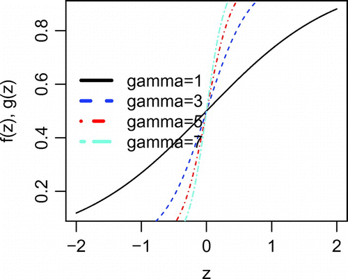
where ${\mathit{\gamma }}_i^f$ is an aggression parameter for the dividend factor and ${\mathit{\gamma }}_i^g$ is an aggression parameter for the stock return factor. In other words, the functions f, g are response functions which determine how aggressively a trader reacts to innovations in the dividend factor and the stock return factor. These response functions map the real line onto the open unit interval (i.e. $f,g:R\to (0,1)$) in a monotonically increasing manner. Figure 3 illustrates how the curvatures of f and g change with changes in the aggression parameters (${\mathit{\gamma }}_i^f$, ${\mathit{\gamma }}_i^g$).

Figure 3. Effects of changes in the agression parameters ${\mathit{\gamma }}^f$ and ${\mathit{\gamma }}^g$ on the curvatures of f(z) and g(z).

2.5. Systemic inertia

After computing the provisional desired stock holding (${\widehat{x}}_{i,t+1}$) for period $t+1$, a trader i’s next task in period t is to determine the final desired stock holding ($x_{i,t+1}^{\ast }$). We assume that the desired stock holding changes only if the provisional desired stock holding (${\widehat{x}}_{i,t+1}$) deviates significantly from the current stock holding ($x_{\mathit{it}}$).

Specifically, it is modeled by introducing the systemic inertia into the portfolio rebalancing: a tolerance level ($To{l}_i$) of a trader i acts as a proxy for this inertia, which dampens the possibility of frequent trading.¹² By this construction, we infuse the model with the additional source of heterogeneity.¹³

The final desired stock holding ($x_{i,t+1}^{\ast }$), which will be the basis for a bid or an offer for stock shares, is determined as follows:(6) $$\begin{array}{c}\hfill x_{i,t+1}^{\ast }=\left\{\begin{array}{cc}{x}_{i,t}\hfill & ,\text{if}|{\widehat{x}}_{i,t+1}-x_{i,t}|\le To{l}_i\hfill \\ {\widehat{x}}_{i,t+1}\hfill & ,\text{otherwise}\hfill \end{array}\right.\end{array}$$(6)

Note that (6(6) $$\begin{array}{c}\hfill x_{i,t+1}^{\ast }=\left\{\begin{array}{cc}{x}_{i,t}\hfill & ,\text{if}|{\widehat{x}}_{i,t+1}-x_{i,t}|\le To{l}_i\hfill \\ {\widehat{x}}_{i,t+1}\hfill & ,\text{otherwise}\hfill \end{array}\right.\end{array}$$(6) ) prevents frantic trading behavior in the sense that it dampens the frequency of the desire to trade further.

2.6. Endogenous switching between buying and selling

Given a desired stock holding $x_{i,t+1}^{\ast }$ for period $t+1$, a trader i’s next task is to translate this desired stock holding into the number of shares using the prevailing stock price:(7) $$\begin{array}{c}\hfill S_{\mathit{it}}^{\ast }(P_{t+1})=\frac{W_{\mathit{it}}{x}_{i,t+1}^{\ast }}{P_{t+1}}\end{array}$$(7)

Subsequently, given $S_{i,t+1}^{\ast }$, a trader forms his demand or supply of stocks according to the following rule:(8) $$\begin{array}{c}\hfill \mathrm{\Delta }{S}_{\mathit{it}}^{\ast }(P_{t+1})=\frac{W_{\mathit{it}}{x}_{i,t+1}^{\ast }}{P_{t+1}}-S_{\mathit{it}}\end{array}$$(8)

Let ${\mathit{\varphi }}_{i,t+1}$ be an index for trading direction at the beginning of trading period $t+1$. Let ${\mathit{\varphi }}_{i,t+1}=1$ if a trader wishes to buy, and let ${\mathit{\varphi }}_{i,t+1}=-1$ if trader i wishes to sell. Otherwise, let ${\mathit{\varphi }}_{i,t+1}=0$. Then it follows that(9) $$\begin{array}{c}\hfill {\mathit{\varphi }}_{i,t+1}=\left\{\begin{array}{cc}1\hfill & \text{if}\mathrm{\Delta }{S}_{\mathit{it}}^{\ast }(P_{t+1})>0\hfill \\ -1\hfill & \text{if}\mathrm{\Delta }{S}_{\mathit{it}}^{\ast }(P_{t+1})<0\hfill \\ 0\hfill & \text{if}\mathrm{\Delta }{S}_{\mathit{it}}^{\ast }(P_{t+1})=0\hfill \end{array}\right.\end{array}$$(9)

Equation (9(9) $$\begin{array}{c}\hfill {\mathit{\varphi }}_{i,t+1}=\left\{\begin{array}{cc}1\hfill & \text{if}\mathrm{\Delta }{S}_{\mathit{it}}^{\ast }(P_{t+1})>0\hfill \\ -1\hfill & \text{if}\mathrm{\Delta }{S}_{\mathit{it}}^{\ast }(P_{t+1})<0\hfill \\ 0\hfill & \text{if}\mathrm{\Delta }{S}_{\mathit{it}}^{\ast }(P_{t+1})=0\hfill \end{array}\right.\end{array}$$(9) ) implies that a trader has a unique switching price ($P_{i,t+1}^s$) at which his trading direction changes. We can easily observe that the heterogeneity in the switching price is the definitive source of exchanges for stock shares. For instance, if all traders collapse to the same switching price, the no-trade state emerges.

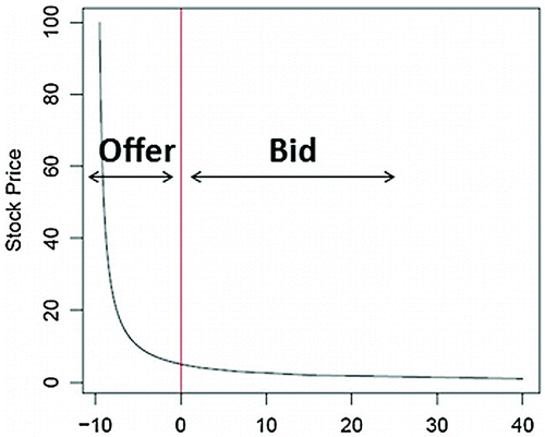
Figure 4 shows how the demand or the supply for stock changes with variations in the stock price. The left side of the red vertical line denotes the selling domain, while the right side of this line denotes the buying domain. It demonstrates that the trading direction of a trader is endogenously determined by the prevailing stock price.

Figure 4. Bid/offer curve of a trader.

Note: The depicted curve is the graph of $\mathrm{\Delta }{S}_{\mathit{it}}^{\ast }(P)$ as a function of stock price P. Trader i switches his trading position at the point where the curve and the vertical line intersect.

2.7. Market price determination

In this study, it is assumed that there is a Walrasian auctioneer who adjusts the stock price to clear the market using a tâtonnement process. When the auctioneer announces a stock price, traders make bids or offers by the announced price. The auctioneer then adjusts the stock price until the stock market clears. However, we restrict an increment in the tâtonnement process to be unity, which implies that the market price cannot be infinitely finetuned to clear the market. Therefore, in this setting, there is no guarantee that the market clearing stock price exists. If it does not exist, the auctioneer closes the trading period with the unique price that minimizes excess demand or excess supply as follows:(10) $$\begin{array}{c}\hfill P_{t+1}^{\ast }:=argmin\sum _i\mathrm{\Delta }{S}_{\mathit{it}}^{\ast }(P_{t+1})\end{array}$$(10)

The rationale for this restriction is to achieve a reconciliation between the ideal Walrasian equilibrium world and the real stock market that is frequently characterized by uncleared bids and offers in the order book. If there are uncleared bids or offers, a rationing is executed randomly. For an excess demand (supply) case, the rationing of stock shares is put into effect only for buyers (sellers). Given this rationing scheme, a trader may end up being only partially successful in achieving the desired portfolio rebalancing.

3. Experimental design

3.1. Specification of treatment parameter values

The model is quite flexible in terms of allowing investigation of market dynamics under various settings. To demonstrate it as a flexible platform, we consider six simple cases as clear illustrations of the proposed model. One treatment factor varied across these cases is memory length ($h_i$)¹⁴ upon which the dividend moving average is computed: short-memory length (i.e. ten trading periods) vs. long-memory length (i.e. one hundred trading periods). Two additional treatment factors varied across these cases are the weight ${\mathit{\alpha }}_i$ on the network factor and the weight ${\mathit{\beta }}_i$ on the dividend factor in the determination of the provisional desired stock holdings ${\widehat{x}}_{i,t+1}^{\ast }$ for each trader i; see (3(3) $$\begin{array}{c}\hfill {\widehat{x}}_{i,t+1}={[{\mathbf{a}}_i{\mathbf{x}}_t^{Z_i}]}^{{\mathit{\alpha }}_i}{\left[f\left(\frac{d_t-{\overline{d}}_t^{h_i}}{{\overline{d}}_t^{h_i}}\right)\right]}^{{\mathit{\beta }}_i}{[g(r_t)]}^{1-{\mathit{\alpha }}_i-\mathit{\beta }i}\end{array}$$(3) ).

Table 3 lists the six cases studied in our simulation experiments. Since exploring all possible pairs of values for $\mathit{\alpha }$ and $\mathit{\beta }$ is prohibitive, we restrict our analysis to three pure types of traders who consider only one factor in the determination of their provisional desired stock holdings (${\mathit{\alpha }}_i=0$ or ${\mathit{\beta }}_i=0$) and one hybrid trader type who places equal weight on all three factors in the determination of his provisional desired stock holdings (${\mathit{\alpha }}_i={\mathit{\beta }}_i=1/3$).

Table 3. Six cases to be experimentally studied

Case number	Type description	${\mathit{\alpha }}_i$	${\mathit{\beta }}_i$	$h_i$
1	long-memory dividend trader	0	1	100
2	short-memory dividend trader	0	1	10
3	Technical trader	0	0	n.a.
4	Network trader	1	0	n.a.
5	long-memory hybrid trader	1/3	1/3	100
6	short-memory hybrid trader	1/3	1/3	10

Notes: The network and technical trader cases do not involve a data truncation issue. Hence, a varying degree of memory length ($h_i$) is not considered for these cases.

3.2. Specification for maintained parameter values

In this section, we provide the specific values of exogenous variables for which each case in Table 3 is implemented. Table 4 lists values of exogenous variables used in this study.

The dividend process (1(1) $$\begin{array}{c}\hfill log(d_t)=log(d_{t-1})+\overline{d}+\mathit{\sigma }{\mathit{ϵ}}_t\end{array}$$(1) ) is calibrated to Shiller’s monthly real dividend data¹⁵, yielding $\overline{d}=0.0014$, $\mathit{\sigma }=0.0072$. The number of traders (N) in this stock market model is an important dimension we have to consider. Given that a very small number of traders would give a low chance of having the diversity in the market, we set the total number of traders to be 100. We find that this is a reasonable number that allows the model to have enough diversity regarding distributions of wealth, the number of stock shares, and the number of risk-free bonds. At the initialization step, the initial endowment $S_{i0}$ and $B_{i0}$ of stocks and bonds for each trader i are drawn from uniform distributions, $S_{i0}\sim \text{Uniform}(S_L,S_U)$, $B_{i0}\sim \text{Uniform}(B_L,B_U)$.

For simplicity, the return on the risk-free bond ($r_f$) is exogenously given as 0%. We assume there is no upper bound for the total supply of risk-free bonds. Also, we assume the weights (${\mathit{\alpha }}_i$, ${\mathit{\beta }}_i$) on factors are all equal across hybrid traders. A tolerance level ($To{l}_i$) is randomly drawn for each trader from a uniform distribution bounded between $To{l}_L$ and $To{l}_U$. We set memory length to be ten trading periods for the short-memory case and 100 trading periods for the long-memory case.¹⁶ For the network factor, we assume, for simplicity, that a trader weighs equally the portfolio profiles of his neighborhood traders, which means each neighborhood trader’s stock holding gets a weight of $1/N_i$. The ranges of tested values for the three trader attributes (${\mathit{\alpha }}_i$,${\mathit{\beta }}_i$) selected as treatments factors are given in Table 3.

Table 4. Maintained parameter values

Parameters	Values
Number of traders (N)	100
Risk-free rate ($r_f$)	0
Aggression parameter for dividend factor (${\mathit{\gamma }}_i^f$)	5
Aggression parameter for technical factor (${\mathit{\gamma }}_i^g$)	5
Initial stock price ($P_0$)	166
Initial dividend ($d_0$)	10
Long-memory length ($h_i^{\mathit{long}}$)	100
Short-memory length ($h_i^{\mathit{short}}$)	10
Drift in the dividend process ($\overline{d}$)	0.0014
Volatility of the dividend process ($\mathit{\sigma }$)	0.0072
Lower bound of initial stock number ($S_L$)	0
Upper bound of initial stock number ($S_U$)	100
Lower bound of initial bond number ($B_L$)	0
Upper bound of initial bond number ($B_U$)	100
Lower bound of tolerance level ($To{l}_L$)	0
Upper bound of tolerance level ($To{l}_U$)	0.1
Neighborhood weights (${\mathbf{a}}_i$)	$(\frac{1}{N_i},\frac{1}{N_i},\cdots ,\frac{1}{N_i},\frac{1}{N_i})$

Notes: The neighborhood weights vary by trader since a trader’s number of links to other traders is heterogeneous. A trader i’s initial numbers of stocks and bonds will be maintained throughout all test cases.

4. Simulation results

In this section, we present the simulated stock market dynamics in which only a single type of traders exists.¹⁷ The stock market dynamics along with the statistical properties of stock returns will be presented for each case, and comparisons between the cases will be made. Even though the stock market with the single type of traders seems to be unrealistic, these experiments would provide a general picture of how the stock market evolves and would serve as benchmarks on which extensions could be developed for future studies.

4.1. Case 1 and Case 2: Dividend trader

For the dividend trader cases, we divide them into two subcases depending on memory length: long-memory vs. short-memory. The simulated times series for key endogenous variables for the dividend trader cases are shown in Figures 5 and 6. In those figures, the top panels show the simulated series of stock prices and the middle panels show the simulated stock returns series. Finally, the bottom panels exhibit the series of trading volumes.

In both cases, the stock prices tend to trace out an upward trend in the dividend process, while the stock market with long-memory dividend traders generates more volatile stock price fluctuations. At first glance, this seems to stand in sharp contrast with the intuition: more use of the historical data creates higher stock return volatilities.

However, this is a natural consequence of the stochastic process of the dividend. As specified previously, the dividend process follows a random walk with a positive drift. Given that the dividend moving average based on the long-memory length moves slower than the short-memory length in response to the new realization of the dividend in the current period, it is highly likely that the currently realized dividend differs much greater from the moving average in the long-memory case.

This greater discrepancy creates more rooms for the portfolio rebalancing. In other words, given that dividend follows a non-stationary process, the dividend moving average based on the long-memory scheme is prone to being irrelevant for evaluating the current profitability of the firm. Therefore, comparing the current dividend level to the long-memory moving average solicits more reactions from traders. This might cause more jagged fluctuations in stock prices.

The simulated moments of stock returns for the dividend trader cases are presented in Table 5. The stock return distributions are characterized by being leptokurtic given that the excessive kurtosis is positive for two dividend trader cases, suggesting the existence of fat-tail in the stock return distributions. The table also shows that the long-memory case exhibits a greater dispersion in the stock return distribution than the short-memory case.

Comparing the simulated moments to those of the dividend process, both the long-memory dividend trader case and short-memory dividend trader case exhibit the excessive volatility and fat tail properties observed in actual stock return data, while the first moments are similar to the drift in the dividend process. These results, indeed, are in line with Shiller ’s (1981) empirical observations.

To check the existence of conditional heteroscedasticity in stock return volatility, we carry out ARCH effect tests proposed by Engle (1982). The test rejects the null hypothesis that there are no ARCH effects in stock return volatilities. Table 6 presents LM test statistics for various lags. F-statistics of these tests are highly significant, with p-values being close to zero, for all lags considered.

Figure 5. Stock market dynamics: Long-memory dividend trader (Case 1).

The horizontal x-axis denotes trading periods.

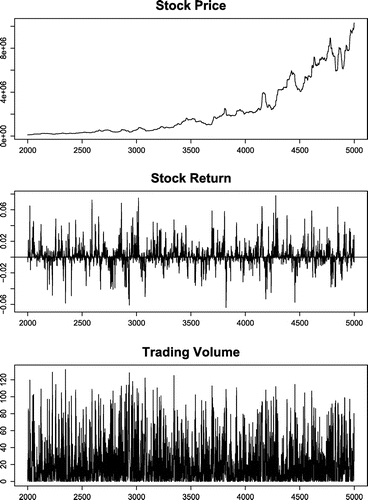
Figure 6. Stock market dynamics: Short-memory dividend trader (Case 2).

The horizontal x-axis denotes trading periods.

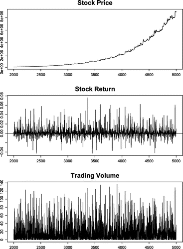
Table 5. Summary of stock return statistical properties: Dividend traders

	1st moment	2nd moment	Skewness	Excessive Kurtosis
Long-memory	0.0015	0.0127	0.5885	5.7744
	(0.0001)	(0.0006)	(0.1863)	(0.779)
Short-memory	0.0015	0.0099	1.4434	8.5657
	(0.0001)	(0.0003)	(0.2097)	(1.4881)

Notes: Values in parentheses denote standard deviation from 1,000 runs under the calibrated dividend process. Excessive kurtosis is defined as the fourth moment of a distribution less the fourth moment of a standard normal distribution.

Table 6. ARCH effect tests for stock returns: Dividend traders

	$l=1$	$l=2$	$l=3$	$l=4$	$l=5$	$l=6$
Long-memory	606.3	310	214.6	163.1	130.6	108.8
	(2.2e-16)	(2.2e-16)	(2.2e-16)	(2.2e-16)	(2.2e-16)	(2.2e-16)
Short-memory	79.8	40.91	27.3	20.75	16.72	14.1
	(2.2e-16)	(2.2e-16)	(2.2e-16)	(2.2e-16)	(2.535e-16)	(6.753e-16)

Note: Estimates are F-statistics of LM tests proposed by Engle (1982). Values in parentheses denote p-values of F-statistics of LM tests. Notice that l denotes a number of lags in each test.

4.2. Case 3: Technical traders

As a next pure type trader, we report the simulation results for runs of the stock market populated only with technical traders. In this run, all traders are heterogeneous in terms of their initial endowments and levels.¹⁸

Technical traders anchor on the stock return in rebalancing their portfolios. Regarding the memory length, technical traders have super-short-memory lengths in the sense that the stock returns in other periods do not matter, except for the previous trading period. By construction, technical traders inject positive feedback into stock prices for they demand more stock shares after a large stock price increase, and conversely.

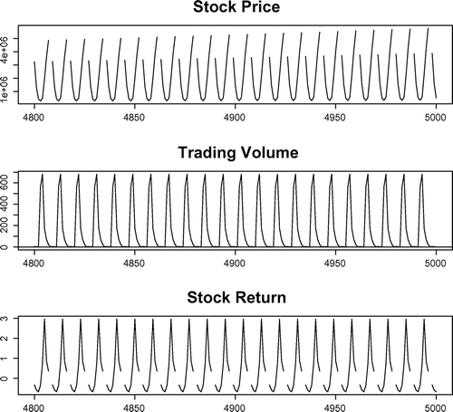
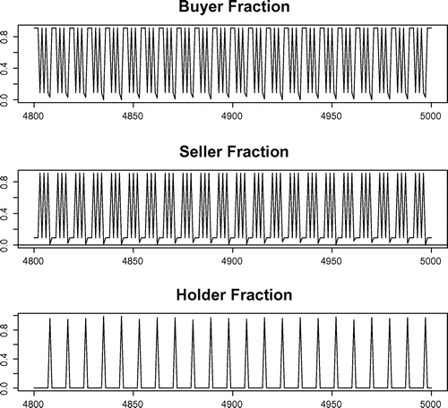
Figure 7 shows the simulated series of key variables of the stock market with technical traders. The top panel shows the simulated stock price series, which exhibits a quite stable cyclical pattern with an upward trend. The upward trend seems to reflect the wealth effect generated by the periodic dividend payments.¹⁹ One notable finding, in this case, is the collapse in stock prices following no-trade states in each cycle.²⁰

Investigating the volume of trading shows that cyclical ups and downs in stock prices accompany with the same pattern of trading volume. The trading volume and the stock price fluctuations are highly correlated in this case. As shown in Figure 8, the stock market is marked by the frequent dominance of one type of market forces.

At this point, we have to ask what triggers the collapse in stock prices and make exchanges resume after no-trade states. It is intuitively unclear about this cyclical pattern. However, the detailed investigation of simulated data provides us with the clue about this cyclical pattern. The peak in stock prices is always followed by the no-trade states. In principle, the no-trade state leads to the indeterminacy of a stock price in that period. As construction, we assume that traders evaluate, during no-trade states, their wealth based the stock price in the period followed by the no-trade period.²¹ In addition to that, we further assume that technical traders perceive stock returns in the no-trade state periods as zero. This leads to the greater difference between the current portfolio and the desired portfolio in the periods following no-trade periods.²²

Figure 7. Stock market dynamics: Technical trader (Case 3).

The horizontal x-axis denotes trading periods. The disconnected portions of plots denote the periods in which no trades occur.

Figure 8. Trading profile: Technical trader (Case 3).

The horizontal x-axis denotes trading periods.

4.3. Case 4: Network traders

The other intriguing component of the model is that it captures the mimetic behavior of a trader by incorporating the neighborhood portfolio profile into the portfolio choice of a trader. In this section, we report simulation findings from runs of the stock market model with network traders linked under SWN.

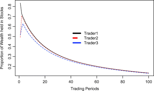
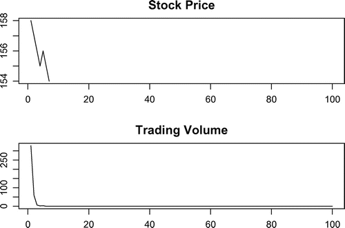
The top panel of Figure 9 shows the simulated stock prices during the first 100 trading periods. After a few of adjustment periods, the stock prices stay constant as no-trade states continue. The simulated trading volume series is presented in the bottom panel of Figure 9. It suggests that the difference between a trader’s portfolio weight and his neighborhoods’ portfolio weights quickly disappear by the initial rounds of stock exchanges. This can be verified in Figure 10, which shows the time paths of $x_{\mathit{it}}$ for three traders in the run. Trader 1 and Trader 2 are directly linked, while Trader 3 has no direct links with two other traders. Traders 1 and Trader 2 end up with the similar level of portfolio weights after one trading period. On the other hand, Trader 3 remains still below that level. A downward trend in $x_{\mathit{it}}$ for all trader is due to the subsequent no-trade states and the continuous dividend payments in the form of risk-free bonds.

It is interesting to observe that trades do not resume even after dividend payment. This may happen because, once a pure-network trader conforms his portfolio weight to those of his neighboring traders, he will not engage in further trades unless the dividend payments disturb his wealth in a way that makes $x_{\mathit{it}}$ deviate significantly from the average stock shareholdings of his neighborhood traders. Since traders must be outside their tolerance levels before they change their current stock holdings, the small perturbations caused by dividend payments do not result in further trades.

Even though the stock market populated with network traders produces simple results, we expect the role of network traders would not be negligible for the stock market in which network traders interact with other types of traders. Mimicking other traders’ investment behavior might give rise to complex market dynamics. For example, suppose the stock market is populated with dividend traders (i.e. fundamentalists) and network traders. Even small perturbations to the fundamentals can lead to overreaction (De Bondt & Thaler, 1985) in asset prices due to herd behavior by network traders, which implies mimicking behavior can become a key destabilizing factor in financial markets.²³

Figure 9. Stock market dynamics: Network trader (Case 4).

The horizontal x-axis denotes trading periods.

Figure 10. Stock holding comparison between network traders.

4.3.1. Case 5 and Case 6: Hybrid trader cases

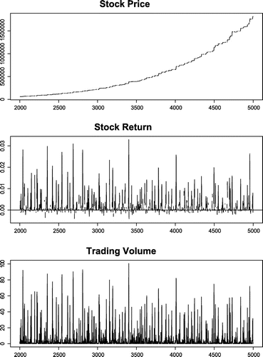
In this section, we report results from the cases in which traders consider all three factors. As in the dividend trader cases, we also have two experiment environments depending on memory length: long-memory length vs. short-memory length. The simulated run of the stock market with the long-memory hybrid traders is presented in Figure 11, and that of stock market with short-memory hybrid traders is shown in Figure 12. In those figures, the top panels show simulated stock prices and the middle panels show simulated stock returns. The bottom panels show the simulated volume of trade. Table 7 summarizes the moments of the simulated stock returns. Unlike the dividend trader case, there is not a substantial difference in the second moments between the two cases, while the fat tail property is more pronounced in the long-memory case.

The simulated moments of stock returns, shown in Table 7, conform to the first moment and the second moment of the dividend process, while the third moment and the fourth moment are not consistent with a normal distribution. Comparing these hybrid trader cases to dividend trader cases, the stock market with hybrid traders seems to generate a less volatile stock return process.

As done in dividend trader cases, we also conduct ARCH effect tests for stock returns generated in hybrid trader cases. We reject the null hypothesis that there are no ARCH effects in stock return volatilities. Table 8 shows that F-statistics of these tests are highly significant for all lags considered.

Figure 11. Stock market dynamics: long-memory hybrid trader (Case 5).

The horizontal x-axis denotes trading periods.

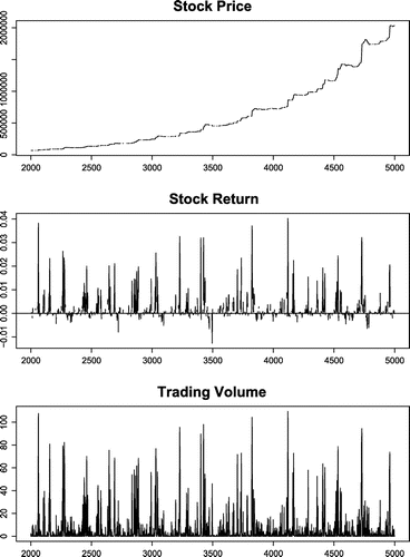
Table 7. Summary of stock return statistical properties: Hybrid traders ARCH effect tests for stock returns: Hybrid traders

	1st moment	2nd moment	Skewness	Excessive Kurtosis
Long-memory	0.0014	0.0062	4.9082	31.5835
	(0.0001)	(0.0004)	(0.47)01	(6.3364)
Short-memory	0.0017	0.0064	4.7670	28.8932
	(0.0001)	(0.0004)	(0.3735)	(5.3781)

Notes: Values in parentheses denote standard deviation from 1,000 runs under calibrated dividend process. Excessive kurtosis is defined as the fourth moment of a distribution less the fourth moment of a standard normal distribution.

Table 8. ARCH effect tests for stock returns: Hybrid traders

	$l=1$	$l=2$	$l=3$	$l=4$	$l=5$	$l=6$
Long-memory	3,991	3,224	2,358	1,785	1,427	1,189
	(2.2e-16)	(2.2e-16)	(2.2e-16)	(2.2e-16)	(2.2e-16)	(2.2e-16)
Short-memory	2,575	1,943	1,434	1,102	883.3	736.1
	(2.2e-16)	(2.2e-16)	(2.2e-16)	(2.2e-16)	(2.2e-16)	(2.2e-16)

Notes: Estimates are F-statistics of LM tests proposed by Engle (1982). Values in parentheses denote p-values of F-statistics of LM tests. Notice that l denotes a number of lags in each test.

4.4. Post-earnings shock dynamics

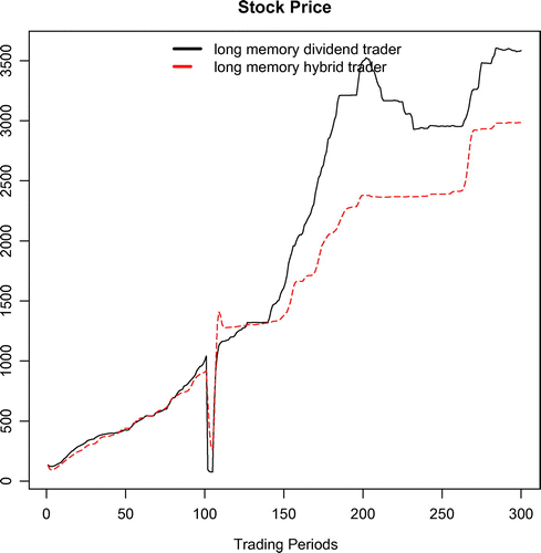
In this section, we investigate how earnings shocks leading to periods, when no dividends are paid, affects the stock price dynamics. In these experiments, the only difference is made on the dividend process: We construct an experimental environment in which the firm goes through a recession, which forces it not to make dividend payments to shareholders for four trading periods. Specifically, negative earnings shocks begin at time t = 100 and continue until t = 103, referred to below as the recessionary phase. The dividend process then reverts to its normal path, referred to below as the recovery phase.

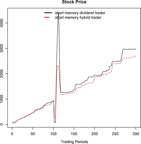
Figure 13 compares stock price fluctuations between the long-memory dividend trader case and the long-memory hybrid trader case. It shows that, for the long-memory hybrid trader case, the stock price falls to a lesser extent than the long-memory dividend trader case. The interesting finding is that stock prices overshoot to a greater extent during the recovery phase from the recession. This implies the long-memory hybrid trader case generates an asymmetry in stock prices between the recessionary phase and the expansionary phase.

The stock price asymmetry in response to shocks can be explained by interactions between the washing-out effect and the positive-feedback effect, both of which are caused by the technical factor and the network factor in ${\widehat{x}}_{\mathit{it}}$. It seems that the washing-out effect dominates the stock price dynamics at the beginning of the recessionary phase, while the positive-feedback effect dominates the stock price dynamics during the recovery phase. The sources of these two effects are the same, but the timings of occurrence differ. At the beginning of the recessionary phase, traders have a strong desire to sell stock shares because their current zero dividend deviates significantly from the dividend moving average. On the contrary, at the recovery phase, other factors amplify the urge to buy more shares, which eventually leads to overshooting in stock prices.

The short-memory case is presented in Figure 14. As opposed to the long-memory case, the overshooting in stock prices is more pronounced for the short-memory dividend trader case. This finding implies that the dramatic innovation in earnings in the recovery phase gets more amplified in the short-memory dividend trader case. This is because earnings performance in the recession periods dominates in the moving average based on short-memory compared to those in relatively distant periods.

Figure 12. Stock market dynamics: Short-memory hybrid trader (Case 6).

The horizontal x-axis denotes trading periods.

Figure 13. Recovery phase dynamics: Long-memory sases.

Figure 14. Recovery phase dynamics: Short-memory cases.

4.5. Wealth dynamics

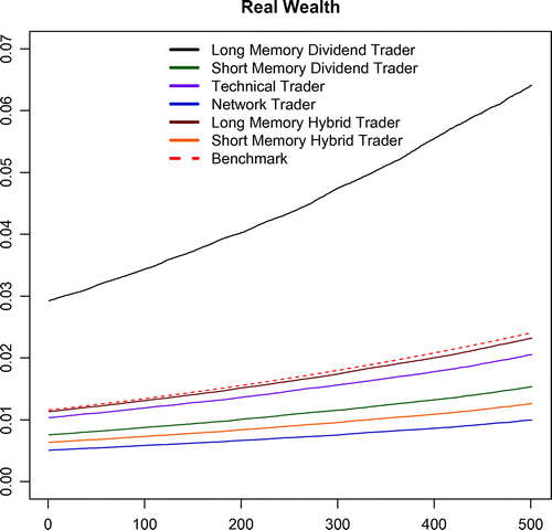
In this section, we consider the real wealth²⁴ dynamics across different trading types. In this experiment, we populate the stock market with multiple trading types. Note that traders are structurally same except trading type and tolerance level parameter ($To{l}_i$). Let $Avg{M}_t^r$ denote the cross-sectional average real wealth of traders of a specific trading type in period t for the rth run of the simulation. ²⁵ Figure shows, depending the trading type, an average real wealth of traders ($Avg{M}_t$), which is averaged across multiple runs in each period. ²⁶

According to Figure 15, the long memory dividend traders’ average wealth is highest among six types of traders, while network traders most underperform. Table 9 presents the average wealth growth rate of each trading type. Regarding wealth growth, we don’t observe any discernible differences among different trading types except that technical traders’ wealth growth exhibits the highest volatility.

There is a caveat to making inferences from the results in Figure 15: it is inappropriate to conclude that one trading type is superior to other types by simply observing these results. To check the supremacy of one strategy to others, we have to introduce an evolutionary market environment in which the composition of traders is dynamically changing according to some performance measures.

In other words, it is closely related to the question of whether switching from one trading type to another trading type yields a higher wealth growth, while all other traders are also simultaneously contemplating possible moves. In this environment, a stock market is inherently dynamic. Thus, the superiority of one trading type should be investigated in a context that permits a dynamically changing composition of traders.²⁷

Figure 15. Average wealth by trading type (AvgMt).

Figures are based on 100 simulation runs. The benchmark denotes the average wealth in which stock shares are equally distributed to all traders and no trades occur. Note that real wealth levels are normalized by a constant number for easier illustrations.

My future research will focus on the possibility of the emergence of a stable composition of trading types, including the possible dominance of one trading type.

Table 9. Growth rate of average wealth

	Mean (%)	Standard deviation (%)
Long-memory Diviend Trader	0.15	0.07
Short-memory Diviend Trader	0.14	0.07
Technical Trader	0.13	0.12
Network Trader	0.13	0.09
Long-memory Hybrid Trader	0.14	0.07
Short-memory Hybrid Trader	0.13	0.07

Note: These estimates are based on 100 simulation runs. In each run, the growth rate of average wealth is based on $Avg{M}_r^t)$, and the initial 2,000 observations are discarded to eliminate the effects of initial conditions; i.e. Mean = $\left({\sum }_{r=1}^{N_r}{\sum }_{t=2001}^T\frac{\mathrm{\Delta }Avg{M}_t^r}{Avg{M}_{t-1}^r}\right)/(N_r+3000)$ where $N_r$ = 100 and T = 5000.

5. Concluding remarks

This study develops a simple yet flexible stock market model permitting the comparative study of different types of stock trading behaviors about market performance. Certain types of behaviors have been shown to result in stock return outcomes matching the stylized facts of actual stock markets.

Depending on the choice of information set²⁸ from which traders anchor for portfolio rebalancing, traders are modeled into three different trading types: dividend trader, technical trader, and network trader.²⁹ Furthermore, the endogenous trading decision of buying and selling, coupled with a stock rationing scheme in case of the nonexistence of a market clearing price, is another distinguishing feature of the model.

This study shows that stock market performance metrics are quite sensitive to the trading types of traders and memory length. Specifically, if all traders only consider the firm dividend, and the dividend process is non-stationary, then long-memory traders make the stock return process more volatile than short-memory traders. If all traders only consider a past stock return, stock prices exhibit a cyclical pattern. On the other hand, if all traders simply mimic the choices of their neighborhood traders, the stock market converges to a no-trade state after short periods of stock exchanges. Finally, the fat-tailed property in the distribution of stock returns is more pronounced when traders place equal weight on the three factors than when traders place weight only on firm profitability.

The model is subject to several limitations. First of all, the feature of no learning capabilities is unrealistic in the sense that real-world agents make constant adaptations to the ever-changing environment. For example, when the market consists only of pure technical traders, who only consider a past stock return movement, there is a possibility to exploit the resulting clear pattern in stock prices.

One possible way to overcome this limitation is to introduce learning algorithms for the formation of weights on the three factors. Specifically, instead of assuming fixed weights on the factors determining trading behavior, traders could learn how to set these weight by some performance measures. This type of extension opens the door to capturing both heterogeneity and the adaptive behavior of traders.

The other limitation of the model is the fact that, unlike traditional risk-based asset pricing models, the model does not take into account the risk preferences of traders. To introduce a volatility measure as one of the factors would be an effective way of overcoming this limitation. Additionally, a different measure of firm profitability, such as dividend yield, could be used, provided the stylized fact that dividend yield predicts future asset returns for several asset classes (Cochrane, 1993).

Various interesting extensions of this work can be undertaken. First, this stock market model can be appropriately embedded into a macroeconomic model in which the dividend of a firm is endogenously determined by the firm’s innovation endeavor. Second, the stock market model can be generalized to permit different types of traders to compete for survival. It would be interesting to see whether particular types of trading eventually dominate the market in this evolutionary setting. Third, allowing traders to choose their trade networks endogenously is another intriguing application. This extension would make it possible to explore how the stock market dynamics and the network properties are inter-related and coevolve. Finally, the study on stock market performance from competition between rational fundamental traders and behavioral traders described in the model would be an additional contributing factor to the Efficient Market Hypothesis debate.

Additional information

Funding

The author received no direct funding for this research.

Notes on contributors

Dong-Jin Pyo

Dong-Jin Pyo is a financial economist at the Financial Supervisory Service. His research interests include agent-based computational modeling of financial markets, the interactions between financial sector and the macroeconomy, and the application of big data analytics to financial markets.

Notes

Current affiliation: Macroeconomics and Finance Research Team, Financial Supervisory Service, Address: 38 Yeoui-Daero, Youngdeungpo-Gu, Seoul, Korea.

1 The prototype of agent-based artificial stock market can be found in Arthur et al. (1997). For studies on adaptive behavior based on genetic algorithms in asset market context, see Arifovic (1996), Chen and Yeh (2001), Kluger and McBride (2011), and Arthur, LeBaron and Palmer (1999). Endogenous switching between different forecasting rules are considered in numerous models, such as Brock and Hommes (1998), Lux and Marchesi (2005), and Chiarella and He (2002).

2 The idea of network effects dates back to Keynes ’s (1936) beauty contest metaphor for stock market investment. The modeling approach adopted here does not exactly coincide with the concept of Keynes’s beauty contest. This study rather focuses on the mimicking behavior of traders, while the beauty contest emphasizes the importance of higher order belief among market participants

3 This type of modeling approach is similarly implemented in Thurner, Farmer and Geanakoplos (2009).

4 We regard knowing the fundamental price of a stock share as being incompatible with the imperfect knowledge of the actual data generating process that determines firm’s fundamental value.

5 Analyses on the indirect mimetic behavior of traders in the context of computational stock markets are found in Lux (1998) and Iori (2002). Iori (2002) develops a multi-agent stock market model under which trading decision depends on communication between traders and idiosyncratic shocks. She identifies that the imitating behavior and trading frictions are key elements of volatility clustering. Compared to Iori (2002), Lux (1998) develops a model in which mimetic behavior is implemented in a less direct sense. In this model, conversion between optimistic chartist and pessimistic chartist is stochastically executed through a global variable, i.e. an opinion index.

6 Note that all of the trader subsequent actions are conditional on this information set. The notation for an information set of a trader i will be suppressed in the following sections for notational simplicity.

7 For the extensive survey of network analyses in economic contexts, see Jackson (2008). For a brief introduction to the Small-World Network, see Watts and Strogatz (1998). For application to bilateral trading, see Wilhite (2001).

8 In other words, the coordination among agents is made only through global variables.

9 As shown in Figure , the final desired stock holding will be determined in a subsequent step.

10 As in the financial literature, the stock return is defined to exclude dividend payments. This is usually done since dividend payments are irregular. For modeling purposes, this is to capture a pure price movement impact on the demand of a trader.

11 A price increase in a risky asset leaves additional room for capital buffers, which leads to more purchases of a risky asset. For more details, see Shin (2010).

12 Although trading frictions are not explicitly modeled in this study, the introduction of a tolerance level implicitly brings a similar effect of having trading frictions prevalent in the market.

13 We checked that the presence of heterogeneity in the threshold level is a key source of market liquidity. Even when the only structural differences among traders are their tolerance levels, we observed that exchanges among traders occur.

14 For the definition of $h_i$, see Section 2.4.

15 http://www.econ.yale.edu/shiller/data.htm. Data from 1950:1-2012:12 are used.

16 A heterogeneous memory length is a very critical aspect of the asset market dynamics. For simplicity, this study does not consider heterogeneous memory length or evolutionary learning algorithms. This topic would deserve a separate future study. For interested readers , refer to LeBaron (2001a, b, 2012), and Mitra (2005).

17 Note all traders are characterized by the same specification of weights on factors for each case. Refer to Table 3.

18 As in the dividend trader case, we observed that the heterogeneity in the tolerance level solely could generate stock exchanges among traders. And it should be noted that initial conditions are identical across different cases except trading styles.

19 In a run with the dividend being zero during all periods, we found that the upward trend vanishes, and the market collapses to the no-trading state after a few periods of active exchanges.

20 The no-trade states are marked by the discontinuous portion in the figure.

21 This pricing rule is arbitrary, and the market dynamics will depend on the specific pricing rule in no-trade states. The simple pricing rule adopted in this study prevents a complete explosion or a bust in stock prices during relatively short periods in case of the stock market with technical traders

22 The no-trade state poses delicate issues which have rarely been dealt within the earlier computational stock market models. The existing asset pricing models systemically exclude the occurrence of no-trade states since it is assumed that there is always a fixed number of stock shares supplied.

23 Herd behavior may arise from either cognitive biases (e.g. availability bias) or rational responses to uncertainty. Herd behavior can easily occur because, in a highly connected society, a peer group often provides a channel for easily accessible and recallable information on which people can rely. On the other hand, the latter case is related to the notion of information cascade in which an agent follows previous actions made by other agents, ignoring his private signal (i.e. Banerjee (1992), Bikhchandani, Hirshleifer, & Welch (1992)).

24 In this simulation, the real wealth refers to individual trader’s cash balance after each trading period.

25 Note that $Avg{M}_t^r={\sum }_i^{100}{M}_{\mathit{it}}^r/100$ where $M_{\mathit{it}}^r$ is individual trader i’s real wealth in period t for the rth run.

26 $Avg{M}_t={\sum }_r^{N_r}Avg{M}_t^r/N_r$ where $N_r$ is the number of simulation runs.

27 In this context, LeBaron (2001a) delivers a counterargument against Friedman’s natural selection hypothesis by reminding us that the population of the market itself is dynamically changing. He raises the question of “who is rational” in “what sense“: “In Friedman’s world, rational traders have started off rational world. So the small infusion of irrational traders doesn’t alter the whole picture of the market. But if we start the market off in another way such as market dominated by short-memory traders, the story would be reversed."

28 The full information set consists of three distinct elements: dividend as a measure for firm profitability, past stock return movements, and imitation of neighborhood traders, all of which are shown to be important in many empirical studies. See Section 2.4 for references for the studies which shows the significance of these factors.

29 See Section 2.4 for the exact definitions of trading types.

References

- Arifovic, J. (1996). The behavior of the exchange rate in the genetic algorithm and experimental economies. Journal of Political Economy, 104(3), 510–541.
- Arthur, W. B., LeBaron, B., Palmer, R., & Tayler, P. (1997). Asset pricing under endogenous expectations in an artificial stock market in The Economy as an Evolving Complex system 2. Brian Arthur, W., Durlauf, S. & Lane, D. eds. Addison-Wesley.
- Arthur, W. B., LeBaron, B., & Palmer, R. (1999). Time series properties of an artificial stock market. Journal of Economic Dynamics and Control, 23(9), 1487–1516.
- Banerjee, A. V. (1992). A simple model of herd behavior. The Quarterly Journal of Economics, 107(3), 797–817.
- Bikhchandani, S., Hirshleifer, D., & Welch, I. (1992). A theory of fads, fashion, custom, and cultural change as information cascades. Journal of Political Economy, 100(5), 992–1026.
- Brock, W. A., & Hommes, Cars H. (1998). Heterogeneous beliefs and routes to chaos in a simple asset pricing model. Journal of Economic Dynamics and Control, 22(8), 1235–1274.
- Brown, J. R., Ivković, Z., Smith, P. A., & Weisbenner, S. (2008). Neighbors matter: Causal community effects and stock market participation. The Journal of Finance, 63(3), 1509–1531.
- Chen, S.-H., & Yeh, C.-H. (2001). Evolving traders and the business school with genetic programming: A new architecture of the agent-based artificial stock market. Journal of Economic Dynamics and Control, 25(3), 363–393.
- Chiarella, C., & He, X.-Z. (2002). Heterogeneous beliefs, risk and learning in a simple asset pricing model. Computational Economics, 19(1), 95–132.
- Chiarella, C., Iori, G., & Perelló, J. (2009). The impact of heterogeneous trading rules on the limit order book and order flows. Journal of Economic Dynamics and Control, 33(3), 525–537.
- Cochrane, J. H. (1993). Discount rates. The. Journal of Finance, 66(4), 1047–1108.
- De Bondt, W., & Thaler, R. (1985). Does the stock market overreact? The Journal of Finance, 40(3), 7930–805.
- Engle, R. (1982). Autoregressive conditional heteroscedasticity with estimates of the variance of United Kingdom inflation. Econometrica, 50(4), 987–1007.
- Hong, H., Kubik, J. D., & Stein, J. C. (2004). Social interaction and stock-market participation. The Journal of Finance, 59(1), 137–163.
- Hong, H., Kubik, J. D., & Stein, J. C. (2005). Thy neighbor’s portfolio: Word-of-mouth effects in the holdings and trades of money managers. The Journal of Finance, 60(6), 2801–2824.
- Iori, G. (2002). A microsimulation of traders activity in the stock market: The role of heterogeneity, agents’ interactions and trade frictions. Journal of Economic Behavior & Organization, 49(2), 269–285.
- Jackson, M. O. (2008). Social and Economic Networks. New Jersey: Princeton University Press.
- Keynes, J. M. (1936). The General Theory of Employment. Harcourt, Brace and World, New York: Interest and Money.
- Kluger, B. D., & McBride, M. E. (2011). Intraday trading patterns in an intelligent autonomous agent-based stock market. Journal of Economic Behavior & Organization, 79(3), 226–245.
- LeBaron, B. (2001a). Evolution and time horizons in an agent-based stock market. Macroeconomic Dynamics, 5(2), 225–254.
- LeBaron, B. (2001b). Calibrating an agent-based financial market to macroeconomic time series. mimeo, Brandeis University.
- LeBaron, B. (2012). Heterogeneous gain learning and the dynamics of asset prices. Journal of Economic Behavior & Organization, 83(3), 424–445.
- Lux, T. (1998). The socio-economic dynamics of speculative markets: Interacting agents, chaos, and the fat tails of return distributions. Journal of Economic Behavior & Organization, 33(2), 143–165.
- Lux, T., & Marchesi, M. (2005). Volatility clustering in financial markets: A microsimulation of interacting agents. International Journal of Theoretical and Applied Finance, 3(4), 675–702.
- Malloy, C., Frazzini, A., & Cohen, L. (2008). The small world of investing: Board connections and mutual fund returns. Journal of Political Economy, 116(5), 951–979.
- Mitra, K. (2005). Is more data better? Journal of Economic Behavior & Organization, 56(2), 263–273.
- Shiller, R., & Pound, J. (1989). Survey evidence on diffusion of interest and information among investors. Journal of Economic Behavior & Organization, 12(1), 47–66.
- Shiller, R. J. (1981). Do stock prices move too much to be justified by subsequent changes in dividends? American Economic Review, 71(3), 421–436.
- Shin, H. S. (2010). Risk and liquidity. Oxford: Oxford University Press.
- Thurner, S., Farmer, D., & Geanakoplos, J. (2009). Leverage causes fat tails and clustered volatility. Quantitative Finance, 12(5), 695–707.
- Watts, D. J., & Strogatz, S. H. (1998). Collective dynamics of ‘Small-World’ networks. Nature, 393, 440–442.
- Wilhite, A. (2001). Bilateral trade and ‘Small-World’ networks. Computational Economics, 18(1), 49–64.