Could pension system make us happier?

Abstract

This paper analyzes the effect of public pension system on lifespan and happiness level using optimal longevity model. This paper found the following. Public pension system can make life expectancy longer, however, the extension of lifespan caused by the public pension, not by own decision, cannot make happiness level higher. Under the government budget constraint, the public pension system cannot make the happiness level higher comparing to private savings. This paper concludes that the compulsory public pension system should be reconsidered because it does not contribute to well-being but raises various problems like aging population and income inequality.

Keywords:

• optimized life expectancy
• lifetime utility level
• health investments
• public pension system
• private savings

AMS Subject Classifications:

• C61
• H55
• I31

Public Interest Statement

A serious issue of many countries is expected to be an aged income guarantee system because of the public pension exhaustion and aging population. According to Melbourne Mercer Global Pension Index, US, Germany, France, UK, Italy, etc., their pension systems have major risks and/or shortcomings that should be addressed. Without improvements, its efficacy and/or long-term sustainability can be questioned. This research deals with very interesting questions whether the sheer existence of a public pension system makes people happier and live longer. This research found the following. Public pension system can increase life expectancy; however, the extension of lifespan caused by the public pension, not by own decision, cannot increase the level of happiness. The public pension system cannot increase the level of happiness if compared with private savings. Public pension systems don’t contribute to well-being, but raise various problems like aging population and income inequality and therefore should be reconsidered.

1. Introduction

Believe it or not, according to an anecdote in Europe, as soon as a pension system was introduced, the number of people who jog in the park for their health increased. If we have a pension system, it looks like a good deal, if we live long enough to enjoy in pension. This research analyzes the effect of a pension system on life expectancy and happiness level. Especially, this research will offer answers to the following questions. Could pension system make us happier? Could pension system make our lifespan longer? Is it always true that longevity ensures happiness? Which one is better, we plan our own future by ourselves or we rely on government pension system? and so on.

There are many literatures on the effect of rising longevity or health status on some economic variables as saving rate, growth rate, labor market, education, human capital accumulation, and so on.¹ Recently, Pestieau and Ponthiere (2012) surveys the various contributions to the impact of changes in longevity on various public policies. In many previous researches, the longevity or health status are the cause of the change in economic variables, which means the various changes of economic variables are the effects of the change caused by longevity or health status. However, there are few researches (e.g. Deaton, 2003; Philipson & Becker, 1998 etc.) in the opposite direction, that is, how economic variables, except income per capita, affect life expectancy or health. This research is different from previous researches in the fact that a pension system is the cause, and the life expectancy and the happiness level are its effects.

A vast amount of empirical and theoretical researches about the economic welfare of a pension system has been accumulated. The main results of some previous studies on pension system and economic welfare can be summarized as follows: under a fully funded system, the economic welfare is not affected; however, under a pay-as-you-go (PAYG) pension system, depending on the economic situations and generations, the economic welfare might be both improved or worsened. The public pension system as a risk-hedging device can increase welfare by providing a certainty in the imperfect market (e.g. Bohn, 2009; Krueger & Kubler, 2002; Sánchez-Marcos & Sánchez-Martin, 2006; Shiller, 1999, etc.). The compulsory pension system which is one of the forced saving policies can lead to high saving rates, meanwhile, the public pension system crowds out the private savings. The pension system can have a negative effect on the capital accumulation and can retard growth (e.g. Cutler & Gruber, 1996; Feldstein & Liebman, 2002, etc.). If the public pension system does not crowd out the private savings, the public pension system which is a compulsory saving can raise the national saving rate and the growth rate. The overall welfare impact depends on the balance between the insurance effect and the crowding-out effect. This research shows that the public pension system has both positive and negative effect on welfare; however, under government budget constraint, it is difficult that the public pension system improves welfare level even though the pension system has an insurance effect which makes the risk of uncertainty lower.

There are two general ways to study on longevity in theory, which are overlapping generation model and optimal dynamic model. Many previous researches use the overlapping generation models, (e.g. Pecchenino and Pollard (1997), Chakraborty (2004), Momota et al. (2005), Sánchez-Marcos and Sánchez-Martin (2006), Ponthiere (2009), etc.). In many previous overlapping generation models, the maximum lifespan has been given (e.g. two-period or three-period) and the survival probability has been introduced and the life expectancy has been calculated by the average of the longevity of the people who live to the maximum lifespan and the people who die before the maximum lifespan depending on the survival probability. Actually, in two-period model, only two kinds of ages (i.e. one-period-old and two-period-old) exist and nobody survives more than the given period even though the life expectancy has variations. Meanwhile, some previous researches use the optimal dynamic models (e.g. Dalgaard & Strulik, 2014; Ehrlich & Chuma , Ehrlich; Grossman, 1972, etc.). The idea that the individual’s longevity is based from the result of the individual’s utility maximization problem is the same with both models, but in the optimal dynamic models, the individual decides about the time when he/she will die, at the terminal point of the continuous time model, to maximize his/her happiness level. This research paper has followed the latter.

We use an optimal dynamic problem of individuals who live in continuous time to analyze the effect of a pension system on life expectancy and happiness level. We develop a simple life cycle model in which the length of life is endogenously determined by individual’s optimal health investments. Our model is primarily related to Ehrlich and Chuma (1990) and Dalgaard and Strulik (2014) which apply optimal longevity. We have simplified Dalgaard and Strulik (2014) and introduced a pension system into it. We consider that the individual’s longevity is based from the result of the individual’s utility maximization problem. Individuals could choose to live a short and intensely happy life, or a longer and less intensely happy life, or a moderate long and moderate happy life.² If the length of life is chosen optimally, the relationship of the length of life and the level of happiness could not be proportional because there is a trade-off between the quantity and quality of life. We consider a lifetime utility maximization problem between the length of life and the level of happiness under individual’s budget constraint. An individual distributes his/her budget to his/her basic needs and to his/her health investments to maximize his/her lifetime utility. Along with Grossman (1972) which models optimal health investment in increasing longevity, we assumed that it is possible to extend lifespan by the effort of an individual through health investments.³ We suggested two kinds of method to hedge against an uncertainty in life which are public pension model and private savings model. In the public pension model, an individual pays his/her pension to government mandatorily when he/she is young and the individual gets his/her pension when he/she becomes old which continues until his/her death. In the private savings model, an individual saves an extra money for an extended period in which he/she could be still alive unexpectedly even though the money may go to waste if he/she dies earlier unexpectedly. Whichever method he/she chooses between two methods, he/she does not have to worry about financing future years of living.

We have investigated how the optimized lifespan and the lifetime utility level have been changed by the existence or non-existence of the pension system. We have compared the lifetime utility level of the public pension model as a compulsory saving with the lifetime utility level of the private savings model as voluntary saving. We have shown following three important results using this research model: (1) Pension system can make the lifespan longer. This result is consistent with Philipson and Becker (1998) which argued that there is a moral hazard effect in public pension that induces excessive longevity. The pension system can rather raise problems for aging population which affect the country’s productivity and growth rate negatively through the decline in the fraction of working-age population. (2) Under government budget constraint, even though public pension can make the lifespan longer, the public pension cannot make the happiness level higher comparing to the private savings. The public pension as a compulsory saving can distort individual’s decision and make the individual worse off. If the prediction of lifespan does not turn out to be completely wrong under lifetime uncertainty, it is not always true that the pension system improves the lifetime utility level even though the pension system has an insurance effect or a risk-hedging function. (3) Generally, life expectancy itself is proportional to the happiness; however, life expectancy may not be always proportional to happiness unless income support accompanies. The extension of lifespan caused by the public pension cannot make our happiness level higher. The extension of lifespan only chosen by own decision and accompanied by the income support may make our happiness higher. Furthermore, we have formulated and tested three hypotheses based on the results of theoretical model. We have shown that three results roughly correspond to the characteristics of cross country data.

This research, I believe, is the first one to provide the empirical evidence for the first result which has been argued by Philipson & Becker (1998). Furthermore, both, the second and the third results, are discussed theoretically and empirically for the first time using the optimal longevity model and the cross country data. These results suggest that the compulsory public pension system should be reconsidered because it does not contribute to well-being but raises various problems like aging population and income inequality.

This paper is organized as follows: Section 2 presents a benchmark model and solves the model numerically. Section 3 introduces an uncertainty in the benchmark model and deals with two risk-hedge models and analyzes the results. Section 4 tests the results from the theoretical models empirically using cross country data. Section 5 offers conclusions on this research. Finally, more information on each country and the detailed calculation can be found in Appendix.

2. The benchmark model

In this section, we have created a benchmark model which is an utility maximization model to analyze the relationship between the life expectancy and the level of happiness. And in the following section, we will introduce a pension system into the benchmark model to analyze the relationship between the existence or non-existence of a pension system and the life expectancy and the relationship between the existence or non-existence of a pension system and the level of happiness. Frey (2008) mentioned that the lifetime utility is used to measure the level of happiness which is an abstract variable. Happiness is not exactly the same with utility, but both happiness and utility have a close relationship and the higher the utility level is, the higher the happiness level is. We assume that happiness is a way of measuring utility.⁴

2.1. Setup

Grossman (1972) developed a model on demand for health through health investments. After that, Ehrlich and Chuma (1990) developed a model of demand function for longevity and derived optimal longevity and time path for health capital, health investment, and consumption. Dalgaard and Strulik (2014) introduced the low of motion which governs the aging process to the optimal longevity model and elaborated it. The benchmark model is primarily related to Ehrlich and Chuma (1990) and Dalgaard and Strulik (2014) which consider on health investments and optimal longevity. We consider an individual’s utility maximization problem under the finite period. He/She can live up to T years old and die at the age of T. There is no uncertainty in the model and individuals have perfect foresight. We will introduce an uncertainty in lifetime in Section 3. An individual maximizes his/her lifetime utility which is affected by consumption. The instantaneous utility function $(u(·))$ is specified in log form as follows:(1) $$\begin{array}{c}\hfill u(c)=lnc\end{array}$$(1)

where c is consumption. We think that it is possible to extend the lifespan by the efforts of the individual. We assume that there is a linear relationship between health investment and the lifespan as follows:(2) $$\begin{array}{c}\hfill T=a+bz,(a>0,b>0),\end{array}$$(2)

where T and z are the lifespan and the health investment, respectively. And a and b are positive constants. When z is decided, T is automatically decided, on the contrary, when T is decided, z is automatically decided, which means if we invest amount of z, we can live until T and if we want to live until T, we should invest amount of z. If an individual invests for his/her health more, as the result, his/her lifespan will be longer. The lifespan T is finite and endogenous. Grossman (1972) and Ehrlich and Chuma (1990) introduced state of health in utility function named as stock of health and amount of healthy time, respectively. However, we assume that the health investments do not affect the utility directly like Philipson and Becker (1998) and Dalgaard and Strulik (2014).⁵ Dalgaard and Strulik (2014) introduced Mitnitski and Rockwood’s equation which measures how human frailty and proportion of deficits increase as humans get older to express the physiological relationship between aging and mortality. For simplification, we did not use Mitnitski and Rockwood’s equation which is a non-linear function. We also assume that the interest earning is the only source of income of the individual, and there is no labor income and no production division.⁶ And to simplify, a small open country is assumed, then the domestic interest rate is always constant. We denote the individual’s asset as x, then his/her budget constraint is written as follows:(3) $$\begin{array}{c}\hfill \dot{x}=rx-c-z,\end{array}$$(3)

where r is interest rate. We put the initial asset which the individual has as $x(0)=x_0$.

The individual’s utility maximization problem can be written as follows:(4) $$\begin{array}{cc}\hfill \underset{c(t),z}{max}{\int }_0^T{e}^{-\rho t}& lnc(t)dt,(0<\rho <1)\hfill \\ \hfill \mathrm{s}.\mathrm{t}\dot{x}(t)& =rx(t)-c(t)-z,\hfill \\ \hfill T& =a+bz,\hfill \\ \hfill x(0)& =x_0,\hfill \end{array}$$(4)

where $\rho$ is discount rate. We assume the $\rho$ is constant, that is, this model is a exponential discounting model, not a hyperbolic discounting model which is treated in behavioral economics. We assume $r\ge \rho$.⁷ In many previous studies (e.g. Dalgaard & Strulik, 2014; Ehrlich & Chuma, 1990; Grossman, 1972, etc.), health state which is a accumulation of health investment is introduced as a state variable similar to human capital. However, for simplification, we assume that z has a constant value from the initial period until T period, $z(0)=\cdots =z(T)=z$, and that z is decided at the initial period. ⁸ Life expectancy is the number of years a person can expect to live in given social environments when he/she is born. We assume that when an individual is born, he/she decides how much he/she invests for his/her health and how long he/she lives in the social environments surrounding him/her which are $x_0$, a, b, r, $\rho$, etc.

2.2. Solving the Model

The maximization problem is solved in two stages. At the first stage, we consider that T and z in Equation (2) are given values, not control variables. At the second stage, we consider the T and z as control variables. First, we maximize over c and x for any given T and z, and then the objective function which has been maximized with respect to c and x could be described as a function of T and z. Second, we maximize over T and z instead of c and x, because c and x have been maximized in the first stage, that means c and x are a functions of time t, i.e. c(t|T, z) and x(t|T, z).

2.2.1. The First Stage

We use the Hamiltonian method to solve the maximization problem. The Hamiltonian is written as follows:(5) $$\begin{array}{c}\hfill H=lnc+\lambda (rx-c-z).\end{array}$$(5)

By differentiating Equation (5) with respect to c and x, we can get Equations (6) and (7).(6) $$\begin{array}{c}\hfill \frac{\partial H}{\partial c}=\frac{1}{c}-\lambda =0\Rightarrow c={\lambda }^{-1},\end{array}$$(6) (7) $$\begin{array}{c}\hfill \frac{\partial H}{\partial x}=\rho \lambda -\dot{\lambda }=\lambda r\Rightarrow \frac{\dot{\lambda }}{\lambda }=\rho -r.\end{array}$$(7)

We integrate Equation (7) to time t, then we get(8) $$\begin{array}{c}\hfill ln\lambda =(\rho -r)t+k\end{array}$$(8)

where k is a constant of integration. Taking exponential both sides of Equation (8), then we can get(9) $$\begin{array}{c}\hfill \lambda =C_1{e}^{(\rho -r)t},\end{array}$$(9)

where $C_1=e^k$. Substituting Equations (6) and (9) into Equation (3), we obtain the following(10) $$\begin{array}{c}\hfill \dot{x}-rx+z=-C_1^{-1}{e}^{-\rho t}{e}^{\mathit{rt}}.\end{array}$$(10)

This differential equation is solved as follows,(11) $$\begin{array}{c}\hfill x=\frac{1}{C_1}(\frac{e^{-\rho t}-1}{\rho })e^{\mathit{rt}}+C_2{e}^{\mathit{rt}}+\frac{z}{r}\end{array}$$(11)

where $C_2$ is a constant. See Appendix for the detailed calculation. $C_1$ and $C_2$ can be obtained from substituting the initial condition and transversality condition. Because of $x(0)=x_0$, we get $C_2$ as follows:(12) $$\begin{array}{c}\hfill C_2=x_0-\frac{z}{r}.\end{array}$$(12)

To maximize his/her utility, when dying, he/she uses up all his/her assets and leaves nothing. In other words, $x(T)=0$. We get $C_1$ as follows,(13) $$\begin{array}{c}\hfill C_1=\frac{1}{\rho }\frac{1-e^{-\rho T}}{x_0-(1-e^{-rT})\frac{z}{r}}.\end{array}$$(13)

Substituting Equations (12) and (13) into Equation (11), we obtain the following(14) $$\begin{array}{c}\hfill x(t)=\frac{x_0-(1-e^{-rT})\frac{z}{r}}{1-e^{-\rho T}}(e^{-\rho t}-1)e^{\mathit{rt}}+(x_0-\frac{z}{r})e^{\mathit{rt}}+\frac{z}{r}.\end{array}$$(14)

Substituting Equation (9) into Equation(6), we can get(15) $$\begin{array}{c}\hfill c(t)=\rho \frac{x_0-(1-e^{-rT})\frac{z}{r}}{1-e^{-\rho T}}{e}^{(r-\rho )t}.\end{array}$$(15)

Equations (14) and (15) are the optimal paths of x and c, respectively, in the situation where the variables T and z are fixed.

2.2.2. The Second Stage

In the second stage, to maximize his/her lifetime utility, the individual considers Equation (2) by choosing his/her optimal T. We can rewrite the utility maximization problem as follows:(16) $$\begin{array}{cc}\hfill \underset{T}{max}{\int }_0^T{e}^{-\rho t}& ln(\rho \frac{x_0-(1-e^{-rT})\frac{z}{r}}{1-e^{-\rho T}}{e}^{(r-\rho )t})dt\hfill \\ \hfill & \mathrm{s}.\mathrm{t}T=a+bz\hfill \end{array}$$(16)

We solve the integral in Equation (16), then we can induce Equation (17)(17) $$\begin{array}{c}\hfill {\int }_0^T{e}^{-\rho t}ln(\rho \frac{x_0-(1-e^{-rT})\frac{z}{r}}{1-e^{-\rho T}}{e}^{(r-\rho )t})dt=-ln(\rho \frac{x_0-(1-e^{-rT})\frac{z}{r}}{1-e^{-\rho T}})(\frac{e^{-\rho T}-1}{\rho })-(r-\rho )(\frac{(\rho T+1)e^{-\rho T}-1}{{\rho }^2}).\end{array}$$(17)

See Appendix for the detailed calculation. Substituting Equation (2) into Equation (17), the maximization problem can be rewritten as Equation (18) which has no integral and has only one control variable T. Equation (18) is just a static maximization problem, not a dynamic problem.(18) $$\begin{array}{c}\hfill \underset{T}{max}ln(\rho \frac{x_0-(1-e^{-rT})\frac{T-a}{\mathit{rb}}}{1-e^{-\rho T}})(\frac{1-e^{-\rho T}}{\rho })+(r-\rho )(\frac{1-(\rho T+1)e^{-\rho T}}{{\rho }^2}).\end{array}$$(18)

We take the derivative of Equation (18) with respect to T, then we can get(19) $$\begin{array}{c}\hfill f(T)=e^{-\rho T}ln(\rho \frac{x_0-(1-e^{-rT})\frac{T-a}{\mathit{br}}}{1-e^{-\rho T}})-\frac{1-e^{-\rho T}}{\rho b}\frac{e^{-rT}(T-a)+(1-e^{-rT})\frac{1}{r}}{x_0-(1-e^{-rT})\frac{T-a}{\mathit{br}}}-e^{-\rho T}+(r-\rho )T{e}^{-\rho T}.\end{array}$$(19)

By setting the first derivative to zero as $f(T|x_0,a,b,r,\rho )=0$, we can solve the utility maximization problem for T. In Ehrlich and Chuma (1990), the transversality conditions were considered. However, in this research model, we have considered the boundary conditions as Dalgaard and Strulik (2014), because the individual chooses T directly which is the terminal date.

2.3. Results

The implicit function $f(T|x_0,a,b,r,\rho )=0$ is highly non-linear, so it is difficult to solve it analytically. The alternative option is to provide the solutions numerically.⁹ The suitable parameter values are used for the calculation, though they are arbitrary. The parameter values that we use to calculate are the following: $a=20$, $b=10$, $x_0=100$, $\rho =0.01$, $r=0.02$. In order to investigate the effects of only the sheer pension system, not including the effect of income, we put the initial income as the constant value. We have obtained the optimal $T^{\ast }$ which is 24.556.¹⁰ We have put the optimal $T^{\ast }$ into Equation (18) and obtained the maximized $U^{\ast }$ which is 33.742. We have checked the convexity of Equation (18) in T numerically. ${\frac{{\partial }^{2}f(T)}{\partial T^2}}_{T=T^{\ast }}=-0.104$. The second derivative is negative, which means the function is concave if it is near the optimal $T^{\ast }$.¹¹

3. Lifetime uncertainty

Generally, we are prone to think that we have more need for survivor income programs which provided through the public sector (e.g. pensions, annuities) in case that we do not know, due to uncertainty, when we will die exactly. In Section 3, we consider an uncertainty in lifetime. We introduce an uncertainty in the T which individual chooses to maximize his/her lifetime utility. We add an uncertainty to Equation (2).(20) $$\begin{array}{c}\hfill T=a+bz+ϵ,\end{array}$$(20)

where $ϵ$ is a random variable with $E(ϵ)=0$ and symmetric distribution with respect to the mean, $-\varphi \le ϵ\le \varphi$, where $\varphi$ is a positive constant. When $ϵ$ is positive, an individual lives longer than the planned period T and when $ϵ$ is negative, an individual dies earlier than the planned period T.¹²$a+bz-\varphi \le T\le a+bz+\varphi$.

We suggest two methods to hedge against the uncertainty and to get income when an individual lives longer than the planned period T which are public pension and private savings. In the public pension model, an individual pays his/her pension to government mandatorily when he/she is young and the individual gets his/her pension when he/she becomes old which continues until his/her death. In the private savings model, an individual saves an extra money for an extended period in which he/she could be still alive unexpectedly even though the money may go to waste if he/she dies earlier unexpectedly. The individual can have stable resources in retirement due to two methods even though there is the uncertainty in life. We will compare both in order to determine which method is better.

3.1. Public pension

3.1.1. Setup

One of the purposes of this research is to analyze the effect of the pension system on the maximized utility and optimal longevity. We introduce a pension system into the benchmark model additionally. He/She pays a pension p from 0 to s period and gets a pension q after s period to death. The government decides about p, q,  and s which are constants as given to individuals. This pension system performs as a compulsory saving for individuals. The time from 0 to s is named as young period, while the time after s is named as old period. His/Her budget constraint in the benchmark model Equation (3) is changed to Equation (21).(21) $$\begin{array}{c}\hfill \dot{x}=\left\{\begin{array}{c}rx-c-z-p,\text{if}0\le t\le s(\mathrm{young}\mathrm{period})\hfill \\ rx-c-z+q,\text{if}s<t\le T(\mathrm{old}\mathrm{period}).\hfill \end{array}\right.\end{array}$$(21)

3.1.2. Solving the Model

Even though there is the uncertainty in life, he/she does not need to consider about the uncertainty, because if he/she lives longer than the planned period T, he/she will get the pension during positive $ϵ$. The way to solve the model with this pension system is similar to that of the benchmark model even though we have to divide it into young period and old period. Equation (11) is changed as follows:(22) $$\begin{array}{c}\hfill x=\left\{\begin{array}{c}\frac{1}{C_1^Y}(\frac{e^{-\rho t}-1}{\rho })e^{\mathit{rt}}+C_2^Y{e}^{\mathit{rt}}+\frac{z+p}{r},\text{if}0\le t\le s\hfill \\ \frac{1}{C_1^O}(\frac{e^{-\rho t}-1}{\rho })e^{\mathit{rt}}+C_2^O{e}^{\mathit{rt}}+\frac{z-q}{r},\text{if}s<t\le T.\hfill \end{array}\right.\end{array}$$(22)

where, $C_1^Y$, $C_2^Y$, $C_1^O,$ and $C_2^O$ are constants of integration which are as follows:(23) $$\begin{array}{c}\hfill C_1^Y=\frac{1}{\rho }\frac{1-e^{-\rho s}}{x_0-(1-e^{-rs})\frac{z+p}{r}-x(s)e^{-rs}}\end{array}$$(23) (24) $$\begin{array}{c}\hfill C_2^Y=x_0-\frac{z+p}{r}\end{array}$$(24) (25) $$\begin{array}{c}\hfill C_1^O=\frac{1}{\rho }\frac{(e^{-\rho T}-e^{-\rho s})e^{\mathit{rs}}}{\frac{z-q}{r}(1-e^{r(s-T)})-x(s)}\end{array}$$(25) (26) $$\begin{array}{c}\hfill C_2^O=\frac{\frac{z-q}{r}(1-e^{r(s-T)})-x(s)}{(e^{-\rho T}-e^{-\rho s})e^{\mathit{rs}}}(1-e^{-\rho T})-\frac{z-q}{r}{e}^{-rT},\end{array}$$(26)

where x(s) is interpreted as both the terminal value of young period and the initial value of old period at the same time.

By the same way as the previous, Equation (15) is changed as follows:(27) $$\begin{array}{c}\hfill c(t)=\left\{\begin{array}{c}\frac{1}{C_1^Y}{e}^{(r-\rho )t},\text{if}0\le t\le s\hfill \\ \frac{1}{C_1^O}{e}^{(r-\rho )t},\text{if}s<t\le T.\hfill \end{array}\right.\end{array}$$(27)

Substituting Equation (27) into the utility function, we have obtained the following(28) $$\begin{array}{c}\hfill {\int }_0^s{e}^{-\rho t}ln(\frac{1}{C_1^Y}{e}^{(r-\rho )t})dt+{\int }_s^T{e}^{-\rho t}ln(\frac{1}{C_1^O}{e}^{(r-\rho )t})dt\end{array}$$(28)

We integrate Equation (28) to time t, then we have gotten(29) $$\begin{array}{c}\hfill ln(\frac{1}{C_1^Y})\frac{1-e^{-\rho s}}{\rho }+ln(\frac{1}{C_1^O})\frac{e^{-\rho s}-e^{-\rho T}}{\rho }-(r-\rho )(\frac{(\rho T+1)e^{-\rho T}-1}{{\rho }^2}).\end{array}$$(29)

There are zs in $C_1^Y$, $C_2^Y$, $C_1^O$ and $C_2^O$. If we substitute $z=\frac{T-a}{b}$ into $C_1^Y$, $C_2^Y$, $C_1^O,$ and $C_2^O$, then, the original dynamic optimization problem with the pension system becomes static optimization problem with respect to T and x(s) as seen in Equation (30). In other words, all he/she has to do is to decide his/her own life expectancy and the initial asset at the old period.(30) $$\begin{array}{c}\hfill \underset{T,x(s)}{max}U(T,x(s))=ln(\frac{1}{C_1^Y(T,x(s))})\frac{1-e^{-\rho s}}{\rho }+ln(\frac{1}{C_1^O(T,x(s))})\frac{e^{-\rho s}-e^{-\rho T}}{\rho }-(r-\rho )(\frac{(\rho T+1)e^{-\rho T}-1}{{\rho }^2}).\end{array}$$(30)

3.1.3. Population structure and government budget

We assume that a certain big number of people with endowment $x_0$ is born in every period and that a, b, r, $\rho$ are constants, that is, the social environments surrounding individuals do not change over time.¹³ Because the individuals are born with same endowment, the optimized $T^{\ast }$s, which the individuals choose, are also same. Even though time will go, in the economy, the number of population will be the same and the population structure will not change.¹⁴ The period-by-period budget constraints of government are given as follows:(31) $$\begin{array}{c}\hfill \underset{\mathrm{revenue}}{\underbrace{\mathit{sp}}}=\underset{\mathrm{expenditure}}{\underbrace{(T-s)q}}.\end{array}$$(31)

The government collects p from each individual between the age of 0 and s and gives q to each individual between the age of s and T. The government collects sp from the young generation and pays $(T-s)q$ to the old generation. It can be a pay-as-you-go (PAYG) pension system. Because the population structure does not change, the government’s budget constraint holds Equation (31) in every period. Because $E(ϵ)=0$, the expected longevity is $E(T)=a+bz$. Someone dies before T-year-old and someone continues to live more than T. If there are lots of individuals in economy, the number of individuals who continue to live more than T will be equal to the number of individuals who die before T, because the random variable $ϵ$ is symmetric with respect to zero. By law of large numbers, the amount of pension which is paid to the individual T years of age or older can be covered from the amount of pension which is collected from the individuals who die younger than T.

3.1.4. Results

3.1.4.1. Grid search

Taking the derivative of Equation (30) with respect to T and x(s), and setting each first derivatives to zero, and solving the system of equations, we could obtain the optimal $T^{\ast }$ and $x{(s)}^{\ast }$. Since the object function of Equation (30) is highly non-linear and nested structure, it is very difficult to get an exact analytical solution for this problem. The alternative option is to provide the solutions numerically. The same parameter values are used for the calculation as in the benchmark model.

We will show the relationship among the life expectancy, the lifetime utility and the pension system through the combination of p, q,  and s, which are the amount of payment for pension, the amount of pension gratuity and the period of payment for pension, respectively. By changing of the parameters for pension system, p, q,  and s, we have gotten the pairs of the life expectancy and the lifetime utility. We have used the grid search to show the pairs. In using the grid search, we have to decide the range of three variables and the number of grids in advance. We choose an equispaced grid $\{p_1,\cdots ,p_n\}=\{0.050,\cdots ,2.050\}$ for the amount of payment for pension p with $n=300$ nodes and $\{q_1,\cdots ,q_n\}=\{0.050,\cdots ,2.050\}$ for the amount of pension gratuity q with $n=300$ nodes. For the period of payment for pension s, we also choose an equispaced grid $\{s_1,\cdots ,s_n\}=\{0.001,\cdots ,20.001\}$ with $n=300$ nodes. The number of combinations of three variables p, q and s is 27,000,000.

3.1.4.2. Results

We plot the relationship between the life expectancy and the lifetime utility level in Figure 1. Figure 1 shows the results of grid search matching to each combination of p, q,  and r, and the point $\mathtt{A}$$(T^{\ast },U^{\ast })$=(24.556, 33.742) which shows the pair of the life expectancy and the lifetime utility level obtained from the benchmark model which has no pension system. The horizontal line and the vertical line show the life expectancy and the lifetime utility level, respectively. The result looks like area instead of points because there are too many dots. All of these dots except the point $\mathtt{A}$ show the pairs when the pension system exists. In Figure 1, panel which is placed right below shows the enlargement of the same area.

Figure 1. Public pension.

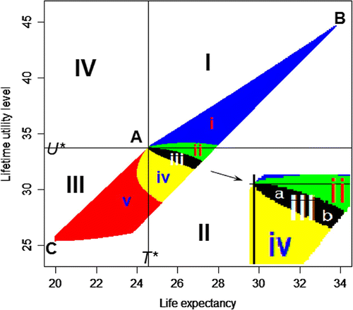
We draw a vertical and horizontal line from the point $\mathtt{A}$ and divide the plain into 4 areas. In area I, the life expectancy is longer and the lifetime utility level is higher compared to the point $\mathtt{A}$. In area II, the life expectancy is longer but the lifetime utility level is lower compared to the point $\mathtt{A}$. In area III, the life expectancy is shorter and the lifetime utility level is lower compared to the point $\mathtt{A}$. In area IV, the life expectancy is shorter and the lifetime utility level is higher compared to the point $\mathtt{A}$. There is no pair in area IV. Furthermore, we have divided the dots into five areas, which are area i, area ii, area iii, area iv and area v, by the government budget constraint as follows:(32) $$\begin{array}{c}\hfill \left\{\begin{array}{cc}\mathrm{area}\mathrm{i},\hfill & \mathrm{if}2sp<(T-s)q\mathrm{extreme}\hfill \\ \mathrm{area}\mathrm{ii},\hfill & \mathrm{if}sp<(T-s)q\le 2sp\mathrm{moderate}\hfill \\ \mathrm{area}\mathrm{iii},\hfill & \mathrm{if}sp=(T-s)q\mathrm{balanced}\hfill \\ \mathrm{area}\mathrm{iv},\hfill & \mathrm{if}\frac{1}{2}sp\le (T-s)q<sp\mathrm{moderate}\hfill \\ \mathrm{area}\mathrm{v},\hfill & \mathrm{if}(T-s)q<\frac{1}{2}sp\mathrm{extreme}\hfill \end{array}\right..\end{array}$$(32)

Figure 2. The areas by the government budget constraint.

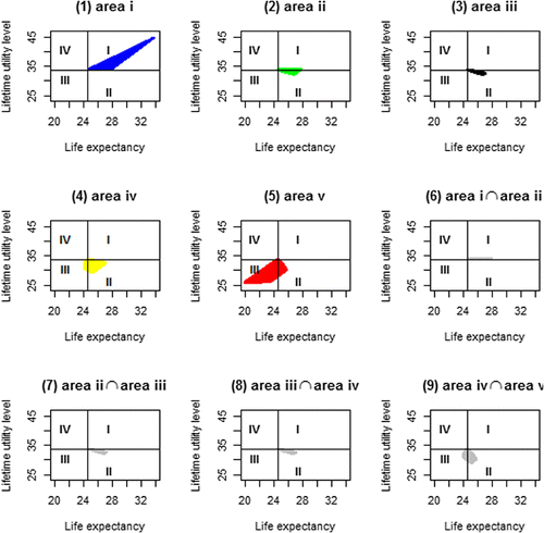
In Figure 2, we depicted each area in detail. Each of the areas was not divided precisely as seen in Figure 1, because there are overlapped areas between the area i and ii, between the area ii and iii, between the area iii and iv, between the area iv and v. We depicted these overlapped areas in (6), (7), (8), and (9) in Figure 2, respectively. When we showed Figure 1, we gave the area ii preference between the area i and ii, which means the area i was plotted first after which the area ii was depicted on the area i. In the overlapped area between the area i and ii, the area ii is on the top because the area i was covered by the area ii. In a similar way, we gave the area iii preference between the area ii and iii; gave the area iii preference between the area iii and iv; and gave the area iv preference between the area iv and v. We prioritized the balanced, the moderate and the extreme to depict the overlapped areas in Figure 1. The existence of the overlapped areas means that even though the government budget is different, the way the pension system is operated can have the same effect on the lifespan and happiness. To put it in another way, even though the government budget is the same, the way the pension system is operated can have a different effect on the lifespan and happiness.

In the area i and ii, the government revenue is less than the government expenditure for the pension. The area i and ii are unfeasible areas if there is no additional financial resources. The government should replenish the underfunded revenue by another way to meet the deficit budget e.g. raising tax or issuance of government bonds or sellout the natural resources, etc. It is an unrealistic assumption. Only few countries, which are rich in natural resources and are carefree about their government resources, for example, oil product countries, may do it. In the area iii, the government executes the balanced budget that can be found in most of the countries in the world.¹⁵ In the area iv and v, the government expenditure for the pension is less than the government revenue. The area iii, iv, and v are feasible areas even if there is no additional financial resources. If pension system has any inefficiency which is liable to happen, the areas, iv and v, are possible.

The pension system can make life expectancy longer or shorter and can make lifetime utility level higher or lower. It is indisputable that if we pay smaller amount of money and get bigger amount of money from our pension, our welfare level will be higher, otherwise, if we pay bigger amount of money, and get smaller amount of money from our pension, our welfare level will be lower. In case of the area I, if we get big amounts of pension in the future, the life expectancy can be extended and the lifetime utility can go up. It is the most preferable, however, in today’s reality, we cannot expect that the amount of the pension will increase due to the problem of financial resources.

In case of the area III, the life expectancy is decreased, moreover, the lifetime utility level can go down. This is the worst scenario. This is the case when he/she is forced to pay his/her pension, he/she chooses a dot in the area III, instead of the point $\mathtt{A}$ which is the best choice for individuals in case without pension system. He/She does not have enough money to invest for his/her health care because most of his/her money is paid for his/her pension. As an extreme example, we can take an individual who can choose a short life to refuse to pay the pension until such period s and to increase his/her consumption in his/her young period.¹⁶

The point $\mathtt{B}$ shows the optimal combination of the life expectancy and the lifetime utility level when we have lowest p, biggest q,  and shortest s. The point $\mathtt{C}$ shows the optimal combination of the life expectancy and the lifetime utility level when we have biggest p, smallest q and longest s. In the point $\mathtt{B}$, the life expectancy is the longest and the lifetime utility level is the highest. On the contrary, in the point $\mathtt{C}$, the life expectancy is the shortest and the lifetime utility level is the lowest. When individuals pay smaller amount of money, and pay for a short period of time, and get bigger amount of money from his/her pension, his/her lifetime utility level will be higher, otherwise, when individuals pay bigger amount of money, and pay for a long period of time, and get smaller amount of money from his/her pension, his/her lifetime utility level will be lower comparing to the case of non-existing the pension system. The result accords with intuition.

In the area II, even though the life expectancy is extended, the lifetime utility level can go down. This is the case when he/she is forced to pay his/her pension, he/she chooses a dot in the area II, instead of the point $\mathtt{A}$ which is the best choice for individuals in case without pension system. Because of that an individual is forced to pay the pension during his/her young period, the pension system leads to less personal consumption in his/her young period. Even though he/she tries to prolong his/her life for a long time to get his/her money back which he/she paid mandatorily, his/her lifetime utility level can go down compared to the case without pension system. Even though rising longevity is incited by the pension system, the years they gain in life expectancy may not be healthy ones, so the increase in life expectancy requires more savings for health-care spending in his/her old age and less consumption through his/her whole life. This is a distortion which can occur due to the pension system.

Let us focus on the area iii which shows the government balanced budget. It is obvious that the pension system only distorts individual’s decision and makes the individual worse off comparing to the point $\mathtt{A}$, because if other things are constant (ceteris paribus), less constrained individual is generally happier than more constrained individual. We have found the fact in the area iii that when the government holds the budget constraint, the lifetime utility level cannot increase. And, we have also found another fact that the life expectancy can prolong even though the lifetime utility level decreases. Individuals know that if they live longer they will get more pension. They are motivated to live longer as it is the only way they could enjoy the pension they have been paying for a long time. This result is consistent with that of Philipson and Becker (1998) even though the model in each research is different. Philipson and Becker (1998) argued that there is a moral hazard effect in annuities that induces excessive longevity. Public annuity programs may distort investments quantity, thereby sacrificing quality, that is, they distort the trade-off toward living longer rather than living well.

In the area ii, when the government expenditures for pension are higher than the government revenues, the life expectancy increases. On the contrary, in the area iv, when the government expenditures for pension are lower than the government revenues, the life expectancy also increases. In the both cases, either the budget surplus or deficit, except the extreme case, the life expectancy prolongs. From these results, we can say that life expectancy can be longer when pension system exists, not only when the government has enough revenue but also when the government hardly has enough revenue.

From Figure 1 which has a positive slope, it can be noticed that there is a positive relationship between life expectancy and lifetime utility level. If we have enough income after retirement, the longer lifespan makes us happier. However, under the government budget constraint, the life expectancy is not always proportional to the lifetime utility level. For example, when we compare the point $\mathtt{a}$ with the point $\mathtt{b}$ in the area iii, even though the life expectancy at the point $\mathtt{b}$ is longer, its lifetime utility level is lower. The extension of lifespan which is caused by the moral hazard effect in public pension without the income support may not always make our happiness higher. The extension of lifespan only chosen by own decision and accompanied by the income support may make our happiness higher. Becker et al. (2005) mentioned that life expectancy gains have been an important component of improvements in welfare, but that may be the case in the situation where their financial problems can be resolved.

3.2. Private savings

3.2.1. Setup

We think another way to finance when an individual lives longer than the planned period T. He/She saves an extra money for the extended period from T to $T+\psi$ in which he/she could be still alive unexpectedly. If the individual is still alive and does not have money after period $T^{\ast }$ which he/she has chosen optimally, he/she will have hard time. So, we assume that first, the individual chooses the $T^{\ast }$ optimally and then he/she maximizes his/her lifetime utility with respect to $T^{\ast }+\psi$ considering the case that he/she will be still alive until $T^{\ast }+\psi$. For example to facilitate the understanding, if that, he/she lives up to 100-year old, is the optimal choice $(T^{\ast })$, the financial plan up to 100-year old will be the best plan. As another choice, he/she considers the uncertainty in his/her life and can plan up to 120-year old $(T^{\ast }+\psi )$ daringly even though the finance of extra 20 years $(\psi )$ may go to waste if he/she dies at 100-year old $(T^{\ast })$. The extra finance is one method to hedge against the uncertainty for himself/herself.

The individual’s utility maximization problem can be written as follows:(33) $$\begin{array}{c}\hfill \underset{c(t)}{max}{\int }_0^{T^{\ast }+\psi }{e}^{-\rho t}lnc(t)dt,\end{array}$$(33)

where $T^{\ast }$ is the optimized T in the benchmark model in the Section 2. In this case, $T^{\ast }$ is given which means that z is given, not a control variable. We can consider two kinds of the maximized utility as follows:(34) $$\begin{array}{cc}\hfill U^I(\psi )& ={\int }_0^{T^{\ast }}{e}^{-\rho t}ln{c}^{\ast }(t)dt+e^{-\rho T^{\ast }}lnx(T^{\ast })\hfill \\ \hfill U^{\mathit{II}}(\psi )& ={\int }_0^{T^{\ast }}{e}^{-\rho t}ln{c}^{\ast }(t)dt,\hfill \end{array}$$(34)

where $c^{\ast }(t)$ is the optimized consumption which is obtained from Equation (33); $x(T^{\ast })$ is the extra finance at $T^{\ast }$ which he/she has saved for the uncertainty; $U^I$ is the utility level in which he/she uses up the extra finance just before he/she dies; and $U^{\mathit{II}}$ is the utility level in which he/she leaves the extra finance when he/she dies, e.g. due to a sudden death.

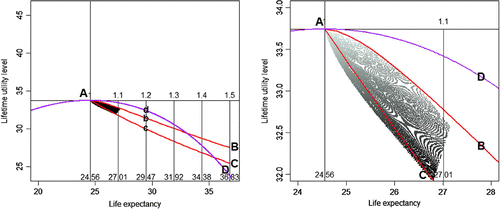
Figure 3. Comparison of public pension and private savings.

3.2.2. Results

We have compared the results of private savings with the results of public pension in the previous section. Figure 3 shows that three lines, which are line $\mathtt{AB}$, line $\mathtt{AC},$ and line $\mathtt{AD}$, are added on Figure 2 (3) area iii which shows the case of balanced budget. The line $\mathtt{AB}$ shows the utility level of the case $U^I$ in which he/she plans the extra finance and uses up the extra finance just before he/she dies. The line $\mathtt{AC}$ shows the utility level of the case $U^{\mathit{II}}$ in which he/she plans the extra finance and leaves the extra finance when he/she dies. For example to facilitate the understanding, the point $\mathtt{b}$ on the line $\mathtt{AB}$ shows the utility level of the following case; he/she decides his/her optimal life expectancy $T^{\ast }$ as 24.56 which means that he/she invests for his/her health 0.456 $(z=\frac{24.56-20}{10})$ and he/she plans up to 29.47 for the uncertainty which is 1.2 times longer than $T^{\ast }$. He/She dies 24.56. He/She uses the extra finance for 4.88 period ($\psi =$29.47$-$24.56) just before he/she dies. The point $\mathtt{c}$ on the line $\mathtt{AC}$ shows the utility level of the following case; he/she decides his/her optimal life expectancy $T^{\ast }$ as 24.56 and he/she plans up to 29.47 for the uncertainty which is 1.2 times longer than $T^{\ast }$. He/She dies 24.56. He/She leaves the extra finance for 4.88 period because of his/her sudden death. The length of $\mathtt{bc}$ is the difference of utility level depending on whether he/she uses the extra finance or not before he/she dies. The line $\mathtt{AB}$ and $\mathtt{AC}$ are downward-sloping which means that the more money he/she saves for the uncertainty, the lower utility level he/she has. The line $\mathtt{AD}$ shows the utility level in relation to the optimal life expectancy when he/she chooses $T^{\ast }+\psi$ as a second best instead of $T^{\ast }$. For example, the point $\mathtt{d}$ on the line $\mathtt{AD}$ shows the utility level of the following case; he/she decides his/her life expectancy as 29.47 which is 1.2 times longer than $T^{\ast }$, which means that he/she invests for his/her health 0.947 $(z=\frac{29.47-20}{10})$. The line $\mathtt{AD}$ is also downward-sloping which means that the further from the optimal life expectancy he/she chooses, the lower utility level he/she has.

The right panel in Figure 3 shows the enlargement of the same area of the left panel in Figure 3. The darker the color gets, the bigger the government budget (sp) is. The upper left part, point $\mathtt{A}$, shows a smaller government budget, inversely, the lower right part shows a bigger government budget. Comparing area iii and line $\mathtt{AC}$, in the case that he/she leaves the extra finance when he/she dies, the utility level when the pension system exists can be greater than the utility level of private saving $U^{\mathit{II}}$. However, comparing area iii and line $\mathtt{AB}$, in the case that he/she uses up the extra finance just before he/she dies, the utility level when the pension system exists can be less than the utility level of private saving $U^I$.

Individuals can hedge against the uncertainty when they finance for extra age for themselves. The public pension cannot make the happiness level higher comparing to the private savings even though the pension system has an insurance effect or a risk-hedging function, because the distortion effect of compulsory pension system is bigger than the value of extra finance. The moral hazard effect in public pension which induces excessive longevity can vanish in the voluntary private savings model.

Bender (2012) analyzed the effect of pension and health on well-being in retirement, in particular, by introducing several different types of pension. Bender (2012) showed that people who have defined contribution (DC) pensions have lower retirement satisfaction than people who have more secured defined benefit (DB) pensions. This result implies that it does not matter whether a pension system exists or not; however, it is vital whether a secure income exists or not. We do not care whether some resources in retirement are pension or own savings as long as the resources are stable. Therefore, the voluntary private savings is better method than the public pension which distorts individual’s decision.

4. Empirical Facts

We have formulated and tested three hypotheses based on the results which we have found in the previous section. We postulate the following hypotheses.

Hypothesis 1 Pension system can make life expectancy longer.

Hypothesis 2 Under the government budget constraint, pension system cannot make the happiness level higher. What is even worse is that pension system can make the happiness level lower.

Hypothesis 3 In case of the extension of lifespan chosen by own decision, the life expectancy is proportional to the happiness. However, in case of the extension of lifespan caused by the moral hazard effect in public pension, the life expectancy itself is not always proportional to the happiness.

4.1. Data

We have used data of happiness, life expectancy, GDP per capita and the existence or non-existence of a pension system to test the three hypotheses. Each of the variables is thought to be the variable that looks at a psychological side, a biological side, an economic side and a social systematic side, respectively. The data used in this research can be easily downloaded on the internet. The happiness index and the life expectancy are available at World Database of Happiness and the GDP per capita is also available at Penn World Table. The data of the existence or non-existence of a pension system are found in Table 1 of Bloom et al. (2007). The World Database of Happiness is a collection of findings on happiness in the sense of the subjective enjoyment of one’s life as-a-whole.¹⁷ World Database of Happiness had released the averages of the happiness index from 2000 to 2009 and the averages of life expectancy from 2000 to 2009 for 10 years. The range of the happiness index is from 0 (unhappiest) to 10 (happiest). The GDP per capita has used the variable “rgdpch" in Penn World Table 7.1. According to the Penn World Table 7.1, the variable “rgdpch" is GDP per capita (chain series) converted using Purchasing Power Parity (PPP), at 2005 constant prices. We have calculated the average of GDP per capita from 2000 to 2009 to meet the happiness index and the life expectancy in World Database of Happiness. The pension data, which are dummy variable for the existence or non-existence of a pension system, show the situation in 2002. The value of dummy variable is one when the country has any pension system and the value of dummy variable is zero when the country does not have any pension system. Regarding pension data, we have used figures under the name “Universal coverage" from the Table 1 of Bloom et al. (2007). According to Bloom et al. (2007), the dummy variable of “Universal coverage" indicates whether the system covers all workers or not.

We have reported the detailed data source in Table 1. World Database of Happiness, Penn World Table 7.1 and the pension data in 2002 of Bloom et al. (2007) listed 149, 190, and 61 countries, respectively. We focus on the 61 countries which have all the three data-sets. Table A1 in the Appendix contains the basic information of the 61 countries. We have to acknowledge that the pension data are rough. There may be both superior and inferior pension systems depending on the countries; however, this data do not include the detail information like the budget surplus or deficit. And also, there are fewer countries without pension system. Only 13 countries out of 61 $(21.3\%)$ do not have their pension system which means 48 countries $(78.7\%)$ have it.¹⁸

Table 1. Data sources

Indicators	Database	Sources
Satisfaction with life (Happiness)	World Database of Happiness	http://worlddatabaseofhappiness.eur.nl/
Life expectancy	World Database of Happiness	http://worlddatabaseofhappiness.eur.nl/
Per capita GDP	Penn World Table	https://pwt.sas.upenn.edu/
Pension	Bloom et al. (2007)	Table 1, Social security systems: retirement and pension provisions, pp. 105–108

Figure 4. Income, happiness, and life expectancy.

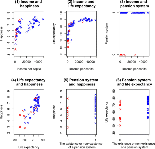
Figure 4 plots the relationship among the four variables which are income per capita, happiness, life expectancy, and the existence or nonexistence of a pension system by combination of these variables. It appears that all of the cases have positive relationships. In Figure 4, os represent the countries that have pension system while on the other side xs represent the countries that do not have any pension system. Figure 4 (1) shows the relationship between income per capita and happiness. In general, people in rich countries are happier than those in poor countries. Happiness across countries shows a moderate positive correlation with income. However, the relationship between income and happiness is concave, not linear relationship. The diminishing marginal utility of income is shown. Figure 4 (2) shows the relationship between income per capita and life expectancy, that is to say Preston curve. People living in rich countries live longer than those living in poor countries. Life expectancy across countries shows a moderate positive correlation with income. However, the relationship between income and life expectancy is also concave, not linear relationship like that shown in Figure 4 (1). Among the poorest countries, increases in average income are strongly associated with increases in life expectancy, but as income per capita rises, the relationship flattens out, and is weaker or even absent among the richest countries. Figure 4 (3) shows the relationship between income per capita and pension system. Poor countries may have pension system or no pension system. However, almost all of rich countries have pension system. Figure 4 (4) shows the relationship between life expectancy and happiness. There is a positive relationship, that is, people who live longer are happier than those who live shorter. Figure 4 (5) shows the relationship between pension system and happiness. The happiness level of countries which have pension system is a little bit higher than the happiness level of countries which do not have pension system. Finally, Figure 4 (6) shows the relationship between pension system and life expectancy. The life expectancy of countries which have pension system is a little bit longer than the life expectancy of countries which do not have pension system. We have reported the coefficients of correlation in Table 2. Even though there is difference in a greater or less degree from 0.390 to 0.788, all of the cases have positive relationships.

Table 2. Coefficients of correlation

Variables	GDP per capita	Happiness	Life expectancy	Pension
GDP per capita	1.000	0.674	0.717	0.436
Happiness	0.674	1.000	0.788	0.390
Life expectancy	0.717	0.788	1.000	0.527
Pension	0.436	0.390	0.527	1.000

4.2. Regression analysis

We can consider a lots of factors that affect happiness. Besides income, those factors include health state, marriage, children, family structure, job, aspiration, personality, age, education, employment, location, culture, ideology, ethnicity, safety/crime, government quality, and stability of the political system. The number of factors is myriad. Frey and Stutzer (2002) and Frey (2008) introduced various independent variables and tested the effect of the variables on satisfaction with life. Bonsanga and Klein (2012) investigated the effect of retirement on life satisfaction with health, income and free time.

To investigate the effect of pension itself on happiness, the effects of other things except for pension which we mentioned above should be removed. However, we only used income per capita to control because it is not easy to get the data from other mentioned factors. We extracted the effect of income on the happiness using non-linear regression, and we computed the purified residual of happiness without the effect of income on happiness. The effect of pension on the purified residual of happiness without the income effect was investigated in linear regression. In the same way, we investigated the effect of pension itself on life expectancy. We extracted the effect of income on the life expectancy using non-linear regression, and we computed the purified residual of life expectancy without the effect of income on life expectancy. The effect of pension on the purified residual of life expectancy without the income effect was investigated in linear regression. We have also analyzed the effect of pension on the residual of happiness and the residual of life expectancy by dividing the countries into two groups, countries with and without pension system.

In order to perform these processes mentioned above, we have considered following regression equations.(35) $$\begin{array}{cc}\hfill L_i& =f(y_i)+{ϵ}_i^L\hfill \\ \hfill H_i& =f(y_i)+{ϵ}_i^H\hfill \\ \hfill {ϵ}_i^L& ={\beta }_0+{\beta }_1{ϵ}_i^H+{\beta }_2{P}_i+{ϵ}_i\hfill \\ \hfill {ϵ}_i^H& ={\beta }_0+{\beta }_1{ϵ}_i^L+{\beta }_2{P}_i+{ϵ}_i\hfill \\ \hfill {ϵ}_i^L& =(1-P_i)({\beta }_0+{\beta }_1{ϵ}_i^H)+P_i({\beta }_2+{\beta }_3{ϵ}_i^H)+{ϵ}_i\hfill \\ \hfill {ϵ}_i^H& =(1-P_i)({\beta }_0+{\beta }_1{ϵ}_i^L)+P_i({\beta }_2+{\beta }_3{ϵ}_i^L)+{ϵ}_i,\hfill \end{array}$$(35)

where the subscripts, ${}_i$s represent country i. And, y, L, H,  and P are the income per capita, the life expectancy, the happiness level and the existence or non-existence of a pension system, respectively. ${ϵ}^H$ is the purified residual of happiness without the effect of income on happiness and ${ϵ}^L$ is the purified residual of life expectancy without the effect of income on life expectancy.

We have considered two regression models on $f(y_i)$ in Equations (35) and (36). As we have seen in the Figure 4, both relationships, between income and happiness and between income and life expectancy, are concave, not linear, so we have introduced two nonlinear models which are power regression model and nonparametric regression model. We have defined the power regression model as follows:(36) $$\begin{array}{c}\hfill f(y_i)={\beta }_0+y_i^{{\beta }_1}.\end{array}$$(36)

We have estimated the variables using nonlinear least-squares regression for Equations (35), (36), (39), and (40), and linear least squares regression for Equations (37) and (38).

4.3. Results

Figure 5. Happiness, life expectancy, and pension system.

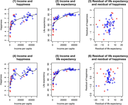
Table 3. Estimation results

	Equation (35)	Equation (36)	Equation (37)	Equation (38)	Equation (39)	Equation (40)
Parameters	Power regression model
${\beta }_0$	48.499	1.644	-2.63	0.169	-2.719	0.189
t value	27.25	5.389	-1.667	0.833	-1.737	0.914
p value	0	0	0.101	0.408	0.088	0.365
${\beta }_1$	0.334	0.169	2.946	0.047	4.634	0.055
t value	45.69	26	3.048	3.048	3.05	2.597
p value	0	0	0.003	0.003	0.003	0.012
${\beta }_2$	-	-	3.342	-0.214	0.696	-0.039
t value	-	-	1.879	-0.934	0.856	-0.375
p value	-	-	0.065	0.354	0.396	0.709
${\beta }_3$	-	-	-	-	1.832	0.038
t value	-	-	-	-	1.485	1.66
p value	-	-	-	-	0.143	0.102
Parameters	Nonparametric regression model
${\beta }_0$	-	-	-2.467	0.238	-2.817	0.248
t value	-	-	-1.591	1.491	-1.791	1.528
p value	-	-	0.117	0.141	0.079	0.132
${\beta }_1$	-	-	2.314	0.024	4.174	0.029
t value	-	-	1.864	1.864	2.097	1.694
p value	-	-	0.067	0.067	0.04	0.096
${\beta }_2$	-	-	3.135	-0.303	0.608	-0.061
t value	-	-	1.788	-1.675	0.761	-0.729
p value	-	-	0.079	0.099	0.45	0.469
${\beta }_3$	-	-	-	-	1.142	0.018
t value	-	-	-	-	0.723	0.865
p value	-	-	-	-	0.473	0.391

Notes: The upper, middle, and lower show the estimated values, t values and p values, respectively. The figures highlighted represent the cases that the result is statistically significant at the 0.10 level.

Figure 5 shows the data, the regression lines, and the residuals. Figure 5 (1), (2), and (3) in the first row show the results of the power regression model and Figure 5 (4), (5), and (6) in the second row show the results of the nonparametric regression model. Table 3 shows the results of both regressions. Let us check the results of the power regression model at first. In Equation (37), ${\beta }_2$ (3.342) is positive and significant which means that the pension can have a positive effect on the longevity. In Equation (38), ${\beta }_2$ (-0.214) is negative but not significant which means that the pension have an insignificant effect on the happiness. In Equation (39), ${\beta }_1$ (4.634) is positive and significant, but ${\beta }_3$ (1.832) is not significant even though positive. In Equation (40), ${\beta }_1$ (0.055) is positive and significant, but ${\beta }_3$ (0.038) is not significant even though positive. These results imply that in case without the pension system, the life expectancy is proportional to the happiness; however, in case with the pension system, the life expectancy is not proportional to the happiness. Next, let us check the results of the nonparametric regression model. In Equation (37), ${\beta }_2$ (3.135) is positive and significant which means that the pension can have a positive effect on the longevity. This result is consistent with the result of the power regression model. In Equation (38), ${\beta }_2$ (-0.303) is negative and significant which means that the pension can have a negative effect on the happiness. This result is different from the result of the power regression model which is not significant even though negative. In Equation (39), ${\beta }_1$ (4.174) is positive and significant, but ${\beta }_3$ (1.142) is not significant even though positive. In Equation (40), ${\beta }_1$ (0.029) is positive and significant, but ${\beta }_3$ (0.018) is not significant even though positive. These results are also consistent with the results of the power regression model.

Table 4. Summary

	the effect of pension on life expectancy	the effect of pension on happiness	the relationship between life expectancy and happiness
			without pension	with pension
Power regression model	Positive	Insignificant	Positive	Insignificant
Nonparametric regression model	Positive	Negative	Positive	Insignificant

We summarized the results of two regressions in Table 4. From both models, we have gotten the consistent result that the effect of pension system on the life expectancy is positive. This means that Hypothesis 1 cannot be rejected. This result is an empirical evidence of the moral hazard effect in public pension mentioned by Philipson and Becker (1998). Next, we have gotten the inconsistent result about the effect of pension system on the happiness.¹⁹ The result of nonparametric regression model is significantly negative, but the result of power regression model is insignificantly negative. The results, insignificant or negative, show there is no significant positive effect. This means that Hypothesis 2 also cannot be rejected. Finally, we have gotten the consistent result about the relationship between life expectancy and happiness level. In case without the pension system, they have a significant positive relationship; however, in case with the pension system, the relationship is insignificant. The extension of lifespan caused by the public pension, not by own decision cannot make happiness level higher. This means that Hypothesis 3 also cannot be rejected. According to the regression results, three hypotheses based on the theoretical model are largely held to be true.

5. Conclusion

This research has analyzed the effect of public pension system on life expectancy and happiness level using the optimal dynamic problem of individuals who live in continuous and finite time and has shown that the results from the model roughly correspond to the characteristics of cross country data.

We have gotten several interesting but radical results from both, the optimization problem and the data. The first result is that the pension system can make life expectancy longer. If the individual does not have to worry about financing future years of living, he/she would want to live longer. This result precisely supports one of the results in Philipson and Becker (1998) that there is a moral hazard effect in public pension that induces excessive longevity. The public pension distorts the trade-off toward living longer rather than living well. This result implies that the pension system can rather raise problems in terms of aging population which affects the country’s productivity and growth rate through the decline in the fraction of working-age population.

The second result is that under government budget constraint, even though the public pension can make the lifespan longer, the public pension cannot make the happiness level higher comparing to the private savings. If there is a pension system, we will try to live longer to get more pension; however, the public pension system which is a compulsory saving can distort individual’s decision and can prevent individual’s utility maximization. Even though the public pension system has an insurance effect and risk-hedging function, unless the prediction of lifespan turns out to be completely wrong, there is a small possibility that the pension system will improve the happiness level because the distortion effect of compulsory pension system is bigger than the value of extra finance which may go to waste in the voluntary private savings. An individual can hedge against the uncertainty if he/she finances for extra age for himself/herself, instead of paying his/her pension. The private savings can increase happiness level comparing to the public pension system.

The third result is that generally, life expectancy itself is proportional to the happiness; however, it is not always true. Prolong lifespan itself is not always making our happiness higher, especially in the case when lifespan is extended by the public pension. The extension of lifespan only chosen by own decision and accompanied by the income support may make our happiness higher.

The anecdote we have mentioned in the head of the introduction is perhaps no accident, but inevitable. It is telling that the jogging was the optimal choice of people who lived during that time to make their lifespan longer. It may be necessary to reconsider the reasons for existence of the compulsory pension system which has been a considerable economic and social burden on young generations.

Many governments are trying to make a new plan not to deplete the national pension fund, e.g. the government’s 100-year safe pension plan in Japan; however, they never seem to succeed, because the pension system has evolved from not only economic circumstance but also demographic, social, cultural and political circumstance, etc. It must be too difficult to develop a perfect plan to solve the pension problem just now. However, the follow things can be considered as some of the partial solutions: (1) shift from pay-as-you-go pension to funded pension; (2) shift from mandatory pension system to private pension system; (3) taxing beneficiaries who are receiving extra benefits from what they have paid; and (4) accurate projection of population, etc.

Acknowledgements

I would like to thank the editor and anonymous referees for their very useful comments and suggestions. I also thank Prof. Dr. Ronnie Sch?b (Freie Universit?t Berlin) for all his help.

Additional information

Funding

The author received no direct funding for this research.

Notes on contributors

Inyong Shin

The author is an economist and statistician. His main research fields are Economic Growth, Computational Economics, Dynamics and Bayesian statistics. His current research area includes developing a public pension system and demography. Public pension systems have been studied in Economics as well as Social Welfare, Sociology, Statistics, etc. In many countries, the national pension fund will start shrinking roughly several decades from now and it’s in danger of disappearing. In the case of Japan, according to a pension specialist, if the Japanese pension systems are operated in that way, National Pension System and Employees’ Pension Insurance System will run out of resources in 2037 and 2033, respectively. Many governments are trying to make a new plan not to deplete the national pension fund, however, they never seem to succeed. The problems of public pension sustainability are great economic and political issues of our time and they need to be solved.

Notes

1 For example, Bloom et al. (2007) and Dushi et al. (2010), Lee et al. (2000) examine the effects of improvements in health or life expectancy on social security system and saving rate. Weil (2007), Acemoglu and Johnson (2007), Zhang et al. (2001), and so on, analyze the effects of improvements in health or life expectancy on economic growth. Zhang et al. (2003) shows that rising longevity encourages both savings and earlier retirement. Zhang and Zhang (2005) show that rising longevity raises saving, schooling time and economic growth at a diminishing rate. Gorski et al. (2007) studies the effects of a pension reform on the educational level of the economy. Pecchenino and Utendorf (1999), de la Croix and Licandro (1999), Cipriani (2000), Boucekkine et al. (2002, 2003), Pecchenino and Pollard (1997, 2002), and so on, analyze the effect of longer lifespan on economic growth through the level of schooling and human capital accumulation. Lorentzen, McMillan and Wacziarg (2008) and Chakraborty et al. (2010), and so on, analyze the effect of mortality and disease on economic growth and growth trap. Lorentzen et al. (2008) mentions that higher adult mortality has bad influences on economic growth and could be the source of a poverty trap through increased levels of risky behavior, higher fertility, and lower investment in physical and human capital. Zhang and Zhang (2004) investigates how social security interacts with growth and growth determinants and shows that social security may indeed be conducive to growth.

2 For example, there are many people who still smoke, even though they know all of the health risks and there are so many warnings and pictures showing the consequences on the cigarette packets. We can interpret their behavior by saying that they prefer some present pleasure from smoking, even if smoking plays havoc with their health. It can be an example of the first case, that is, they choose to live a short and intensely happy life.

3 For example, eating good food, taking some nutritional supplements, getting in shape by going to the gym, investing in the development of medical technology, and so on. The longevity will arise due to the implementation of the previously mentioned examples of the health investments. In reality, it is well known that coronary heart disease (CHD) mortality is highly influenced by the major risk factors, e.g. serum cholesterol, systolic blood pressure, diabetes, smoking habits, high alcohol consumption, lack of exercise and stress, etc. Lifestyle changes through individual’s efforts (e.g. healthier diet, physical exercise, cessation of smoking, drinking, etc.) and medications have been shown to be effective in reducing coronary disease. If we can eliminate the risk factors, the life expectancy will undoubtedly grow.

4 According to Kimball and Willis (2006), Bentham (1781) first definition of “utility" made the equation of utility and happiness explicit. Kimball and Willis (2006) mentioned that in the existing literature attempting to link utility and happiness, the dominant explicit or implicit hypothesis is that current felt happiness is equal to flow utility. Kahneman (1999), Gruber and Mullainathan (2002), Frey and Stutzer (2004), and Layard (2005) are some of the most explicit in equating happiness and flow utility. Bonsanga and Klein (2012) use interchangeably, the expressions subjective well-being, satisfaction with life, general satisfaction, life satisfaction, and satisfaction with life in general.

5 We can divide consumption c into two categories which are the general consumption $c^G$ and the consumption for health improvement $c^H$. It is unclear whether the direct effect of the latter $c^H$ on the utility of individual is positive or negative or neutral. For examples, there might be a person who takes wheatgrass powder for his/her health maintenance even though it is unpalatable, while on the other side, there might be a person who takes it with the thinking that it is delicious. Also, there might be a person who commutes to the gym for his/her health maintenance though it is painful, while on the other side, there might be a person who goes happily to the gym. Nutritional supplements are beneficial for health but are not delicious or tasteless. Therefore, we can assume that the consumption for health improvement $c^H$ is neutral to the individual’s utility and only the general consumption $c^G$ affects the individual’s utility. This means $\frac{\partial v(c^G,c^H)}{\partial c^G}>0$ and $\frac{\partial v(c^G,c^H)}{\partial c^H}=0$, so $v(c^G,c^H)=u(c^G)$.

6 Dalgaard and Strulik (2014) introduce a wage income as a constant value during life. In Japan, in case of people who are over pension eligibility age and continue to work and get more than 280,000 Japanese yen monthly, their pension can be reduced. If the wage income is introduced in our model, we should also consider the optimal retirement age to get money from our pension. This makes our problem complicated. This research focuses on the optimal longevity. The study on optimal retirement age may be a subject of our future studies.

7 If $r=\rho$, there is no transitional path, because the jump from the initial state up to the terminal state occurs. If $r<\rho$, there is an overshooting, the amount of his/her asset accumulation turns back to the terminal state and has a negative growth rate. We do not consider the negative growth in this research.

8 Ehrlich and Chuma (1990) and Dalgaard and Strulik (2014) derived time path for health investment/cost. The aim of this research is to calculate the longevity T and the lifetime utility level U, not to calculate how to change the health investments over time. Even though we deal with z as a state variable, not constant, the results won’t change drastically.

9 When we use the numerical method to solve the T, depending on computer software, Equation (19), which is the reduced form of maximized lifetime utility function with T, is not necessary, but with the reduced form, it is easier to understand the marginal effects of parameters on the maximized lifespan utility comparing to a structural form.

10 The figure does not mean the number of years. The absolute value does not have any meanings until it is compared as the concept of the ordinal utility.

11 We can see that Equation (18) is concave against T visually in Figure 3.

12 There are many different ways to express the lifetime uncertainty problem, for example, we can model the uncertainty problem as follows, $maxE(U)={\int }_{-\infty }^{\infty }U(c|ϵ)f(ϵ)dϵ$, where $f(ϵ)$ means probability density function. However, this assumption makes the uncertainty problem very simple. We do not need to specify about the distribution of random variable $ϵ$, etc.

13 As the population ages and fewer babies are born, pension system might cause inequality problem between young generation and old generation.

14 We only consider the unchanged period in population structure, which means the population structure is in the steady state, not in transitional path.

15 To be precise, $sp\simeq (T-s)q$. We use the grid search so $\left|\frac{sp-(T-s)q}{\mathit{sp}}\right|\le$ 0.01 is regarded as equal.

16 There was an accident reported in South Korea in 2005, where a person, who was against the compulsory pension system and who was in arrears with his pension, took away his life. Also, on 30 June 2015, there was an incident where a passenger committed suicide by setting himself on fire on a shinkansen bullet train in Japan. He had repeatedly complained that his pension was too low, he only received a pension of 240,000 Japanese yen every two months, despite having made payments for 35 years. For more details, check Japan Times on July 2nd 2015. http://www.japantimes.co.jp/news/2015/07/02/national/crime-legal/shinkansen-suicide-victim-tried-buy-gas-near-home-reportedly-short-distance-ticket/

17 See Veenhoven, R., World Database of Happiness, Erasmus University Rotterdam, The Netherlands. Assessed on 1st/Jan/2016 at: http://worlddatabaseofhappiness.eur.nl for details.

18 Collecting the data over time can helpful to overcome the problem of the rough data. This time it is not easy to get the data, so we had no choice but to use the rough data.

19 To be more precise, the budget constraint data should have been used that is which countries are in balanced budget, surplus or deficit. However, it was not easy to get the information for this research.

Appendix 1

Appendix

Derivation of Equation (11)

Let us put $B=-C_1^{-1}$. Multiplying both sides of Equation (10) by $e^{-rt}$ and integrating to time t, we get the following(37) $$\begin{array}{cc}\hfill (\dot{x}-rx+z)e^{-rt}& =B{e}^{-\rho t}\hfill \\ \hfill x{e}^{-rt}-\frac{z}{r}{e}^{-rt}+D_1& =-B\frac{e^{-\rho t}}{\rho }+D_2,\hfill \\ \hfill \end{array}$$(37)

where $D_1$ and $D_2$ are constants of integration. Equation (37) can be arranged as follows:(38) $$\begin{array}{cc}\hfill x{e}^{-rt}-\frac{z}{r}{e}^{-rt}& =-B\frac{e^{-\rho t}}{\rho }+B\frac{1}{\rho }+C_2\hfill \\ \hfill (x-\frac{z}{r})e^{-rt}& =-B(\frac{e^{-\rho t}-1}{\rho })+C_2\hfill \end{array}$$(38)

where $C_2=D_2-D_1-B\frac{1}{\rho }$. Multiplying both sides of Equation (43) by $e^{-rt}$ and substituting $B=-C_1^{-1}$ into Equation (38), Equation (38) can be arranged as Equation (11).

Derivation of Equation (17)

Let us put $A=ln(\rho \frac{x_0-(1-e^{-rT})\frac{z}{r}}{1-e^{-\rho T}})$.(39) $$\begin{array}{cc}& {\int }_0^T{e}^{-\rho t}ln(\rho \frac{x_0-(1-e^{-rT})\frac{z}{r}}{1-e^{-\rho T}}{e}^{(r-\rho )t})dt\hfill \\ \hfill =& {\int }_0^T[A{e}^{-\rho t}+(r-\rho )t{e}^{-\rho t}]dt=A{\int }_0^T{e}^{-\rho t}dt+(r-\rho ){\int }_0^{T}t{e}^{-\rho t}dt\hfill \\ \hfill =& A[-\frac{e^{-\rho t}}{\rho }{]}_0^T-(r-\rho )[\frac{(\rho t+1)e^{-\rho t}}{{\rho }^2}{]}_0^T=-A(\frac{e^{-\rho T}-1}{\rho })-(r-\rho )(\frac{(\rho T+1)e^{-\rho T}-1}{{\rho }^2})\hfill \end{array}$$(39)

Substituting $A=ln(\rho \frac{x_0-(1-e^{-rT})\frac{z}{r}}{1-e^{-\rho T}})$ into Equation (39), Equation (39) can be arranged as Equation (17).

Table A1. Data

	Country	Pension	Happiness	Life expectancy	GDP per capita
1	Argentina	1	7.3	74.8	9687
2	Australia	1	7.7	80.9	37863
3	Austria	1	7.6	79.4	36075
4	Belgium	1	7.3	78.8	33656
5	Bolivia	1	6.3	64.7	3331
6	Brazil	1	7.5	71.7	7297
7	Burkina Faso	0	4.4	51.4	831
8	Canada	1	7.8	80.3	35836
9	Chile	1	6.7	78.3	10783
10	Colombia	0	7.7	72.3	6514
11	Denmark	1	8.3	77.9	34283
12	Dominican Republic	1	7.5	71.5	8215
13	Ecuador	1	6.4	74.7	5374
14	Egypt	1	5.7	70.7	4059
15	Finland	1	7.9	78.9	31840
16	France	1	6.6	80.2	30952
17	Germany	1	7.1	79.1	32214
18	Ghana	1	5.2	59.1	1659
19	Greece	1	6.4	78.9	24764
20	Hong Kong	1	6.6	81.9	32048
21	India	0	5.5	63.7	2466
22	Indonesia	0	6.3	69.7	3192
23	Ireland	1	7.6	78.4	38301
24	Israel	1	7.0	80.3	23533
25	Italy	1	6.7	80.3	29384
26	Jamaica	1	6.7	72.2	8930
27	Japan	1	6.5	82.3	30858
28	Kenya	1	3.7	52.1	1141
29	Korea, South	1	6.0	77.9	22254
30	Madagascar	1	3.7	58.4	725
31	Malaysia	1	6.5	73.7	10366
32	Mali	1	4.7	53.1	862
33	Mexico	1	7.9	75.6	11611
34	Morocco	0	5.4	70.4	3006
35	Netherlands	1	7.6	79.2	36687
36	New Zealand	1	7.5	79.8	26436
37	Nigeria	0	5.7	46.5	1527
38	Norway	1	7.9	79.8	48534
39	Panama	0	7.8	75.1	8095
40	Peru	1	6.2	70.7	5642
41	Philippines	1	5.9	71.0	2753
42	Portugal	1	5.7	77.7	20032
43	Senegal	1	4.5	62.3	1374
44	Singapore	1	6.9	79.4	42103
45	South Africa	1	5.8	50.8	6697
46	Spain	1	7.2	80.5	27852
47	Sri Lanka	1	5.1	71.6	3186
48	Sweden	1	7.8	80.5	33235
49	Switzerland	1	8.0	81.3	37295
50	Taiwan	0	6.2	76.4	26107
51	Tanzania	0	2.8	51.0	913
52	Tunisia	1	5.9	73.5	5692
53	Turkey	1	5.6	71.4	9084
54	Uganda	0	4.8	49.7	959
55	United Kingdom	1	7.2	79.0	33166
56	United States	1	7.4	77.9	41327
57	Uruguay	1	6.7	75.9	8927
58	Venezuela	1	7.5	73.2	8876
59	Viet Nam	0	6.1	73.7	2014
60	Zambia	0	5.0	40.5	1156
61	Zimbabwe	0	3.0	40.9	337
	Average	0.79	6.4	71.2	16622
	Min	0	2.8	40.5	337
	Max	1	8.3	82.3	48534

References

- Acemoglu, D., & Johnson, S. (2007). Disease and development: The effect of life expectancy on economic growth. Journal of Political Economy, 115(6), 925–985.
- Becker, G. S., Philipson, T. J., & Soares, R. R. (2005). The quantity and quality of life and the evolution of world inequality. American Econonmic Review, 95(1), 277–291.
- Bender, K. A. (2012). An analysis of well-being in retirement: The role of pensions, health, and ‘voluntariness’ of retirement. Journal of Socio-Economics, 41(4), 424–433.
- Bentham, J. (1781). An introduction to the principles of morals and legislation. Retrieved from http://www.utilitarianism.com/jeremy-bentham/index.html
- Bloom, D. E., Canning, D., Mansfield, R. K., & Moore, M. (2007). Demographic change, social security systems, and savings. Journal of Monetary Economics, 54(1), 92–114.
- Bohn, H. (2009). Intergenerational risk sharing and fiscal policy. Journal of Monetary Economics, 56(6), 805–816.
- Bonsanga, E., & Klein, T. J. (2012). Retirement and subjective well-being. Journal of Economic Behavior & Organization, 83(3), 311–329.
- Boucekkine, R., de la Croix, D., & Licandro, O. (2002). Vintage human capital, demographic trends, and endogenous growth. Journal of Economic Theory, 104(2), 340–375.
- Boucekkine, R., de la Croix, D., & Licandro, O. (2003). Early mortality decline at the dawn of modern growth. Scandinavian Journal of Economics, 105(3), 401–418.
- Chakraborty, S. (2004). Endogenous lifetime and economic growth. Journal of Economic Theory, 116(1), 119–137.
- Chakraborty, S., Papageorgiou, C., & Pérez-Sebastián, F. (2010). Diseases, infection dynamics and development. Journal of Monetary Economics, 57(7), 859–872.
- Cipriani, G. P. (2000). Growth with unintended bequests. Economics Letters, 68(1), 51–53.
- Cutler, D. M., & Gruber, J. (1996). Does public insurance crowd out private insurance? Quarterly Journal of Economics, 111(2), 391–430.
- de la Croix, D., & Licandro, O. (1999). Life expectancy and endogenous growth. Economics Letters, 65(2), 255–263.
- Dalgaard, C.-J., & Strulik, H. (2014). Optimal aging and death: understanding the Preston Curve. Journal of the European Economic Association, 12(3), 672–701.
- Deaton, A. (2003). Health, inequality, and economic development. Journal of Economic Literature, 41(1), 113–158.
- Dushi, I., Friedberg, L., & Webb, T. (2010). The impact of aggregate mortality risk on defined benefit pension plans. Journal of Pension Economics and Finance, 9(4), 481–503.
- Ehrlich, I., & Chuma, H. (1990). A model of the demand for longevity and the value of the life extension. Journal of Political Economy, 98(4), 761–782.
- Feldstein, M. S., & Liebman, J. B. (2002). The distributional aspects of social security and social security reform. NBER Chapters (pp. 263–326). National Bureau of Economic Research.
- Frey, B. S., & Stutzer, A. (2002). Happiness and economics: How the economy and institutions affect human well-being. Princeton: Princeton University Press.
- Frey, B. S., & Stutzer, A. (2004). Economic consequences of mispredicting utility, Institute for Empirical Research in Economics (Working Paper No.218),
- Frey, B. S. (2008). Happiness: A revolution in economics. Cambridge, MA: MIT Press.
- Gorski, M., Krieger, T., & Lange, T. (2007). Pensions, education and life expectancy (Working Papers Series No.2007-02). Paderborn: University of Paderborn, Center for International Economics.
- Grossman, M. (1972). On the concept of health capital and the demand for health. Journal of Political Economy, 80(2), 223–255.
- Gruber, J., & Mullainathan, S. (2002). Do cigarette taxes make smokers happier? (NBER Working Paper No.8872),
- Kahneman, D. (1999). Objective happiness, Chapter 1 in Daniel Kahneman. In E. Diener & N. Schwarz (Eds.), Well-being: The foundations of hedonic psychology. New York: Russell Sage Foundation.
- Kimball, M., & Willis, R. (2006). Utility and happiness., Retrieved from http://www-personal.umich.edu/mkimball/pdf/uhap-3march6.pdf
- Krueger, D., & Kubler, F. (2002). Intergenerational risk sharing via social security when markets are incomplete. American Economic Review, 92(2), 407–410.
- Layard, R. (2005). Happiness. London, UK: Penguin Press.
- Lee, R., Mason, A., & Miller, T. (2000). Life cycle savings and demographic transition: the case of Taiwan. Population and Development Review, 26, 194–219.
- Lorentzen, P., McMillan, J., & Wacziarg, R. (2008). Death and development. Journal of Economic Growth, 13(2), 81–124.
- Momota, A., Tabata, K., & Futagami, K. (2005). Infectious disease and preventive behavior in an overlapping generations model. Journal of Economic Dynamics and Control, 29(10), 1673–1700.
- Pecchenino, R. A., & Pollard, P. S. (1997). The effects of annuities, bequests, and aging in an overlapping generations model of endogenous growth. Economic Journal, 107, 26–46.
- Pecchenino, R. A., & Pollard, P. S. (2002). Dependent children and aged parents: Funding education and social security in an aging economy. Journal of Macroeconomics, 24(2), 145–169.
- Pecchenino, R. A., & Utendorf, K. R. (1999). Social security, social welfare and the aging population. Journal of Population Economics, 12(4), 607–623.
- Pestieau, P., & Ponthiere, G. (2012). The public economics of increasing longevity. Review of Public Economics, 200, 41–74.
- Philipson, T. J., & Becker, G. S. (1998). Old-age longevity and mortality-contingent claims. Journal of Political Economy, 106(3), 551–573.
- Ponthiere, G. (2009). Rectangularization and the rise in limit-longevity in a simple overlapping generations model. The Manchester School, 77(1), 17–46.
- Sánchez-Marcos, V., & Sánchez-Martin, A. R. (2006). Can social security be welfare improving when there is demographic uncertainty? Journal of Economic Dynamics and Control, 30(9–10), 1615–1646.
- Shiller, R. (1999). Social security and institutions for intergenerational, intragenerational and international risk sharing. Carnegie-Rochester Conference Series on Public Policy, 50(1), 165–204.
- Weil, D. N. (2007). Accounting for the effect of health on economic growth. Quarterly Journal of Economics, 122(3), 1265–1306.
- Zhang, J., & Zhang, J. (2004). How does social security affect economic growth? Evidence from cross-country data. Journal of Population Economics, 17(3), 473–500.
- Zhang, J., & Zhang, J. (2005). The effect of life expectancy on fertility, saving, schooling and economic growth: Theory and evidence. Scandinavian Journal of Economics, 107(1), 45–66.
- Zhang, J., Zhang, J., & Lee, R. (2001). Mortality decline and long-run economic growth. Journal of Public Economics, 80(3), 485–507.
- Zhang, J., Zhang, J., & Lee, R. (2003). Rising longevity, education, savings, and growth. Journal of Development Economics, 70(1), 83–101.