Expected lifetime range ratio to find mean reversion: Evidence from Indian stock market

Abstract

We use the expected lifetime range (ELR) ratio based on the extreme values of asset prices to detect the presence of mean reversion in stock returns. We find that the actual cross-sectional average of the ELR ratio is significantly less than its bootstrap means, thereby indicating a considerable amount of mean reversion. We argue that ELR ratio is more conclusive in detecting mean reversion when compared to the traditional Lo and MacKinlay variance ratio variance ratio. On the empirical side, we find that mean reversion is a robust feature among the constituents of India’s BSE SENSEX stock index.

Keywords:

• mean reversion
• extreme value estimators
• expected lifetime range ratio
• Lo and MacKinlay variance ratio
• random walk

JEL classification:

• C12
• C15
• C58
• G10

PUBLIC INTEREST STATEMENT

Suppose, if stock prices move randomly over a period of time, then it becomes impossible for an informed or uninformed investor to predict the future price of an asset. However, if the stock prices follow mean reversion, then it becomes at least partially possible for an investor to predict the future price of an asset based on the movement of the past prices over a period of time. Hence, it becomes essential for any investor to understand the movement of the stock prices over a period of time. That is, an investor can make better investment in asset markets if he knows whether stock prices are moving randomly or having mean reverting behavior. In this research article, we come up with a model which captures the mean reverting behavior in a stock market in a much better way when compared to the existing model in the literature.

1. Introduction

It is well established in financial time series literature, that if stock prices follow the random walk behavior, one cannot predict future stock returns based on the history of past returns. On the other hand, if the stock prices follow mean reverting behavior, it is possible to at least partially predict future returns based on the past returns as any shock to stock prices has a temporary component and there exists a tendency for the price series to return to its trend or path over time. Hence, it becomes important to understand the behavior of the stock price movements, i.e., whether the stock prices follow random walk or mean reversion. In this article, we contribute to the literature using the expected lifetime range (ELR) ratio to detect the presence of mean reversion in stock returns using the extreme values of asset prices unlike the traditional variance ratio tests proposed by Lo and MacKinlay (1988) which is based on closed prices alone.

Mean reversion in financial markets is credited to overreaction to short-term events which are often not realized in the long-term. In the literature, one of the earliest observations about overreaction in markets has been made by Keynes (1936): “The day-to-day variations in the profits of existing investments, which are obviously of a short-lived and ephemeral nature, have an altogether excessive, and even an absurd, influence on the market.” Mean reversal or momentum in stock prices is far away from the efficient market hypothesis, or equivalently that stock prices do not follow random walks.

Shiller (1981) concludes that dividends do not rationally explain stock price movements, because there is excess volatility due to overreaction. The experimental evidence of Tversky and Kahneman (1981) suggests that subjects tend to overreact to new information in probabilistic judgments. De Bondt and Thaler (1985) tested the overreaction theory for monthly return data for New York Stock Exchange (NYSE) common stocks for the period between January 1926 and December 1982 and found that the overreaction effect is asymmetric: it is much larger for losers than for winners. That is, in revising their beliefs, individuals overweight recent information and underweight prior data.

It was reported in the survey article (Fama 1970) that most of the studies were unable to reject the efficient market hypothesis for common stocks. Summers (1986) examines the power of the statistical tests commonly used to evaluate the efficiency of the speculative markets. The presence of long memory or mean reversion in stock markets supports the notion of market inefficiency. Although unit root tests¹ are widely used to test the random walk hypothesis² in the literature, they suffer from the drawback of having low power against the alternative of mean reversion in small samples (DeJong, Nankervis, Savin, and Whiteman 1992). Therefore, even the rejection of random walk hypothesis does not let us interpret that there exists mean reversion.

The other alternative test in the study of the random walk hypothesis is the variance ratio (VR) test. Poterba and Summers (1988) used VR test to check for mean reverting behavior in stock returns. The random walk hypothesis is strongly rejected for equal-weighted and value-weighted portfolios based on stocks from NYSE and AMEX for the period 1962–1985 using weekly returns based on the simple specification test proposed by Lo and MacKinlay (1988). Furthermore, since the variance ratio for different holding periods is more than unity, it cannot be explained by the mean reversion property of asset prices.

Lo and MacKinlay (1988) test is based on the assumption that returns are at least identically distributed, if not normally distributed and the variance of the random walk increments in finite sample is linear in sampling interval. The limitation of LM test is that they are asymptotic tests. Even though the VR test is quite powerful against homoscedastic or heteroscedastic i.i.d. null hypothesis as per Smith and Ryoo (2003), the sampling distribution of the VR statistic can be far from normal in finite samples, showing severe bias and skewness. In relatively small samples, VR tests can suffer from serious test-size distortions or low power as per Lo and MacKinlay (1989) using Monte Carlo methods. Other studies in the existing literature on mean reversion in stock prices include the panel data tests (Chaudhuri and Wu, 2004; Narayan and Smyth, 2005; Narayan and Smyth, 2007; Choi and Chue, 2007), bootstrap tests (Caporale and Gil-Alana, 2002; Mukherji 2011), and tests for nonlinear behavior in mean reversion process (Lim and Liew, 2007; Turan et al. 2008).

The recent growth in equity markets and in emerging markets has created much interest in both practitioners and academics. Emerging markets have seen a huge inflow of capital that increases the cross-border investment. Some of the articles on emerging markets in the literature include the works of Harvey (1995), Madhusoodanan (1998), Malliaropulos and Priestley (1999), Chaudhuri and Wu (2004), Lock (2007), Al-Khazali, Ding, and Pyun (2007), Wang, Zhang, and Zhang (2015), and Neaime.S (2015). The recent work by Maheswaran, Balasubramanian, and Yoonus (2011) has found significant evidence of excess volatility in stock prices in India by way of excessive path dependence.

In this article, we make use of the ELR ratio, based on high and low prices, to test for the presence of mean reversion in the emerging Indian stock market³. What we find is that the cross-sectional (CS) average of the actual ELR ratio is significantly less than its bootstrap mean, indicating there is a considerable amount of mean reversion. Interestingly enough, we also find that the CS average of the traditional LM statistic proposed by Lo and MacKinlay (1988), based on closing prices alone, is equal to its bootstrap mean, which would ordinarily be taken to imply that there is no mean reversion. This is so because the LM statistic has less power to reject the null hypothesis of random walk and fails to find the evidence of mean reversion. We document that ELR ratio is superior to LM statistic in detecting the evidence of mean reversion in the stock markets.

The rest of the article is organized as follows. In Section 2, we explain the ELR ratio and the Lo and MacKinlay (LM) variance ratio statistic in the MA (1) specification model. In Section 3, we perform Monte Carlo simulation experiments for different number of steps and MA (1) parameter $\theta$ to find the connection of ELR and LM statistic to mean reversion. In Section 4, we show the empirical evidence in the data on the presence of mean reversion in the Indian stock market. In Section 5, we undertake a check on the robustness of our findings by analyzing sub-samples periods from before and after the global financial crisis of 2008. In Section 6, we conclude the article with a summary of our main findings.

2. Methodology

Let us define the stock price for n steps as

$S_n=x_1+x_2+x_3+\dots +x_n$

where $S_0=0$ and then $x_i$ follow an MA (1) model given by:

(1) $x_i={ϵ}_i+\theta {ϵ}_{i-1},i\ge 1,\left|\theta \right|\le 1$(1)

where ${ϵ}_i$ are independently and identically distributed as N (0,1). It is easy to see from Equation (1) that

$\mathbb{E}(x_i)=0,\mathrm{\&}$

$Var(x_i)=1+{\theta }^2$

$Cov(x_i,x_{i-1})=\theta$

Therefore, the first order autocorrelation is given by

(2) $\rho (1)=\frac{\theta }{1+{\theta }^2}$(2)

Let the normalized series of partial sums for $0\le n\le N$ be given by

${\tilde{S}}_n=\frac{1}{\sqrt{N}}{S}_n$

By making use of the Functional Central Limit Theorem (FCLT), we can show that, as $N$ gets large, the sequence $\{{\tilde{S}}_n:0\le n\le N\}$ converges to the Brownian Motion with zero mean and variance equal to ${\sigma }^2$, where ${\sigma }^2=(1+\theta {)}^2$ and $\theta$ is the MA (1) parameter.

Now let us make use of the results of Cochrane (1988) and Lo and MacKinlay (1988) to express the LM variance ratio in terms of autocorrelation coefficients as

(3) $\begin{array}{cc}LM=\frac{Var({\tilde{S}}_N)}{Var(x_1)}& =1+2\sum _{j=1}^{N-1}(1-\frac{j}{N})\rho (j)\\ \hspace{0.17em}& =1+2(1-\frac{1}{N})\rho (1)\\ \hspace{0.17em}& =\frac{{(1+\theta )}^2}{(1+{\theta }^2)}\end{array}$(3)

where $\rho (j)=0,\mathrm{\forall }j\ge 2$

According to the LM variance ratio statistic, the null hypothesis is that the variance ratio = 1, and the alternate hypothesis is that variance ratio is not equal to 1.

If the null of random walk is rejected and the variance ratio > 1, then positive first order autocorrelations do exist in the return series, and hence, variances of returns grow faster than linearly (mean aversion).

If the null is rejected and variance ratio is < 1, then negative first order correlation is detected in return series, and hence, variance of returns grow slowly than linearly (mean reversion).

Now let us define the ELR ratio in terms of the first order autocorrelation coefficients.

Let ${\tilde{M}}_n$ be the maximum and ${\tilde{m}}_n$ be the minimum of ${\tilde{S}}_n$, the normalized series of partial sums, for $0\le n\le N$. Based on the FCLT, we can show that

$\underset{N\to \mathrm{\infty }}{lim}\mathbb{E}({\tilde{M}}_N)=2\varphi (0)\sigma$

where $\varphi (z)$ is the standard normal density function. Using the symmetry of $S_n$, it follows that

$\mathbb{E}({\tilde{M}}_N)=\mathbb{E}(-{\tilde{m}}_N)$

Therefore, the expectation of the normalized N-step range is given by:

(4) $\underset{N\to \mathrm{\infty }}{lim}\mathbb{E}({\tilde{R}}_N)=4\varphi (0)\sigma$(4)

To find the ELR ratio, we need to consider the base case when N = 1.

If $x_1>0$, then $M_1=x_1,m_1=0$ and so, $R_1=x_1$. Similarly

If $x_1<0$, then $M_1=0,m_1=x_1$ and so, $R_1=-x_1$.

Thus we have,

$\mathbb{E}(R_1)=\mathbb{E}(\left|x_1\right|)$

Also from Equation (1), we know that $x_1\sim N(0,1+{\theta }^2).$ Therefore, we can write

$\mathbb{E}(R_1)=\sqrt{1+{\theta }^2}\left\{\frac{\mathbb{E}(\left|x_1\right|)}{\sqrt{1+{\theta }^2}}\right\}$

where $\left\{\frac{\mathbb{E}(\left|x_1\right|)}{\sqrt{1+{\theta }^2}}\right\}\sim N(0,1).$

Using the properties of standard normal density, it can be shown that if $Z\sim N(0,1)$ then $\mathbb{E}(\left|Z\right|)=2\varphi (0)$. Therefore, we have,

(5) $\mathbb{E}({\tilde{R}}_1)=2\varphi (0)\sqrt{1+{\theta }^2}$(5)

By combining Equations (4) and (5), we get that

(6) $\begin{array}{cc}\mathrm{E}\mathrm{L}\mathrm{R}\mathrm{R}\mathrm{a}\mathrm{t}\mathrm{i}\mathrm{o}& =\frac{\underset{N\to \mathrm{\infty }}{lim}\mathbb{E}({\tilde{R}}_N)}{\mathbb{E}({\tilde{R}}_1)}\\ \hspace{0.17em}& =\frac{2(1+\theta )}{\sqrt{1+{\theta }^2}}\end{array}$(6)

Naturally, we are interested in estimating the MA (1) parameter $\theta$ based on data. Using the first order autocorrelation of the close-to-close return and Equation (14), we get that

$\rho =\frac{\theta }{1+{\theta }^2}where\left|\theta \right|\le 1and\left|\rho \right|\le 0.5$

which implies that

$\theta =\frac{1}{2\rho }\pm \sqrt{{\frac{1}{2\rho }}^2-1}$

Since it must be that $\left|\theta \right|\le 1$, the only admissible solution is given by:

(7) $\theta =x-sign(\rho )\sqrt{x^2-1}$(7)

where $x=\frac{1}{2\rho }$.

We can show that ELR ratio will be less than its bootmean⁴ (mean reversion) if and only if the LM statistic is less than its bootmean (mean reversion) and vice versa, in case of the fixed parameter $\theta$ in the MA (1) model. However, when we consider the stochastic parameter $\tilde{\theta }$ in the MA (1) model, we can show that ELR ratio will be less than its bootmean (mean reversion) even when the LM statistic is not less than its bootmean (no mean reversion).

Now let us show that the ELR ratio will always be increasing with respect to $k$-day when daily returns are independent over time, unlike the LM statistic which stays flat at unity for all $k$-day. In order to do so, we work with the Gaussian random walk with $N$ steps, with drift $\mu$ and unit variance. We make use of Spitzer’s Identity given in Spitzer (1956) to compute the level of ELR for various $N$ and then convert it to the ELR ratio defined with respect to initial $N$=1.

From Table 1, we observe that ELR ratio⁵ for $k$-day = 1 is equal to 1 for $\mu =0,\pm 1,\pm 2$ . Also, we observe that the ELR ratio increases as $k$-day increases from $k$-day = 1 to k-day = 20. We also find that the rate at which the ELR ratio increases with respect to the $k$-day decreases as the $\left|\mu \right|$ increases. That is to say, the value of ELR ratio from $k$-day = 1 to $k$-day = 20 increases from 1 to 1.70 when $\mu =0,1$ to 1.39 when $\left|\mu \right|=1$ and from 1 to 1.13 when $\left|\mu \right|=2$.

Table 1. ELR ratio for $\mu =0,\left|\mu \right|=1,\left|\mu \right|=2$ for different $k$-days

ELR ratio	k-day	1	2	3	4	5	6	7	8	9	10	11	12	13	14	15	16	17	18	19	20
	$\left|\mu \right|=\mathbf{2}$	1.00	1.02	1.04	1.05	1.06	1.07	1.08	1.09	1.09	1.10	1.10	1.11	1.11	1.11	1.12	1.12	1.12	1.13	1.13	1.13
	$\mu =\mathbf{0}$	1.00	1.21	1.32	1.39	1.45	1.49	1.52	1.55	1.57	1.59	1.60	1.62	1.63	1.65	1.66	1.67	1.68	1.68	1.69	1.70
	$\left|\mu \right|=\mathbf{1}$	1.00	1.10	1.16	1.20	1.23	1.26	1.27	1.29	1.30	1.32	1.33	1.34	1.35	1.35	1.36	1.37	1.37	1.38	1.38	1.39

The graph of the ELR ratio in Figure 1 clearly shows that it will be increasing with respect to $k$-day, when daily returns are independent over time, regardless of what happens to the drift parameter $\theta$. This explains the random walk effect in the ELR ratio.

Figure 1. ELR ratio in the Gaussian random walk as per Spitzer’s identity.

3. Monte Carlo simulation experiment

We conduct the Monte Carlo simulation experiments and show that there is a deep connection between the degree of mean reversion and the ELR ratio, whether we consider the ELR ratio as a function of the MA parameter $\theta$ or, for that matter, the deviation of the ELR ratio from its bootstrap mean as a function of the deviation of the LM statistic from its bootstrap mean.

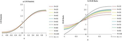
First, we conduct the simulation experiments for LM statistic and ELR ratio in MA (1) model as a function of fixed parameter $\theta$ and different values of N with $m={10}^5$ simulations. Table 2 presents the simulation results of LM statistic and ELR ratio. We find that the value of the LM statistic at $\theta =0$ remains almost same and equals to 1.00 for N =$\left\{10,20,..100,\mathrm{\infty }\right\}$ steps. In case of the ELR ratio, at $\theta =0$, the value of the ELR ratio increases from 1.59 to 2.00 as the number of steps increases from N = 10 to N = $\mathrm{\infty }$. Also we observe that the value of LM statistic and the ELR ratio increases as the fixed parameter $\theta$ increases from $\theta$ = −1 to +1 at each N steps.

Table 2. LM statistic and the ELR ratio in the MA (1) model as a function of fixed parameter $\theta$ and N with m = ${\mathbf{10}}^{\mathbf{5}}$ simulations

	LM statistic											ELR ratio
θ	−1	−0.8	−0.6	−0.4	−0.2	0	0.2	0.4	0.6	0.8	1	−1	−0.8	−0.6	−0.4	−0.2	0	0.2	0.4	0.6	0.8	1
N = 10	0.10	0.12	0.21	0.38	0.66	1.00	1.35	1.63	1.80	1.88	1.91	0.89	0.92	1.02	1.18	1.38	1.59	1.76	1.88	1.95	1.98	1.99
N = 20	0.05	0.07	0.16	0.35	0.64	1.01	1.37	1.67	1.85	1.94	1.96	0.75	0.80	0.95	1.18	1.44	1.70	1.92	2.07	2.16	2.20	2.21
N = 30	0.03	0.06	0.15	0.33	0.63	1.00	1.38	1.68	1.86	1.96	1.98	0.67	0.74	0.92	1.18	1.47	1.76	1.99	2.16	2.25	2.30	2.31
N = 40	0.03	0.05	0.14	0.33	0.63	1.00	1.38	1.67	1.86	1.95	1.97	0.61	0.69	0.90	1.17	1.49	1.79	2.04	2.21	2.31	2.36	2.37
N = 50	0.02	0.04	0.14	0.32	0.62	1.00	1.37	1.67	1.86	1.95	1.98	0.57	0.65	0.87	1.16	1.48	1.80	2.06	2.24	2.35	2.40	2.41
N = 60	0.02	0.04	0.13	0.32	0.62	1.00	1.38	1.67	1.86	1.95	1.98	0.53	0.63	0.86	1.16	1.49	1.82	2.09	2.27	2.38	2.43	2.44
N = 70	0.01	0.04	0.13	0.32	0.62	1.00	1.38	1.68	1.87	1.97	1.99	0.50	0.61	0.85	1.15	1.50	1.83	2.10	2.29	2.41	2.46	2.47
N = 80	0.01	0.04	0.13	0.32	0.63	1.01	1.40	1.70	1.89	1.98	2.01	0.48	0.59	0.84	1.16	1.51	1.85	2.13	2.32	2.43	2.49	2.50
N = 90	0.01	0.04	0.13	0.32	0.62	1.00	1.38	1.68	1.87	1.96	1.99	0.46	0.58	0.83	1.15	1.51	1.85	2.14	2.34	2.45	2.51	2.52
N = 100	0.01	0.03	0.13	0.32	0.62	1.00	1.39	1.69	1.88	1.97	2.00	0.44	0.57	0.82	1.15	1.51	1.86	2.15	2.34	2.46	2.52	2.53
N = ∞	0.00	0.02	0.12	0.31	0.62	1.00	1.38	1.69	1.88	1.98	2.00	0.00	0.31	0.69	1.11	1.57	2.00	2.35	2.60	2.74	2.81	2.83

Figure (2.a) shows that there is an increasing and nonlinear relationship between LM statistic and fixed parameter $\theta$ in the MA (1) model. The impact of increasing the steps N is not felt strongly because the curves for different values of N lie more or less on top of each other. Figure (2.b) displays the relationship between the ELR ratio and fixed parameter $\theta$ in MA (1) model. We can see that for every fixed N, the ELR ratio is increasing with respect to $\theta$, although in a nonlinear fashion. Furthermore, this monotone curve becomes steeper as N increases. Therefore, based on the simulation experiments, when we consider the fixed parameter $\theta$ in the MA (1) model, conditionally both LM statistic and ELR ratio show that there is an increasing and nonlinear relationship.

Figure 2. LM statistic and ELR ratio in the MA (1) model for different values of N and fixed parameter $\theta$.

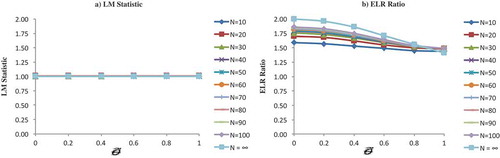
Second, we conduct the simulation experiments for LM statistic and ELR ratio in MA (1) model as a function of stochastic parameter $\tilde{\theta }$ and different values of $N$ with $m={10}^5$ simulations. Table 3 presents the simulation results of LM statistic and ELR ratio. We find that the value of the LM statistic almost exactly equals to 1.00 for each setting of the stochastic parameter $\tilde{\theta }=\{0,0.2,0.4,0.6,0.8,1.00\}$ and for $N$ = $\left\{10,20,..100,\mathrm{\infty }\right\}$ steps. However, in case of the ELR ratio, we observe that the value of ELR ratio decreases as the stochastic parameter $\tilde{\theta }$ increases from 0 to 1.00 at each $N$ steps.

Table 3. LM statistic and the ELR ratio in the MA (1) model as functions of stochastic parameter $\tilde{\theta }$ and $N$ with $m={10}^5$ simulations

	LM statistic						ELR ratio
θ	0	0.2	0.4	0.6	0.8	1	0	0.2	0.4	0.6	0.8	1
N = 10	1.00	1.00	1.00	1.00	1.00	1.00	1.59	1.57	1.53	1.49	1.45	1.44
N = 20	1.01	1.01	1.01	1.01	1.01	1.01	1.70	1.68	1.62	1.55	1.50	1.48
N = 30	1.00	1.00	1.00	1.01	1.01	1.01	1.76	1.73	1.67	1.59	1.52	1.49
N = 40	1.00	1.00	1.00	1.00	1.00	1.00	1.79	1.76	1.69	1.60	1.53	1.49
N = 50	1.00	1.00	1.00	1.00	1.00	1.00	1.80	1.77	1.70	1.61	1.53	1.49
N = 60	1.00	1.00	1.00	1.00	1.00	1.00	1.82	1.79	1.72	1.62	1.53	1.49
N = 70	1.00	1.00	1.00	1.00	1.00	1.00	1.83	1.80	1.72	1.63	1.53	1.49
N = 80	1.01	1.01	1.01	1.01	1.01	1.01	1.85	1.82	1.74	1.64	1.54	1.49
N = 90	1.00	1.00	1.00	1.00	1.00	1.00	1.85	1.82	1.74	1.64	1.54	1.49
N = 100	1.00	1.00	1.00	1.00	1.00	1.00	1.86	1.83	1.75	1.64	1.54	1.49
N = ∞	1.00	1.00	1.00	1.00	1.00	1.00	2.00	1.96	1.86	1.71	1.56	1.41

Figure (3.a) shows that LM statistic remains to be equal to its bootmean value 1 irrespective of the value of the stochastic parameter $\tilde{\theta }$ in the MA (1) model. It is for this reason the LM statistic will not be able to detect the presence of mean reversion as the LM statistic will always be equal to its bootmean value. Figure (3.b) displays the relationship between the ELR ratio and stochastic parameter $\tilde{\theta }$ in the MA (1) model. We can see that for every fixed N, the ELR ratio is decreasing with respect to $\tilde{\theta }$, although in a nonlinear fashion. Therefore, based on the simulation experiments, when we consider the stochastic parameter $\tilde{\theta }$ in the MA (1) model, unconditionally LM statistic is always equal to its bootmean value whereas ELR ratio is decreasing with respect to $\tilde{\theta }$ in a nonlinear fashion.

Figure 3. LM statistic and ELR ratio in the MA (1) model for different values of $N$ and stochastic parameter $\tilde{\theta }$.

Third, in Table (4.a), we present the deviation of LM statistic and ELR ratio from their respective bootmeans in fixed parameter MA (1) model for different values of $N$, i.e., for $\left\{N=10,N=100,N=\mathrm{\infty }\right\}$. We find that when the MA parameter $\theta$ is negative, the deviation of the LM statistic and ELR ratio from their respective bootmeans is also negative. Similarly, we find that when the MA parameter $\theta$ is positive, the deviation of the LM statistic and ELR ratio from their respective bootmeans is also positive. Figure (4.a) shows the plot between deviation of LM statistic from its bootmean on X-axis with respect to the deviation of ELR ratio from its bootmean on Y-axis. It shows that when LM statistic is negative, ELR ratio is also negative and vice versa. It shows the nonlinear relationship between the two and the impact gets only stronger as the value of N increases from N = 10 to $N=\mathrm{\infty }$. Furthermore, in Table (4.b), we present the deviation of LM statistic and ELR ratio from their respective bootmean in stochastic parameter MA (1) model for different values of N, i.e., for $\left\{N=10,N=100,N=\mathrm{\infty }\right\}$. We find that there is no deviation of LM statistic from its bootmean in case of stochastic parameter for different values of N in MA (1) model. The deviation of ELR ratio from its bootmean is negative and its impact increases as the value of N moves from N = 10 to $N=\mathrm{\infty }$. Figure (4.b) shows the plot between deviation of LM statistic and ELR ratio from its bootmean for different values of N, i.e., for $\left\{N=10,N=100,N=\mathrm{\infty }\right\}$ in case of stochastic parameter MA (1) model. It shows that deviation of ELR ratio from its bootmean increases from N = 10 to N = $\mathrm{\infty }$ even though when there is no deviation of LM statistic from its bootmean.

Figure 4. Deviation of LM statistic and the ELR ratio from their respective bootmean in the MA (1) model as a function of fixed/stochastic parameter for different values of N, i.e., for N = 10, N = 100 and $\mathit{N}=$∞.

4. Empirical work

4.1. Data description

Our data set consists of the daily (opening, high, low, and closing) prices of the constituents of the BSE SENSEX, which is a free float market weighted Indian stock market index. It comprises of 30 most actively traded companies listed on the Bombay Stock Exchange, also called as BSE 30.

We collect the daily data of 22 constituent stocks⁶ of BSE SENSEX for the overall sample period from January 2001 to September 2015 (3671 daily observations). The reason for selecting only 22 stocks of SENSEX index out of 30 constituent stocks is twofold. First, to keep the daily observations of the panel, data of constituent stocks of the SENSEX index remain same across different sample periods to avoid the impact of the companies which leave or join the index in our empirical work. Second, the unavailability of open, high, low, and close price series data during different sample periods for all the constituent stocks of the index. Because of the above-mentioned reasons, we have cleaned the data and selected the panel data of 22 constituent stocks which remain same across different sample periods so that we can compare our empirical findings based on two different test statistics.

The daily data are collected from the source: Bloomberg. Table 5 shows the descriptive statistics of the daily return series⁷ of 22 individual stocks of BSE SENSEX. We observe that 12 out of 22 stocks are negatively skewed. The average mean return and standard deviation of the individual 22 stocks are 0.0007 and 0.0240, respectively.

Table 4. Deviation of LM statistic and the ELR ratio from their respective bootmean in the MA (1) model as a function of fixed/stochastic parameter for different values of N

	a) Fixed parameter								b) Stochastic parameter
	N = 10		N = 100		N = ∞			$\tilde{\theta }$	N = 10		N = 100		N = ∞
θ	LM	ELR	LM	ELR	LM	ELR			LM	ELR	LM	ELR	LM	ELR
−1	−0.90	−0.70	−0.99	−1.41	−1.00	−2.00		0	0.00	0.00	0.00	0.00	0.00	0.00
−0.8	−0.88	−0.67	−0.97	−1.29	−0.98	−1.69		0.2	0.00	−0.02	0.00	−0.03	0.00	−0.04
−0.6	−0.80	−0.57	−0.88	−1.04	−0.88	−1.31		0.4	0.00	−0.06	0.00	−0.11	0.00	−0.14
−0.4	−0.62	−0.40	−0.69	−0.71	−0.69	−0.89		0.6	0.00	−0.10	0.00	−0.22	0.00	−0.29
−0.2	−0.35	−0.20	−0.38	−0.35	−0.38	−0.43		0.8	0.00	−0.14	0.00	−0.32	0.00	−0.44
0	0.00	0.00	0.00	0.00	0.00	0.00		1	0.00	−0.15	0.00	−0.37	0.00	−0.59
0.2	0.35	0.17	0.38	0.29	0.38	0.35
0.4	0.62	0.29	0.69	0.49	0.69	0.60
0.6	0.80	0.36	0.88	0.60	0.88	0.74
0.8	0.88	0.39	0.97	0.66	0.98	0.81
1	0.90	0.40	0.99	0.67	1.00	0.83

The bold values represents the fixed/stochastic parameter.

Table 5. Descriptive statistics of the 22 individual BSE SENSEX stocks

S.no	Stock	Mean		Standard Error	Median	Standard Deviation	Kurtosis	Skewness	Range	Minimum	Maximum
1	AXIS	0.0011	0.0	0.0005	0.0000	0.0292	4.1621	0.3360	0.3640	−0.1788	0.1852
2	BHEL	0.0007	0.0	0.0004	0.0003	0.0260	6.0517	−0.1240	0.4231	−0.2272	0.1959
3	CIPLA	0.0006	0.0	0.0003	0.0001	0.0193	5.0529	−0.2418	0.2581	−0.1540	0.1040
4	DRRD	0.0007	0.0	0.0003	0.0007	0.0201	8.1642	−0.2534	0.3617	−0.2008	0.1610
5	GAIL	0.0006	0.0	0.0004	0.0001	0.0234	13.8683	−0.0735	0.5234	−0.2395	0.2839
6	HDFC	0.0008	0.0	0.0004	0.0002	0.0229	4.8453	0.3963	0.3075	−0.1173	0.1903
7	HDFCB	0.0009	0.0	0.0003	0.0003	0.0196	4.0726	0.2424	0.2713	−0.1195	0.1518
8	HMCL	0.0007	0.0	0.0004	0.0000	0.0220	3.6912	0.4363	0.2577	−0.0922	0.1654
9	HNDL	0.0000	0.0	0.0004	0.0004	0.0267	3.5992	−0.1522	0.3638	−0.1963	0.1676
10	HUVR	0.0004	0.0	0.0003	−0.0001	0.0187	5.1130	0.2374	0.3221	−0.1627	0.1594
11	ICICI	0.0006	0.0	0.0005	0.0000	0.0276	5.1616	0.0193	0.4267	−0.2196	0.2071
12	INFO	0.0005	0.0	0.0004	0.0004	0.0241	15.5132	−1.0062	0.4679	−0.3117	0.1562
13	ITC	0.0006	0.0	0.0003	0.0004	0.0187	3.3187	−0.0378	0.2159	−0.1106	0.1052
14	MM	0.0009	0.0	0.0004	0.0007	0.0247	4.6540	0.0275	0.3826	−0.1748	0.2078
15	ONGC	0.0007	0.0	0.0004	0.0000	0.0229	6.0129	0.2263	0.3450	−0.1626	0.1823
16	RIL	0.0006	0.0	0.0004	0.0006	0.0228	29.0544	1.2279	0.5722	−0.1796	0.3926
17	SBIN	0.0007	0.0	0.0004	0.0008	0.0234	3.9049	−0.0647	0.3440	−0.1597	0.1843
18	SUNP	0.0012	0.0	0.0003	0.0005	0.0203	4.0477	−0.1025	0.2592	−0.1619	0.0973
19	TATA	0.0003	0.0	0.0005	0.0004	0.0281	3.4028	−0.2836	0.3167	−0.1641	0.1526
20	TTMT	0.0008	0.0	0.0005	0.0006	0.0275	3.3502	−0.1111	0.3560	−0.1810	0.1750
21	VEDL	0.0011	0.0	0.0006	0.0000	0.0334	3.4067	0.2880	0.4392	−0.2508	0.1884
22	WPRP	0.0003	0.0	0.0004	0.0004	0.0268	8.3386	−0.2622	0.4045	−0.2029	0.2016

Total daily observations of each stock is 3671 from January 01, 2001 to September 24, 2015.

Table 6. Empirical analysis of LM statistic and ELR ratio on cross-sectional average of BSE SENSEX using bootstrap method in the overall sample period (January 2001 to September 2015)

a) LM statistic
k-day	1	2	3	4	5	6	7	8	9	10	11	12	13	14	15	16	17	18	19	20
Actual LM	1	1.04	1.03	1.01	0.99	0.98	0.96	0.95	0.95	0.94	0.94	0.94	0.94	0.94	0.94	0.95	0.95	0.95	0.95	0.95
Boot LM (Boot s.e)	1	1.00	1.00	1.00	1.00	1.00	1.00	1.00	1.00	1.00	1.00	1.00	1.00	1.00	1.00	1.00	1.00	0.99	0.99	1.00
	(0.00)	(0.02)	(0.02)	(0.03)	(0.04)	(0.04)	(0.04)	(0.05)	(0.05)	(0.06)	(0.06)	(0.06)	(0.06)	(0.07)	(0.07)	(0.07)	(0.07)	(0.08)	(0.08)	(0.08)
t-stat	N/A	2.45*	1.16	0.26	−0.14	−0.49	−0.80	−0.94	−0.97	−0.96	−0.91	−0.87	−0.85	−0.82	−0.76	−0.69	−0.66	−0.61	−0.56	−0.52
Degrees of freedom	N/A	19	18	17	16	15	14	13	12	11	10	9	8	7	6	5	4	3	2	1
GMM stat (p-value)	N/A	17.89 (0.53)	11.44 (0.87)	10.12 (0.90)	10.08 (0.86)	10.04 (0.82)	9.73 (0.78)	9.18 (0.76)	7.98 (0.79)	6.78 (0.82)	5.67 (0.84)	4.83 (0.85)	4.04 (0.85)	3.46 (0.84)	2.63 (0.85)	2.03 (0.85)	1.45 (0.83)	0.97 (0.81)	0.61 (0.74)	0.26 (0.61)
b) ELR ratio
k-day	1	2	3	4	5	6	7	8	9	10	11	12	13	14	15	16	17	18	19	20
Actual LM	1	1.04	1.05	1.06	1.07	1.08	1.08	1.08	1.08	1.09	1.09	1.09	1.09	1.09	1.09	1.09	1.09	1.10	1.10	1.10
Boot LM (Boot s.e)	1	1.08	1.11	1.13	1.15	1.16	1.16	1.17	1.18	1.18	1.18	1.19	1.19	1.19	1.19	1.19	1.19	1.20	1.20	1.20
	(0.00)	(0.00)	(0.01)	(0.01)	(0.01)	(0.01)	(0.01)	(0.01)	(0.01)	(0.02)	(0.02)	(0.02)	(0.02)	(0.02)	(0.02)	(0.02)	(0.02)	(0.02)	(0.02)	(0.02)
t-stat	N/A	−10.16**	−9.15**	−8.35**	−7.92**	−7.39**	−6.91**	−6.62**	−6.30**	−6.09**	−5.86**	−5.69**	−5.47**	−5.31**	−5.12**	−4.97**	−4.88**	−4.71**	−4.57**	−4.48**
Degrees of freedom	N/A	19	18	17	16	15	14	13	12	11	10	9	8	7	6	5	4	3	2	1
GMM stat (p-value)	N/A	804.13** (0.00**)	728.98** (0.00**)	626.14** (0.00**)	569.71** (0.00**)	489.16** (0.00**)	441.63** (0.00**)	397.86** (0.00**)	352.32** (0.00**)	314.82** (0.00**)	273.32** (0.00**)	238.43** (0.00**)	203.64** (0.00**)	167.43** (0.00**)	138.93** (0.00**)	112.54** (0.00**)	91.54** (0.00**)	61.41** (0.00**)	38.25** (0.00**)	17.50** (0.00**)

$\ast \ast ,\ast$ represent level of significance at $1\mathrm{\%},5\mathrm{\%}$, respectively.

Table 7. Empirical analysis of LM statistic and ELR ratio on cross-sectional average of BSE SENSEX using bootstrap method in the pre-crisis sample period

	Pre-crisis period (January 2001 to December 2007)									a) LM statistic
k-day	1	2	3	4	5	6	7	8	9	10	11	12	13	14	15	16	17	18	19	20
Actual LM	1	1.03	1.00	0.98	0.97	0.96	0.95	0.94	0.93	0.93	0.93	0.93	0.93	0.93	0.93	0.93	0.93	0.93	0.93	0.93
Boot LM (Boot s.e)	1	1.00	1.00	1.00	1.00	1.00	1.00	1.00	1.00	0.99	0.99	0.99	0.99	0.99	0.99	0.99	0.99	0.99	0.99	0.99
	(0.00)	(0.02)	(0.04)	(0.04)	(0.05)	(0.06)	(0.07)	(0.07)	(0.08)	(0.08)	(0.08)	(0.09)	(0.09)	(0.10)	(0.10)	(0.10)	(0.11)	(0.11)	(0.11)	(0.12)
t-stat	N/A	1.44	0.17	−0.40	−0.51	−0.58	−0.69	−0.80	−0.87	−0.83	−0.76	−0.71	−0.71	−0.67	−0.62	−0.59	−0.57	−0.55	−0.52	−0.50
Degrees of freedom	N/A	19	18	17	16	15	14	13	12	11	10	9	8	7	6	5	4	3	2	1
GMM		10.40	7.57	7.50	7.27	7.07	6.80	6.27	5.58	4.75	4.16	3.41	2.84	2.28	1.82	1.39	1.13	0.81	0.51	0.25
		(0.94)	(0.98)	(0.98)	(0.97)	(0.96)	(0.94)	(0.94)	(0.94)	(0.94)	(0.94)	(0.95)	(0.94)	(0.94)	(0.94)	(0.93)	(0.89)	(0.85)	(0.77)	(0.61)
	Pre-crisis period (January 2001 to December 2007)									b) ELR ratio
k-day	1	2	3	4	5	6	7	8	9	10	11	12	13	14	15	16	17	18	19	20
Actual ELR	1	1.04	1.06	1.07	1.07	1.08	1.08	1.09	1.09	1.09	1.09	1.09	1.10	1.10	1.10	1.10	1.10	1.10	1.10	1.10
Boot ELR (Boot s.e)	1 (0.00)	1.08 (0.01)	1.12 (0.01)	1.14 (0.01)	1.16 (0.01)	1.17 (0.02)	1.18 (0.02)	1.18 (0.02)	1.19 (0.02)	1.19 (0.02)	1.20 (0.02)	1.21 (0.02)	1.21 (0.03)	1.21 (0.03)	1.21 (0.03)	1.21 (0.03)	1.21 (0.03)	1.21 (0.03)	1.21 (0.03)	1.21 (0.03
t-stat	N/A	−7.50**	−6.95**	−6.38**	−6.01**	−5.72**	−5.40**	−5.20**	−4.98**	−4.78**	−4.63**	−4.44**	−4.24**	−4.09**	−4.00**	−3.87**	−3.73**	−3.60**	−3.52**	−3.45**
Degrees of freedom	N/A	19	18	17	16	15	14	13	12	11	10	9	8	7	6	5	4	3	2	1
GMM	N/A	487.77** (0.00**)	432.78** (0.00**)	387.04** (0.00**)	336.34** (0.00**)	296.7** (0.00**)	264.59** (0.00**)	229.99** (0.00**)	202.42** (0.00**)	175.24** (0.00**)	152.56** (0.00**)	132.24** (0.00**)	114.47** (0.00**)	98.82** (0.00**)	83.29** (0.00**)	64.72** (0.00**)	48.96** (0.00**)	35.15** (0.00**)	23.81** (0.00**)	11.61** (0.00**)

**,* represent the level of significance at 1% and 5% respectively.

Table 8. Empirical analysis of LM statistic and ELR ratio on cross-sectional average of BSE SENSEX using bootstrap method in the post-crisis sample period

k-day	1	2	3	4	5	6	7	8	9	10	11	12	13	14	15	16	17	18	19	20
Actual LM	1.00	1.04	1.04	1.03	1.01	0.98	0.96	0.95	0.95	0.94	0.94	0.94	0.94	0.94	0.94	0.94	0.94	0.94	0.94	0.94
Boot LM (Boot s.e)	1.00	1.00	1.00	1.00	1.00	1.00	1.00	1.00	1.00	1.00	0.99	0.99	0.99	0.99	0.99	0.99	0.99	0.99	0.99	0.99
	(0.00)	(0.02)	(0.03)	(0.04)	(0.05)	(0.06)	(0.06)	(0.07)	(0.07)	(0.08)	(0.08)	(0.09)	(0.09)	(0.09)	(0.10)	(0.10)	(0.10)	(0.11)	(0.11)	(0.11)
t-stat	N/A	1.87	1.30	0.64	0.17	−0.24	−0.57	−0.66	−0.65	−0.66	−0.65	−0.64	−0.60	−0.60	−0.57	−0.57	−0.53	−0.50	−0.46	−0.43
Degrees of freedom	N/A	19	18	17	16	15	14	13	12	11	10	9	8	7	6	5	4	3	2	1
GMM		10.64	7.20	5.39	4.94	4.91	4.83	4.39	3.96	3.57	3.13	2.79	2.34	2.07	1.59	1.26	0.90	0.63	0.39	0.19
	N/A	(0.94)	(0.99)	(0.99)	(0.99)	(0.99)	(0.99)	(0.99)	(0.98)	(0.98)	(0.98)	(0.97)	(0.97)	(0.96)	(0.95)	(0.94)	(0.92)	(0.89)	(0.82)	(0.66)
k-day	1	2	3	4	5	6	7	8	9	10	11	12	13	14	15	16	17	18	19	20
Actual ELR	1.00	1.03	1.05	1.06	1.07	1.07	1.07	1.08	1.08	1.08	1.08	1.08	1.08	1.09	1.09	1.09	1.09	1.09	1.09	1.09
Boot ELR (Boot s.e)	1.00	1.07	1.09	1.11	1.12	1.13	1.13	1.14	1.14	1.14	1.15	1.15	1.15	1.15	1.15	1.15	1.15	1.15	1.15	1.15
	(0.00)	(0.01)	(0.01)	(0.01)	(0.01)	(0.01)	(0.02)	(0.02)	(0.02)	(0.02)	(0.02)	(0.02)	(0.02)	(0.03)	(0.03)	(0.03)	(0.03)	(0.03)	(0.03)	(0.03)
t-stat	N/A	−5.91**	−5.06**	−4.50**	−4.12**	−3.82**	−3.54**	−3.33**	−3.16**	−3.04**	−2.89**	−2.79**	−2.67**	−2.56**	−2.50**	−2.42**	−2.38**	−2.32**	−2.29**	−2.27**
Degrees of freedom	N/A	19	18	17	16	15	14	13	12	11	10	9	8	7	6	5	4	3	2	1
GMM		246.22**	197.50**	168.50**	142.50**	120.62**	107.79**	96.21**	82.09**	68.72**	60.47**	52.93**	43.44**	37.73**	31.10**	26.14**	20.37**	15.10**	10.15**	5.04*
		(0.00**)	(0.00**)	(0.00**)	(0.00**)	(0.00**)	(0.00**)	(0.00**)	(0.00**)	(0.00**)	(0.00**)	(0.00**)	(0.00**)	(0.00**)	(0.00**)	(0.00**)	(0.00**)	(0.00**)	(0.01**)	(0.02*)

**,* represent the level of significance at 1% and 5% respectively.

Table 9. Scatterplot of the deviation of CS average of LM statistic and ELR ratio from its bootmean in the pre-crisis period and post-crisis period for k-day = 10 and k-day = 20 {fig a, fig b, fig c, fig d}. Scatterplot of the deviation of actual ELR and actual theta from the CS average of BSE SENSEX in the pre-crisis and post-crisis period {fig e, fig f}.

4.2. Findings of overall sample period

(January 2001 to September 2015):

We perform the empirical test on the Indian stock market by considering the daily data of BSE SENSEX for the overall sample period from January 2001 to September 2015.

4.2.1. LM statistic

Table (6.a) shows the CS average of the LM statistic values for horizons up to k-day = 20. We can find that if we were to consider each k-day separately, we can reject the random walk hypothesis for k-day = 2, because the individual t-statistic is significant at 95% level of confidence and is equal to 2.45. Since the value of CS average of actual LM statistic is 1.04 at k-day = 2, it supports momentum in the stock market but not mean reversion. In addition, we report the values of the generalized method of momemts (GMM) statistic as per Richardson & Smith.T. (1991) for the joint hypothesis that the CS average of the LM statistic is equal to its bootstrap mean for all lags from the k-day = 1 to k-day = 20. We display the p-value, i.e., the right tail probability of the GMM ${\chi }^2$ statistic for testing the joint hypothesis across different k-days. We observe that p-values across different k-days are insignificant, and hence, we cannot reject the random walk hypothesis, or that returns are independent over time, for lag more than 2. Thus, if we were to go by the LM statistic, then we cannot find any evidence of mean reversion in asset prices for the overall sample period from January 2001 to September 2015. Also, Figure (5.a) justifies the argument we have made based on the evidence from Table (6.a). That is, the CS average of the LM statistic for different k-days all resides within the range of the 95% confidence interval.

Figure 5. LM statistic and ELR ratio on cross-sectional (CS) average of BSE SENSEX with $\mathbf{95}\mathbf{\%}$ confidence interval in the overall sample period (January 2001 to September 2015).

4.2.2. ELR ratio

In Table (6.b), we report the CS average of the ELR ratio for horizons from k-day = 1–20 for the combined sample period from January 2001 to September 2015. We can find that all the individual t-statistics are highly significant at 99% level of confidence and so are the GMM ${\chi }^2$ statistics based on the joint hypothesis test. Thus, we can reject null hypothesis of random walk by individual t-statistics. Also we can reject the null hypothesis that CS average of the ELR ratio is equal to its bootmean based on the joint GMM ${\chi }^2$ statistic. Furthermore, the sign is negative for all individual t-test statistics, which shows evidence of mean reversion in the Indian stock market. We observe that the CS average of the actual ELR ratio is much less than its bootstrap mean across different k-days indicating the presence of mean reversion. The CS average of ELR ratio and its 95% confidence interval are shown in Figure (5.b), where it is evident that the deviation from the bootstrap mean lies wholly outside the 95% confidence band. Thus, from both Table (6.b) and Figure (5.b), we see that there is no ambiguity in rejecting the random walk hypothesis in favor of mean reversion in the Indian BSE SENSEX using the CS average of the ELR ratio.

4.2.3. Comparitive analysis

We have shown so far that it is possible for the CS average of the LM statistic to be equal to unity which is its bootstrap mean, while the CS average of the ELR ratio to be less than its bootstrap mean, when mean reversion is present in the MA (1) model. Therefore, we argue that ELR ratio is superior to the traditional LM statistic when it comes to detecting mean reversion, such as what we find to be in the case of India’s BSE SENSEX.

To study the relationship between the ELR ratio and the LM statistic in the data, we computed the deviation of the ELR ratio and the LM statistic from their respective bootmean for each individual company of BSE SENSEX. The scatterplot of LM statistic and ELR ratios from their respective bootmeans for k-day = 10 and k-day = 20 in Figure 6 display that there is a nonlinear relationship in the data as expected as in Figure (4.a). The curvature of the scatterplot of the deviation of ELR ratio versus that of the LM statistic is more pronounced in the case of k-day = 20.

Figure 6. Scatterplot of LM atatistic and ELR ratio from its bootmean for k-day = 10 and k-day = 20 in the combined sample.

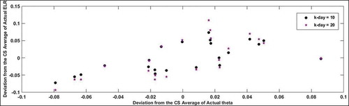
In addition, we estimated the $\theta$ parameter in the MA (1) model for each individual 22 stocks under consideration in India’s BSE SENSEX using the first order autocorrelation of close-to-close returns. In Figure 7, we plot the relationship between the deviation from the CS average of actual $\theta$ and that of actual ELR ratio for the combined sample for k-day = 10 and k-day = 20. We can see that the left of zero in the horizontal axis, the star symbol (*) representing k-day = 20 stays below that of the circle representing k-day = 10. Similarly to the right of the horizontal axis, the star symbol (*) representing k-day = 20 stays above that of the circle representing k-day = 10. This is exactly what we expect to see in the data as per our ELR ratio in the MA (1) model for different values of N and fixed parameter $\theta$ as shown in Figure 2. Thus, we say that MA (1) model is well suited for the data and the ELR ratio is capable of detecting mean reversion in the India’s BSE SENSEX much better when compared to the traditional LM statistic.

Figure 7. Scatterplot of ELR ratio and $\theta$ for k-day = 10 and k-day = 20 in the combined sample.

5. Robustness check

In this section, we undertake a check on the robustness of our findings by analyzing sub-samples from before and after the global financial crisis of 2008. Specifically, we split the combined sample of 2001–2015 into sub-sample 1 based on data from January 2001 to December 2007 (1756 daily observations) and sub-sample 2 from January 2008 to September 2015 (1919 daily observations). We performed all the analysis similar to what we have done for the combined sample.

5.1. Pre-crisis period (January 2001 to December 2007)

Table (7.a) presents CS average of the LM statistic in sub-sample 1 (2001–2007). We find that we cannot reject the random walk hypothesis based on the individual t-stat values and the GMM stat values. The CS average of the LM statistic and its 95% confidence interval are shown in Figure (8.a), where it is evident that the deviation from the bootstrap mean lies within the 95% confidence band. Thus, if we were to go by the CS average of the LM statistic, we cannot find any evidence of mean reversion in asset prices during the pre-crisis period from January 2001 to December 2007.

Figure 8. LM statistic and ELR ratio on CS average of BSE SENSEX with $95\mathbf{\%}$ confidence interval in the pre-crisis period (January 2001 to December 2007).

In Table (7.b), we report the CS average of the ELR ratio for horizons up to k-day = 20. We can see from the table that all the individual tstatistics are highly significant and so are the GMM ${\chi }^2$ statistics based on the joint hypothesis test. Thus, based on the individual t-test statistics, we reject the random walk hypothesis using the ELR ratio for the pre-crisis period (2001–2007). Thus, from both Table (7.b) and Figure (8.b), we see that there is no ambiguity in rejecting the random walk hypothesis in favor of mean reversion in the Indian BSE SENSEX in the pre-crisis sample period using the CS average of the ELR ratio.

In addition, the scatterplot of CS average of the LM statistic and ELR ratios from their respective bootmeans for k-day = 10 and k-day = 20 displays that there is a nonlinear relationship in the data as shown in Table (9.a, 9.b). In Table (9.e), we plot the relationship between the deviation from the CS average of actual $\theta$ and that of actual ELR ratio for the sub-sample for k-day = 10 and k-day = 20. We find that MA (1) is well suited and ELR ratio is able to detect mean reversion in the pre-crisis period even though the LM statistic is not able to do so.

5.2. Crisis and post-crisis period

(January 2008 to September 2015)

Based on the empirical results shown in Table (8.a) and Figure (9.a), we can clearly say that we cannot find any evidence of mean reversion as per the CS average of the LM statistic in the sub-sample period from January 2008 to September 2015. However, we can show that their is enough evidence of mean reversion in the crisis and post-crisis period as per the CS average of the ELR ratio, based on the significant individual t-stat values and the joint hypothesis GMM stat values as in Table (8.b) and also as per Figure (9.b).

Figure 9. LM statistic and ELR ratio on CS average of BSE SENSEX with $\mathbf{95}\mathbf{\%}$ confidence interval in the post-crisis period (January 2008 to September 2015).

In addition, the scatterplot of CS average of the LM statistic and ELR ratios from their respective bootmeans for k-day = 10 and k-day = 20 displays that there is a nonlinear relationship in the data as shown in Table (9.c, 9.d) in the post-crisis sample period. In Table (9.f), we plot the relationship between the deviation from the CS average of actual $\theta$ and that of actual ELR ratio for the sub-sample for k-day = 10 and k-day = 20. We find that MA (1) is well suited and CS average ELR ratio in BSE SENSEX is able to detect mean reversion in the post-crisis period.

6. Conclusion

The presence of mean reversion makes the stocks less risky which can have an important economic implications especially for long time investors. In this article, we use the ELR ratio based on high and low prices, and test for the presence of mean reversion. We show that the proposed ELR ratio is superior in detecting the presence of mean reversion when compared to the traditional Lo and MacKinlay (1988) test statistic. We prove the superiority theoretically using simulations and also test the same empirically by way of the CS average of the constituent stocks of the BSE sensex index.

Using Monte Carlo simulation experiments, we show that there is a deep connection between the degree of mean reversion and the ELR ratio. Especially, we have found that when we consider the fixed parameter $\theta$ in the MA (1) model, conditionally both the traditional Lo and MacKinlay (1988) statistic and the ELR ratio show that there is an increasing and nonlinear relationship. However, when we consider the stochastic parameter $\tilde{\theta }$ in the MA (1) model, we found that ELR ratio decreases whereas the LM statistic remains flat.

We have shown in the data that the actual CA average of the ELR ratio is significantly less than its bootstrap mean, indicating there is a considerable amount of mean reversion. Whereas, the actual CS average of the LM statistic proposed by Lo and MacKinlay (1988), based on closing prices alone, is almost exactly equal to its bootstrap mean, which would ordinarily be taken to imply that there is no mean reversion.

The empirical analysis is carried out in three different sample periods, i.e., from 2001 to 2015 (overall sample period), from 2001 to 2007 (pre-crisis period), and from 2008 to 2015 (crisis and post-crisis period). The idea to choose three different sample periods is for checking the robustness of our results across different sample periods based on two different test statistics, i.e., ELR and LM statistic. It is important to note that the CS average of ELR ratio is able to detect mean reversion in not just the crisis and post-crisis period from 2008 to 2015 but also during the pre-crisis period from 2001 to 2007 and also during the overall period from 2001 to 2015. However, the LM statistic fails to find the evidence of mean reversion during all the three different sample periods. Therefore, we argue that ELR ratio is superior and more conclusive in detecting the presence of mean reversion when compared to the LM statistic.

The analysis is not just restricted to the constituent stocks of any index but it can be replicated to other individual stock indices and other asset classes such as currency pairs and precious metals in future research to detect the presence of mean reversion. Further, we can also conduct analysis in other emerging and developed markets to detect the presence of mean reversion using the ELR ratio.

Additional information

Funding

The authors received no direct funding for this research.

Notes on contributors

Muneer Shaik

Muneer Shaik is a Faculty Associate at Institute for Financial Management and Research (IFMR), Chennai India. He holds PhD in finance at IFMR. He worked with J.P.Morgan in a managerial position in the equity and fixed income department. He has participated and presented his research papers at multiple conferences both in India and abroad. Some of his research papers have won the best paper awards. His research interests mainly include in the areas of volatility modeling, financial econometrics, and market efficiency.

Notes

1. The most commonly used unit root tests include augmented Dickey–Fuller test (Dickey and Fuller, 1979) and Phillips–Perron test (Phillips and Perron, 1988).

2. Some other tests to detect the random walk hypothesis include Chow and Denning (1993), Wright (2000), ARIMA, and GARCH tests.

3. Turan et al. (2008) investigate the predictive power of the extreme daily returns observed in a fixed time interval.

4. We perform the bootstrap alaysis as per Efron and Tibshirani (1986).

5. We use Spitzer’s identity to show the random walk effect in ELR ratio in Appendix A.

6. The 8 stocks that were excluded are BHARTI, BJAUT, COAL, LPC, LT, MSIL, NTPC, and TCS.

7. The daily returns are calculated from the daily closing prices of the individual stocks using the standard formula: rt = log(Pt/Pt−1) where Pt and Pt−1 are the closing prices on days t and t − 1, respectively.

Appendix A

Spitzer’s identity for the maximum of a random walk is given by

(8) $\mathbb{E}(M_N)=\sum _{k=1}^N\frac{1}{k}\mathbb{E}(S_k^{+})$(8)

where $M_N=max(S_n:0\le n\le N)$ and $S_k^{+}=max(0,S_k)$.

Since we are interested in the range of a random walk, i.e., $R_N=M_N-m_N$, we can modify the identity as,

(9) $\begin{array}{cc}\mathbb{E}(R_N)& =\sum _{k=1}^N\frac{1}{k}[\mathbb{E}(S_k^{+})+\mathbb{E}(S_k^{-})]\\ \hspace{0.17em}& =\sum _{k=1}^N\frac{1}{k}\mathbb{E}\left|S_k\right|\end{array}$(9)

where $S_k\sim N(\mu k,k)$. From above equation (8), we have

(10) $\begin{array}{cc}\mathbb{E}\left|S_k\right|& =\underset{-\mathrm{\infty }}{\overset{\mathrm{\infty }}{\int }}\left|S_k\right|f_{S_k}(S_k)ds\\ \hspace{0.17em}& =\underset{-\mathrm{\infty }}{\overset{0}{\int }}-x_k{f}_X(x)dx+\underset{0}{\overset{\mathrm{\infty }}{\int }}{x}_k{f}_X(x)dx\end{array}$(10)

Part 2 of Equation (10) is given by

(11) $\underset{0}{\overset{\mathrm{\infty }}{\int }}{x}_k{f}_X(x)dx=\mu k\mathrm{\Phi }(\mu \sqrt{k})+\sqrt{k}\phi (\mu \sqrt{k})$(11)

Similarly, Part 1 of Equation (10) is given by

(12) $\underset{-\mathrm{\infty }}{\overset{0}{\int }}-x_k{f}_X(x)dx=-\mu k\mathrm{\Phi }(-\mu \sqrt{k})+\sqrt{k}\phi (\mu \sqrt{k})$(12)

Combining Equations (11) and (12) we get that

(13) $\begin{array}{cc}\mathbb{E}(R_N)& =\mu \sum _{k=1}^N[2\mathrm{\Phi }(-\mu \sqrt{k})-1]\\ \hspace{0.17em}& +2\sum _{k=1}^N[\frac{1}{\sqrt{k}}\phi (\mu \sqrt{k})]\end{array}$(13)

Appendix B8.1. Procedure to compute ELR in data

Let us call $\left\{O_t,H_t,L_t,C_t\right\}$ as the daily $\left\{Open,High,Low,Close\right\}$ prices of an asset at time t, respectively.

Let us define $\left\{x_t,b_t,c_t\right\}$ as below

$x_t=log\left(\frac{C_t}{O_t}\right)$

$b_t=log\left(\frac{H_t}{O_t}\right)$

$c_t=log\left(\frac{L_t}{O_t}\right)$

Now let us define the expected lifetime range (ELR) at time t as

$EL{R}_t=(b-c{)}_t$

We first calculate the one-day ELR as

$ELR{|}_{1day}=\mathbb{E}(b-c){|}_{1day}$

We then calculate the N-day ELR as

$ELR{|}_{Nday}=\mathbb{E}(b-c){|}_{Nday}$

Finally, we find the ELR ratio defined as

(14) $\begin{array}{cc}ELRRatio& =\left\{\frac{1}{\sqrt{N}}\right\}\ast \left\{\frac{ELR{|}_{Nday}}{ELR{|}_{1day}}\right\}\end{array}$(14)

8.2. Procedure to compute LM Statistic in data

We first convert the daily observations of $\left\{Open,High,Low,Close\right\}$ of an asset at time t to $\left\{x_t,b_t,c_t\right\}$ as explained above.

We calculate the LM statistic as below

(15) $\begin{array}{cc}LMStatistic& =\left\{\frac{1}{N}\right\}\ast \left\{\frac{Variance(N-day)}{Variance(1day)}\right\}\end{array}$(15)

References

- Al-Khazali, O. M., Ding, D. K., & Pyun, C. S. (2007). A new variance ratio test of random walk in emerging markets: A revisit. The Financial Review, 42, 303–317. doi:10.1111/fire.2007.42.issue-2
- Bali, T. G., Demirtas, K. O., & Levy, H. (2008). Nonlinear mean reversion in stock prices. Journal of Banking & Finance, 32, 767–782. doi:10.1016/j.jbankfin.2007.05.013
- Caporale, G. M., & Gil-Alana, L. A. (2002). Fractional integration and mean reversion in stock prices. The Quarterly Review of Economics and Finance, 42, 599–609. doi:10.1016/S1062-9769(00)00085-5
- Chaudhuri, K., & Wu, Y. (2004). Mean reversion in stock prices: Evidence from emerging markets. Managerial Finance, 30, 22–37.
- Choi, I., & Chue, T. K. (2007). Subsampling hypothesis tests for nonstationary panels with applications to exchange rates and stock prices. Journal of Applied Econometrics, 22, 233–264. doi:10.1002/(ISSN)1099-1255
- Chow, K. V., & Denning, K. C. (1993). A simple multiple variance ratio test. Journal of Econometrics, 58, 385–401. doi:10.1016/0304-4076(93)90051-6
- Cochrane, J. H. (1988). How big is the random walk in GNP? Journal of Political Economy, 96, 893–920. doi:10.1086/261569
- De Bondt, W. F., & Thaler, R. (1985). Does the stock market overreact? The Journal of Finance, 40, 793–805. doi:10.1111/j.1540-6261.1985.tb05004.x
- DeJong, D. N., Nankervis, J. C., Savin, N. E., & Whiteman, C. H. (1992). The power problems of unit root test in time series with autoregressive errors. Journal of Econometrics, 53, 323–343. doi:10.1016/0304-4076(92)90090-E
- Dickey, D. A., & Fuller, W. A. (1979). Distribution of the estimators for autoregres-sive time series with a unit root. Journal of the American Statistical Association, 74, 427–431.
- Efron, B., & Tibshirani, R. (1986). Bootstrap methods for standard errors, confidence intervals, and other measures of statistical accuracy. Statistical Science, 1, 54–75. doi:10.1214/ss/1177013815
- Fama, E. F. (1970). Efficient capital markets: A review of theory and empirical work. The Journal of Finance, 25, 383–417. doi:10.2307/2325486
- Harvey, C. R. (1995). Predictable risk and returns in emerging markets. The Review of Financial Studies, 8, 773–816. doi:10.1093/rfs/8.3.773
- Keynes, J. M. (1936). The general theory of employment, interest and money. London: Macmillan.
- Lim, K.-P., & Liew, V. K.-S. (2007). Nonlinear mean reversion in stock prices: Evidence from Asian markets. Applied Financial Economics Letters, 3, 25–29. doi:10.1080/17446540600796073
- Lo, A. W., & MacKinlay, A. C. (1988). Stock market prices do not follow random walks: Evidence from a simple specification test. The Review of Financial Studies, 1, 41–66. doi:10.1093/rfs/1.1.41
- Lo, A. W., & MacKinlay, A. C. (1989). The size and power of the variance ratio test in finite samples: A Monte carlo investigation. Journal of Econometrics, 40, 203–238. doi:10.1016/0304-4076(89)90083-3
- Lock, D. B. (2007). The Taiwan stock market does follow a random walk. Economics Bulletin, 7, 1–8.
- Madhusoodanan, T. P. (1998). Persistence in the Indian stock market returns: An application of variance ratio test. Vikalpa, 23, 61–74. doi:10.1177/0256090919980407
- Maheswaran, S., Balasubramanian, G., & Yoonus, C. A. (2011). Post-Colonial finance. Journal of Emerging Market Finance, 10, 175–196. doi:10.1177/097265271101000202
- Malliaropulos, D., & Priestley, R. (1999). Mean reversion in Southeast Asian stock markets. Journal of Empirical Finance, 6, 355–384. doi:10.1016/S0927-5398(99)00010-9
- Mukherji, S. (2011). Are stock returns still mean-reverting? Review of Financial Economics, 20, 22–27. doi:10.1016/j.rfe.2010.08.001
- Narayan, P. K., & Smyth, R. (2005). Are OECD stock prices characterized by a random walk? Evidence from sequential trend break and panel data models. Applied Financial Economics, 15, 547–556. doi:10.1080/0960310042000314223
- Narayan, P. K., & Smyth, R. (2007). Mean reversion versus random walk in G7 stock prices evidence from multiple trend break unit root tests. Journal of International Financial Markets, Institutions and Money, 17, 152–166. doi:10.1016/j.intfin.2005.10.002
- Neaime, S. (2015). Are emerging MENA stock markets mean reverting? A Monte Carlo Simulation. Finance Research Letters, 13, 74–80. doi:10.1016/j.frl.2015.03.001
- Phillips, P. C. B., & Perron, P. (1988). Testing for a unit root in time series regression. Biometrika, 75, 335–346. doi:10.1093/biomet/75.2.335
- Poterba, J. M., & Summers, L. H. (1988). Mean reversion in stock prices. Journal of Financial Economics, 22, 27–59. doi:10.1016/0304-405X(88)90021-9
- Richardson, M., & Smith, T. (1991). Tests of financial models in the presence of overlapping observations. The Review of Financial Studies, 4, 227–254. doi:10.1093/rfs/4.2.227
- Shiller, R. J. (1981). Do stock prices move too much to be justified by subsequent changes in dividends? American Economic Review, 71, 421–436.
- Smith, G., & Ryoo, H.-J. (2003). Variance ratio tests of the random walk hypothesis for european emerging stock markets. The European Journal of Finance, 9, 290–300. doi:10.1080/1351847021000025777
- Spitzer, F. (1956). A combinatorial lemma and its application to probability theory. Transactions of the American Mathematical Society, 82, 323. doi:10.1090/S0002-9947-1956-0079851-X
- Summers, L. H. (1986). Does the stock market rationally reflect fundamental values? The Journal of Finance, 41, 591–601. doi:10.1111/j.1540-6261.1986.tb04519.x
- Tversky, A., & Kahneman, D. (1981). The framing of decisions and the psychology of choice. Science, 211, 453–458. doi:10.1126/science.7455683
- Wang, J., Zhang, D., & Zhang, J. (2015). Mean reversion in stock prices of seven Asian stock markets: Unit root test and stationary test with fourier functions. International Review of Economics & Finance, 37, 157–164. doi:10.1016/j.iref.2014.11.020
- Wright, J. H. (2000). Alternative varianceratio tests using ranks and signs. Journal of Business & Economic Statistics, 18, 1–9.