Do oil prices influence economic growth in Ghana? An empirical analysis

Abstract

The study examined the causal linkage between oil price change and economic growth. The study made use of secondary data that were extracted from World Development Indicators and International Financial Statistics. Descriptive statistics, unit root test, Johansen cointegration test and Granger causality test were employed to analyse the data. The results of the study revealed that there exists an inverse relationship between oil price change and economic growth in Ghana. However, the effect of oil price change on economic growth is statistically insignificant in the long run. The result of the Granger causality similarly revealed a unidirectional causality between oil prices and economic. In conclusion, the variation in oil price has no effect on the growth of the Ghanaian economy; hence, policies to influence economic growth should be independently pursued of oil price changes.

Keywords:

• oil price
• economic growth
• GDP
• Ghana
• Granger causality

PUBLIC INTEREST STATEMENT

This article investigates the relationship between oil price and economic growth using GDP as a proxy for economic growth. The study made use of secondary data that were collected from World Bank Economic Indicators. Analytical procedures employed include the Johansen co-integration and Granger causality tests, as well as the fully modified Least Squares Regression Model. The result revealed that there is an inverse relationship between oil price change and economic growth in Ghana. A unidirectional causality between oil price and economic growth was revealed by the Granger causality test. Oil price volatility is observed to have no significant effect on GDP growth in Ghana; hence, policies independent of oil prices should be pursued by the government to influence economic growth.

1. Introduction

The sustainable growth of every nation is dependent on several factors of which energy forms an integral part and Ghana is no exception. Several factors constitute the driving force of the Ghanaian economy, of which crude oil is debatably one of the key driving forces. It is inevitable that fluctuations in oil prices have significant effects on welfare and economic growth. The periods of 1970s and 1980s clearly exhibited the level of oil dependency of industrialized economies. This was evident when a succession of political incidents in the Middle East led to the interruption in the security of supply resulting in adverse effects on oil prices globally. Ever since, there has been a continuous increase in magnitude and frequency of oil price shocks.

Crude oil prices and its accompanying effect on economic growth still remain a significant subject challenging a growing number of world economies. The association between oil prices and the level of economic activity has, over the years, been the matter of much consideration as there has been widespread empirical study of the association of prices of crude oil as well as GDP, covering the last three decades. The studies by Darby (1982) and Hamilton (1983) were among the early research conducted on the oil prices–GDP relationship and they asserted that most economic recessions led to a fast increase in the crude oil price. This conception has been debilitated as more advanced empirical studies indicate that oil prices have a lesser impact on economic growth.

Fosu and Aryeetey (2008) reported that, over the past years, Ghana has experienced poor growth rates specifically during the periods of crude oil price hikes. A critical example was when Ghana experienced an average reduction in per capita GDP of more than 3% per year between the periods of 1973 and 1983. Aryeetey and Harrigan (2000) partially attributed the crude oil price shocks of 1974 and 1979/81 to this economic adversity. During this period, the crude oil price increased fourfold from the 1972 price of $2.48 to $11.58 per barrel by 1974. Subsequently, crude oil prices increased to $36.83 per barrel by 1980 (British Petrochemical, 2012). However, it is questionable whether the entire recessions in economic activity in the course of this period can be attributed to the unpredictable nature of oil prices. These economic downturns can partly be attributed to the political instability, high levels of economic mismanagement, as well as high levels of corruption in Ghana during that same period (Centre for Study of Africa Economies [CSAE], 2014). This period of economic adversities and crude oil price shocks was preceded by economic restructuring and relatively low crude oil prices. According to Killick (2010), this development ensured that the country experienced stable continuous growth with a growth in GDP averaging 5% per year since the commencement of democracy in 1993.

The primary aim of this study was to discover the various links between oil prices and the economy. It tries to explore the effect prices of crude oil has on economic growth in Ghana. Research has suggested that fluctuations in oil price have substantial effects on economic activities worldwide (Mork, 1989). The implication of this is that countries that export crude oil will consider an increase in the price of crude oil good news, and bad news for countries that import oil. The antithesis of this ought to be projected once there is a decrease in oil price (Amano & Van Norden, 1998). According to Andrews (1993), the channels through which prices of oil are conveyed are affected by real economic activity that comprises the channel of demand as well as supply. The effects on the side of supply are basically linked to production, in that crude oil forms the basics of production with respect to vital inputs. Hence, once the price of crude oil increases, this subsequently increases the cost of production, which leads to firms reducing their output levels. With respect to the side of demand, a change in the price of crude oil affects economic variables such as consumption and investment. The indirect effect of this on consumption is attributed to the direct relationship it has with disposable income. If the shocks in the price of oil prevail for a longer period, the degree to which it has an effect tends to be stronger. Furthermore, the price of crude oil affects investment by the increment in costs of production of firms. Similarly, it is important to note that inflation and foreign exchange markets are affected by fluctuations in crude oil prices (Andrews & Ploeberger, 1994).

The International Energy Agency (2012) estimated the composition of energy sources available in Ghana to be 69.5% biofuels and waste, 24.1% crude oil and 6.4% Hydro. The key source of energy for most productive sectors of the Ghanaian economy is crude oil. According to Armah (2003), crude oil constitutes 52% of energy consumption in the formal manufacturing sector, 92% in the transport sector and 96.7% in the agricultural sector.

Changes in the price and availability of crude oil can consequently have a significant effect on the economic growth of the Ghanaian economy (CSAE, 2014). Regardless of the imperative role played by crude oil in the Ghanaian economy in line with the increasing consumption of the product, the country depends largely on crude oil that is imported to meet the demand for petroleum products domestically. This makes the nation vulnerable to fluctuations that occur in crude oil prices internationally.

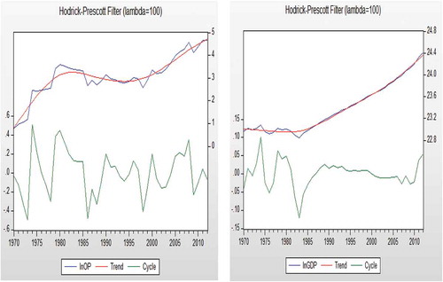
The outcome of prices of crude oil fluctuations on the growth of an economy is transmitted through both supply and demand channels (Jiménez-Rodríguez & Sánchez, 2005). In Ghana, increases in the world price of crude oil are transmitted into the domestic economy through increases in the domestic prices of petroleum products in the country. As a major source of input for the productive sectors of the economy, such increases tend to have serious repercussions on the country’s economic growth. For example, the oil prices and GDP generally increased within the period under study in a fluctuating manner (See Figure 1a and 1b). This study therefore explores the effect a price of crude oil has on economic growth in Ghana.

Figure 1. (a) Plotted series of filtered oil prices from 1970 to 2012. (b) Plotted series of filtered real GDP from 1970 to 2012.

2. Relevant literature

2.1. Oil price and economic growth

There is extensive empirical literature with respect to oil prices and its relationship with GDP covering the last three decades. Darby (1982) and Hamilton (1983) were among the early studies and they conclude that recessions that occurred within particular economies were followed by a fast rise in prices of crude oil. Over the years, this notion has weakened as later empirical studies that use data that extends beyond the 1980s show oil prices having less influence on economic output. Since the seminal work of Hamilton (1983), oil prices have been found to Granger-cause economic output on the US economy. Jiménez-Rodríguez and Sánchez (2004) identified similar results for Japan, Germany, France, Canada, Norway and the United Kingdom. These studies all focused on short-term interactions with few studies having considered the long-term relationship between the two factors. Hooker (2002), in an analysis on the US economy, estimated a cointegrating relationship that exists between oil prices, unemployment and interest rates over a long period, while Lardic and Mignon (2006) showed evidence of cointegration between prices of oil and GDP in the United States in addition to other countries within Europe. Another part of the oil price–GDP literature considered the role of responses from irregular fluctuations in the price of oil arguing that the influence of oil prices on economic output depends on whether a symmetric or asymmetric model specification is applied. Symmetry in response to oil prices implies that the response of output to a fall in oil prices turns out to be a true reflection of the response of a rise in oil prices of the same magnitude, whereas asymmetry, as the name suggests, implies that the response of output to a rise in oil prices differs to that of a fall in oil price of the same magnitude. Both specifications have been widely applied in investigating the direction of causality between oil prices and economic output in a time-series context. However, due to numerous challenges, no study has applied the asymmetric specification in a panel context to the oil price and GDP relationship. A considerable body of economic literature has shown the effect of oil prices on the economy of the United States and other OECD countries; however, there have been relatively fewer empirical studies on the non-OECD countries, and what has been undertaken in this area generally analysed the relationship in a time-series context. Lescaroux and Mignon (2008) is the only study that analysed the oil price–GDP relationship using a panel approach. Recently, panel data analysis has been enhanced since the technique can take the heterogeneous country effect into account. Against this background, this chapter aims to add to the literature by employing both time-series and causality techniques to investigate the long-term association existing between prices of oil and economic growth. According to Jiménez-Rodríguez and Sánchez (2004), the consequence of oil price fluctuations should vary among oil exporting as well as oil importing nations. The implication of this is that a rise in the oil price ought to reflect as good news in the former and bad news in the latter. It is therefore a priori expected that an increase in oil price affects countries that export oil positively and negatively influences countries that import oil.

2.2. Causality relationship that exists between oil prices and economic output

The causality testing framework has been mainly based on the Granger causality concept. Most of the earlier studies assumed a symmetric specification and generally found causality running from oil prices to GDP. The asymmetric specification is mostly based on Mork’s (1989) oil price increase and decrease. Likewise, Hamilton’s (1996a) net oil price increase specifications significantly improved the model description of the oil price–economic output relationship, which were elaborated upon in the studies that followed. Hooker (1996a) identified the changes in the causality link concerning oil prices and GDP while searching for a statistically stable specification. The works of Hooker (1996b) and Hamilton (1996b) have contributed massively in creating a steady statistical relationship between changes in price of oil and GDP. Generally, the model of transmission channels, together with interactions of the oil price–GDP association, has improved the comprehension of oil price influence on macroeconomic aggregates such as GDP. The first to report a weak statistical association concerning prices of oil and GDP was Hamilton (1983). According to Hamilton’s (1983) change in log of nominal oil prices has permitted a symmetric effect. The foundation for the direction (positive and negative) of GDP receptiveness to the changes in oil price was established by Mork (1989). This was the first non-symmetric description of the oil price–GDP relationship using variables that are distinct variables for fluctuations in prices. The association concerning oil price and GDP description was strengthened during the middle of 1980.

Hooker (1996a, 1996b) demonstrated that neither of the two specifications discussed above maintained a steady oil price–GDP association further than the early 1980s. A response from Hamilton (1996a) with regard to the Net Oil Price Increase description in relation to variable soil price was specified as the change between the maximum percentage increase in the price of oil within the present time frame and the former four quarters. Hamilton (1996b) extended his unique Net Oil Price Increase to a 3-year peak from a year peak. According to Hamilton (1996b), this specification captures the most surprising element with regard to change in oil price as it removes the increase in price that only corrects current reductions (Hooker, 1996c)

According to Rotemberg and Woodford (1996), these specifications enhanced the t statistic regressions, but did not address the issue of a steady, long-run association concerning prices of oil and other macroeconomic variables in their entirety. They further argued that the concept of “how much effect” still attracts interest to those responsible for policy formulation. Rotemberg and Woodford (1996) estimate that “an increase of 0.1 in oil price is predicted to contract output by 0.25, within a period of five to six quarters in the future”. The description of a related cumulative model by Finn (2000) reveals that variations in oil price enhance a fast, concurrent decline in energy consumption and utilization of resources. Using bivariate and multivariate vector auto-regression (VAR) specifications, Hooker (1999) examined the steadiness of the association of oil price and GDP over the time frame of 1954–1995. He identified that there was a direct link between oil price and output before 1980 and it seems as though its operation was via other indirect channels after 1980. Backus and Crucini (2000), in a study of US economy, found that instability within the terms of trade has a significant relationship with the increase in oil price instability in comparison to the flip side of the occurrence being exchange rate variations. Bercement, Ceylan, and Dogan (2009) examined the effects of oil prices on the growth of output of certain MENA countries that are well-thought-out to be either exporters or importers of oil using the time-series technique. The implication of these results indicate that an increase in the prices of oil has a statistically significant direct impact on the output of Algeria, Iran, Iraq, Kuwait, Libya, Oman, Qatar, Syria and the UAE. However, oil prices do not appear to have a statistically significant impact on the output of Bahrain, Djibouti, Egypt, Israel, Jordan, Morocco and Tunisia.

A study on the effect of oil prices on real macroeconomic activity by Aliyu (2009) in Nigeria employed both linear and non-linear description. The results of the study indicated both linear and non-linear impacts of oil price fluctuation on real GDP. Specifically, the article found that a non-symmetrical rise in oil price would have a greater effect on the growth of real GDP than the effect of non-symmetric decline in the price of oil on real GDP.

2.3. Crude oil price and the Ghanaian economy

Ghana’s macroeconomic performance has been associated with high and low points over the years. The period between 1973 and 1983 can be described as the dark years of the Ghanaian economy. During this period, the country experienced a downward spiral in economic growth, high rates of inflation, shortage of goods and services among others. Industrial output fell by 12.5%, budget deficit increased by 44.94%, total money supply climbed to over 500% cumulatively with inflation rate reaching 117% by 1977 (Fosu & Aryeetey, 2008; Hutchful, 2002). This period, as indicated earlier, coincided with the first two oil price shocks experienced by the world economy, as well as periods of political instability and economic mismanagement in Ghana.

Huge budget deficits in the past have been attributed to the provision of fuel subsidies by the government and this tends to have a negative effect on the Ghanaian economy. Periods of poor economic growth in the country was usually followed by a rise in crude oil price and huge fiscal deficits in the economy. Ocran (2007) maintains that a major cause of the huge fiscal deficits can be attributed to failure of the government to adjust the domestic price of petroleum products to reflect the rise in the world price of crude oil.

Similarly, a report by the Centre for Policy Analysis (2003) indicated that the public expenditure and currency crises of 2000, which continued into 2001 and 2002, was as a result of the continual rise in the international price of crude oil and the failure of government to pass it on to the consumer. Thus, the decision by the government to absorb increases in crude oil prices through subsidies rather than allowing for automatic price adjustments meant that the government expenditure exceeded its targets in those years. The cost of crude oil subsidies rose to about 2% of GDP by 2002. In January 2003, the government introduced a pricing formula that linked domestic prices to world prices to reduce the burden on the government in terms of subsidies. However, for political expediency, the automatic adjustment was deserted and further increases in the world price of crude oil were not conveyed to consumers but rather absorbed by the government through its expenditure. Despite high world oil prices that rose above $50.00 in 2004, the government maintained the low price and ended up subsidizing crude oil products to the tune of $200 million, representing 2.5% of GDP (Ocran, 2007). The government spends an average of $432 million annually on the subsidization of petroleum products in the country. Utility and fuel subsidies cost the government an amount of GH¢809.0 million in 2012, with an additional amount of GH¢955.8 million that was due to be paid in 2013 (Ministry of Finance and Economic Planning, 2013).

It is important to mention that the alternative of increasing the subsidy, even though popular politically, may perhaps have confrontational impact on the growth prospects of the economy. Large subsidies on domestic petroleum price may prevent government from spending on sectors of higher productivity or may lead to non-sustainable deficits of a budget. A rise in a subvention is always arising in public expenditure. In response to this increase in public expenditure, taxes must be raised, or certain public expenditure cut to prevent a rise in budget deficit due to an imbalance created within the actual trend.

There are three ways by which a government in developing countries can finance their expenditure: to print additional currency, to issue public debt or borrow from domestic financial institutions and through foreign borrowing. The Government of Ghana has, in the past, financed subsidies through finances borrowed from the domestic financial market or through the printing of money. Borrowing from the domestic financial market may result in the crowding out of private investment and may adversely affect growth of the economy. Similarly, the printing of additional currency may increase inflationary pressures on the economy. When a central bank does not monetize the deficit, modifications in the private sector to higher deficit policies may very well lead to inflation as is argued by Akçay, Alper, and Özmucur (2002). The predicament of an oil price surge for central banks is that it is often challenging from a stabilization policy viewpoint, in the sense that higher oil prices not only push up inflation (thus calling for a rise in interest rates) but also dampen growth (necessitating rates to be lower than otherwise) (Bank of Ghana, 2004).

3. Methodology

The study made use of secondary data. All the data series were collected from the World Development Indicators provided by the World Bank, except oil prices that were collected from the International Financial Statistics database provided by the International Monetary Fund. The data span from 1970 to 2012. The model employed is a simple relationship between oil prices and economic growth. The model is algebraically expressed as:

(1) $lnGD{P}_t={\beta }_0+{\beta }_{1}lnO{P}_t+{\epsilon }_t$(1)

where $lnGDP$ is the current rate of output which is used as a proxy for economic growth, $O{P}_t$ is the current rate of oil price, ${\epsilon }_t$ is a stochastic error term assumed to have a constant variance and a zero mean, ${\beta }_0$ is a constant term or the intercept of the economic growth–oil price nexus, and ${\beta }_1$ is the coefficient of oil price that is expected to be either positive or negative depending on whether the country is a net exporter or exporter of crude oil. It is therefore a priori expected that an increase in oil price will have a positive effect on the net oil exporting countries and a negative effect on the net oil importing countries. In the case of Ghana as a net importer of oil, and using the time frame of the data employed, economic theory postulates that an increase in oil prices would lead to an increase in the general price level and consequently slow economic activities and economic growth.

The data were analysed using descriptive statistics, Augmented Dicky-Fuller (ADF) test, Granger causality test and Johansen’s (1988) cointegration approach. The ADF test was used to test the unit root—that is, the level of stationarity in the time-series data. Non-stationary time series data when used in regression would lead to inconsistent and efficient parameter estimate. Hence, there is the need to examine the level of stationarity and if the data are non-stationary, it is important to address the problem before using it for regression analysis.

Therefore the ADF test was used to examine the existence or otherwise of unit root in the data set. The ADF test was employed because it is simple and is a more expedient procedure that can be used to examine the time-series data. However, in an ADF test, there is loss of observation; hence, the Phillips–Perron (PP) (1988) unit root test is applied to augment the ADF because of its use of non-parametric methods to adjust for serial correlation and endogeneity of regressors, thereby preventing the loss of observations implied by the ADF test. It also allows for the possibility of heteroskedastic error terms (Hamilton, 2009).The approach likewise controls for higher order correlation by adding lagged difference terms of the dependent variables. The model is specified as follows:

(2) $\mathrm{\Delta }{y}_t=\alpha +\delta y_{t-1}+\sum _p^{t=1}{\gamma }_i\mathrm{\Delta }{y}_{t-1}+{\epsilon }_t,$(2)

where $y_t$ represents the data set from individual variables—that is, oil prices and GDP. $\alpha$ is the intercept term, $\delta$ is the coefficient for the unit root test, while $\gamma$ is the parameter of the augmented lagged difference.

From the above test (regression) p-values are used to reject or not to reject the hypothesis and the decision rule is that if $\delta =0$, then it means the test has failed to reject the null hypothesis implying that the data are non-stationary; hence, there is a presence of a unit root. Alternatively, if $\delta \ne 0$ that if the test fails to reject the alternative hypothesis, then it means unit root does not exist in the data set; hence, the data are stationary.

After having verified the presences of the unit root in the data, the Johansen cointegration test procedure is applied to establish the long-run relationship between economic growth and oil prices. Johansen’s (1988) cointegration technique takes its starting point in the VAR of order p given by;

(3) $y_t=\mu +A_1{y}_{t-1}+..\dots ..\dots \dots .+A_p{y}_{t-p}+{\epsilon }_t$(3)

where $y_t$ is an $nx1$ vector of variables that are integrated of order one.

Equation (3) can be rewritten as:

(4) $\mathrm{\Delta }{y}_t=\mu +\mathrm{\Pi }{y}_{t-1}+\sum _{p-1}^{i=1}{\mathrm{\Gamma }}_{\mathrm{\Delta }i}{y}_{t-i}+{\epsilon }_t,$(4)

where $\mathrm{\Pi }=\sum _{i=1}^p{A}_i-I$ and $\mathrm{\Gamma }=-\sum _{j=i+1}^p{A}_j$.

Johansen proposed two different likelihood ratio tests—the trace test and maximum likelihood test, shown in the following equations, respectively. Since Johansen’s test can be used to test multivariate cointegration, $y_t$here represents all the variables in the equation:

(5) $J_{trace}=-T\sum _{i=r+1}^n\mathrm{l}\mathrm{n}(1-{\hat{\lambda }}_i)$(5)

(6) $J_{max}=-Tln\left(1-{\hat{\lambda }}_{r+1}\right)$(6)

Here, T is the sample size and ${\hat{\lambda }}_i$ is the i th largest canonical correlation. The trace test tests the null hypothesis of r cointegrating vectors against the alternative hypothesis of no cointegrating vectors. The maximum eigenvalue test, on the other hand, tests the null hypothesis of r cointegrating vectors against the alternative hypothesis of r + 1 cointegrating vectors. Since the critical values used for the maximum eigenvalue and trace test statistics are based on a pure unit root assumption, they will no longer be correct when the variables in the system are near unit root processes.

As a robust check, the estimates were evaluated using the long-run multipliers by semi-parametric fully modified least squares (FMOLS) and dynamic fully modified ordinary least squares (DOLS) estimators following Philips and Hansen (1990) and Stock and Watson (1993), respectively. Furthermore, the Granger causality test was used to examine the causal link between the oil prices and GDP in Ghana. The test was used to examine if there is a unidirectional or bidirectional relationship between the variables as a result of independence between the variables under consideration. Granger (1969) defined lead and lag relations based on the role of predictability in which he used VAR to test or find causal relationship between the factors. This test is known as Granger causality test. The equation to test the causal relation between the two series, $OP$ (oil prices) and $GDP$(GDP), can be specified as follows:

(7) $lnGD{P}_t={\alpha }_0+\sum _{i=1}^l{\alpha }_{1i}lnGD{P}_{t-i}+\sum _{i=1}^l{\alpha }_{2i}lnO{P}_{t-i}+{\epsilon }_{1t}$(7)

(8) $lnO{P}_t={\beta }_0+\sum _{i=1}^l{\beta }_{1i}lnGD{P}_{t-i}+\sum _{i=1}^l{\beta }_{2i}lnO{P}_{t-i}+{\epsilon }_{2t}$(8)

where ${\alpha }_0$ and ${\beta }_0$ are the intercept terms, ${\alpha }_{1i}$ and ${\beta }_{1i}$ are the coefficients of the lagged dependent variables, ${\alpha }_{2i}$and ${\beta }_{2i}$ are parameters of the independent variables, while ${\epsilon }_{1t}$ and ${\epsilon }_{2t}$ are the error terms and $i$ to $k$ are the number of lags. The optimum lag length is selected based on the Akaike information criteria (AIC). The above equation tests the following hypothesis:

Null hypothesis [H0: no-Granger causality] i.e., $\sum _{i=1}^k{\alpha }_{2i}=0$ and $\sum _{i=1}^k{\beta }_{2i}=0$, respectively.

Alternative hypothesis [H1: Granger causality exists] i.e., $\sum _{i=1}^k{\alpha }_{2i}\ne 0$ and $\sum _{i=1}^k{\beta }_{2i}\ne 0$, respectively.

Thus, if the null hypothesis is rejected, then it means the coefficient is statistically equal to zero simultaneously. This means that the past and present values of oil prices provide no important information to predict future value of oil prices.

The following are used to test the relationship between the variables or how one variable causes the other variable.

${\alpha }_{2i}\ne 0$ and ${\alpha }_{1i}=0$: It means $OP$ leads $GDP$ or $GDP$ lags $OP$.

${\beta }_{1i}\ne 0$ and ${\beta }_{2i}=0$: It means $GDP$ leads $OP$ or $OP$ lags $GDP$.

${\alpha }_{2i}=0$ and ${\beta }_{1i}=0$: It means that both of the variables are independent.

${\alpha }_{2i}\ne 0$ and ${\beta }_{1i}\ne 0$: It means that both of the variables interactive with each other and have a feedback relationship.

4. Results and discussions

Results in Table 1 show the descriptive statistics of the variables. The results show that the mean values of real GDP and oil prices have remained positive throughout the period studied. However, oil prices experienced a high volatility rate as shown in the standard deviation of 26.464 against 4.769 for real GDP growth. The relative high volatility in oil prices is also depicted in the cyclical components of filtered data in Figure 1a.

Table 1. Descriptive statistics of variables

Indicators	1970–1979	1980 −1989	1990–1999	2000–2009	2010–2012	Mean	St. dev	Max	Min
Real GDP growth	1.446	1.993	4.265	5.364	10.413	3.766	4.769	14.046	−12.432
Per capita GDP growth	−0.842	−1.013	1.580	2.686	7.732	1.100	4.689	11.278	−14.455
Oil price	10.069	25.172	18.202	49.173	96.016	30.563	26.464	105.008	2.180

Figure 1b shows that series of log of real GDP shows an increasing trend—that is, the series of log of real GDP drifts upwards. The series of nominal oil price levels (Figure 1a) likewise shows an upward movement; hence, it justifies the inclusion of trend in the analysis.

5. Result of the unit root test

Prior to estimating the effect of real oil prices on economic growth, the order of integration of the data was examined using the ADF and PP unit root test. The variables were tested at the level and after first differencing to examine the order of integration of each variable. The results of the unit root test are shown in Tables 2 and 3.

Table 2. ADF and PP unit root test without a trend

ADF unit root test without a trend			PP unit root test without a trend
Variable	Test statistic at level	Test statistic at 1st difference	Test statistic at level	Test statistic at 1st difference
lnGDP	3.603	−4.143**	3.525	−4.142**
lnOP	−2.55	−6.029***	−2.567	−6.026***

Note: ** and *** are significance levels at 10%, 5% and 1%, respectively.

Table 3. ADF and PP unit root test with a trend

ADF unit root test without a trend			PP unit root test without a trend
Variable	Test statistic at level	Test statistic at 1st difference	Test statistic at level	Test statistic at 1st difference
lnGDP	3.603	−4.143**	3.525	−4.142**
lnOP	−2.55	−6.029***	−2.567	−6.026***

Note: ** and *** are significance levels at 10%, 5% and 1%, respectively.

Table 2 shows the results of the unit root test without a trend in the series of real GDP and nominal oil price levels. The table depicts that both log of real GDP and the nominal oil price level are non-stationary at the level at conventional levels of significance. However, stationarity of the variables were achieved after first differencing. Thus, both real GDP and the oil price levels are cointegrated of order one, and therefore justify the use of the Johansen cointegration techniques solely designed for I(1). Table 2 shows that log of real GDP was stationary at 5% significance level, whereas log of nominal oil prices achieved stationarity at 10% significance levels after first differencing.

Table 3 furthermore shows the results of the unit root test in the data series of log of real GDP and log of nominal price levels. The results clearly depict a similar result as to when trend was removed from the test procedure. The results show that all the variables were non-stationary at the level at conventional levels of significance. However, after first differencing all the variables, log of real GDP was stationary at 5% significance levels, whereas the nominal oil price rate achieved stationarity at 10% conventional level of significance. This implies that both log of real GDP used as a proxy for economic growth and log of oil price level are integrated of order I(1) and therefore justifies the use of the Johansen technique of cointegration designed solely for$I\left(1\right)$.

6. Selection of lag order

Before proceeding with the estimation of the model with Johansen cointegration method, a test of the selection criterion of maximum lag for cointegration was conducted to choose a criterion and the maximum lag to be used. Since the lag length is not derived from theory it needed to be determined by comparing different specifications. As a benchmark, the various information criterion was examined. In Table 4, the Schwarz information criterion (SBIC) and the Hannan-Quinn information criterion (HQC) indicated a maximum lag of (1). However, the Akaike information criterion (AIC) and the Final Prediction Error (FPE) indicated a maximum lag length of (3). Although the AIC is not a consistent order-selection criterion and additionally tends to overestimate the maximum lag length, it is still used since it better suits the model and the data employed (Brockwell & Davis, 2002). The result of the lag-order selection is shown in Table 4.

Table 4. Selection-order criteria

lag	LL	LR	df	p	FPE	AIC	HQIC	SBIC
0	−47.0263				0.042359	2.51417	2.54478	2.59948
1	64.668	223.39	4	0.000	0.000169	−3.00861	−2.91679*	−2.75268*
2	69.2346	9.1332	4	0.058	0.000165	−3.03767	−2.88463	−2.50406-
3	74.4741	10.479*	4	0.033	0.000155*	−3.10124*	−2.88698	−2.61112
4	76.895	4.8417	4	0.304	0.00017	−3.02026	−2.74478	−2.25246

Note: * represents 10% significance level.

LL and LR represent log likelihood and likelihood ratio respectively.

7. Result of the cointegration test

Johansen’s maximum likelihood method of cointegration is employed in establishing the effect of oil price change on economic growth. The result is shown in Table 5.The result above shows that a long-run relationship exists between oil prices and economic growth. Using the trace statistics indicated the presence of two cointegrating equations at 5% significance level, whereas the maximum likelihood statistics also indicated the presence of two cointegrating equations at 5% significance level. In other words, both the trace statistics and the maximum likelihood statistics indicated a long-run relationship between oil price levels and economic growth.

Table 5. Johansen cointegration test

Result from Johansen cointegration test
Null hypothesis	${\mathit{J}}_{\mathit{t}\mathit{r}\mathit{a}\mathit{c}\mathit{e}}$	${\mathit{J}}_{\mathit{m}\mathit{a}\mathit{x}}$	Conclusion
r = 0	36.18263	22.81848	Evidence of cointegration
	(0.0018)**	(0.0152)**
r = 1	13.36415	13.36415	Evidence of cointegration
	(0.036)**	(0.036)**

Note: p-values are in parenthesis and ** represents 5% level of significance.

Table 5 shows the long-run estimate of the effect of oil prices on economic growth. From Table 5, the adjusted coefficient of determination (${\bar{\mathrm{R}}}^2$), used to measure the goodness-of-fit of the estimated model, is high enough to indicate that the model is reasonably accurate in making a prediction. It suggests that, approximately, between 87% and 95% of the variations in economic growth is accounted for by changes in oil prices. The high (${\bar{\mathrm{R}}}^2$) shows that the problem of multicollinearity is minimized. The variables were logged to bring all of them into the same unit to minimize the problem of autocorrelation and heteroskedasticity. Table 6 presents the results of the estimated parameters of the effect of oil price change on economic growth.

It was expected that the coefficient on the oil prices would be negative; that is, a high rate of oil prices feeds into the high general price levels, which consequently leads to slow economic activities in the long run. Consequently, this was the result achieved as the results depict an inverse relationship between oil price and economic growth. The results are aligned with the empirical work of Rodriguez and Sanchez (2004), who concluded that the consequence of oil price fluctuations should be different in oil exporting and oil importing countries as an increase should be considered good news in the former and bad news in the latter. It is therefore a priori expected that an increase in oil price will have a positive effect on the net oil exporting countries and a negative effect on the net oil importing countries. In line with this study, Ghana has been a net importer of oil and it was expected that increasing oil prices would have a daunting effect on the Ghanaian economy, and therefore justifies the inverse oil price change and economic growth nexus results obtained.

The results show that oil price changes have no significant effect on economic growth at 5% significance level. In other words, changing oil prices does not account for changes in economic growth when log of GDP is used as a proxy. This fits into neoclassical economic theory, which teaches that changes in real variables are independent of changes in nominal variables. However, Bercement et al. (2009) examined how oil prices affect the output growth of selected MENA countries that are considered either net exporters or net importers of oil using the time-series technique and found that an oil price increase had a statistically significant and positive impact on the output of Algeria, Iran, Iraq, Kuwait, Libya, Oman, Qatar, Syria and the UAE. The differences in this analysis and that of Bercement et al. (2009) could be accounted for by the fact that, whereas Ghana has been a net importer of crude oil over the time frame, Algeria, Iran, Iraq, Kuwait, Libya, Oman, Qatar, Syria and the UAE are net exporters of crude oil. Aliyu (2009) likewise analysed the effect of oil prices on real macroeconomic activity in Nigeria employing both linear and non-linear specifications. The article finds evidence of both linear and non-linear impacts of oil price shocks on real GDP. It is also worth mentioning that Nigeria is a net exporter of crude oil; hence, the result supports that of Bercement et al. (2009). Again, Rotemberg and Woodford (1996) estimate that “a 10% increase in the price of oil is predicted to contract output by 2.5%, 5 or 6 quarters later”. Finn’s (2000) specification of a similar aggregate model reveals that an oil price shock causes sharp, simultaneous decreases in energy use and capital utilization. In congruent with this study, the result supports the findings of Bercement et al. (2009) who concluded that oil prices do not appear to have a statistically significant impact on the output of net crude oil importing countries like Bahrain, Djibouti, Egypt, Morocco and Tunisia.

The results from our robust check (FMOLS and DOLS) depict an inverse relationship as shown by the Johansen method, therefore making the result more parsimonious. The trend is significant in the model at 5% significance level in all models.

8. Granger causality test

Two hypotheses were tested on Granger causality, with economic growth which log of GDP is used as a proxy for economic growth and the log of oil prices. Two different models were tested: first Granger causality was tested to determine if oil prices could be used to accurately predict fluctuations in the economic growth (from Hypothesis 1, Table 7; and the second hypothesis was to test if Granger causality existed in the reverse direction (i.e., if economic growth (output growth) was Granger-causal to oil prices) (Hypothesis 2, Table 7). The results of the first hypothesis depict a causal relationship between oil prices and economic growth; hence, the null hypothesis is rejected. Thus, log of oil prices Granger cause log of GDP; in other words, changes in oil prices could be used to predict changes in economic growth and this supports the econometric specification of the model employed and the cointegrating relationship obtained from the Johansen cointegration technique to estimate the effect of oil price change on economic growth. This direction of causation is in line with the conclusions of the seminal work of Hamilton (1983) that oil prices Granger cause economic output on the US economy and another 54 similar results were found for Japan, Germany, France, Canada, Norway and the United Kingdom by Jimenez-Rodriguez and Sanchez (2004).The reverse causality shows that log of GDP does not Granger cause oil price change. In this scenario, we failed to reject the null hypothesis as the p-value is greater than 0.05 meaning log of GDP has no significant influence on oil price changes in the long run.

Table 6. Estimated long-run relationship between economic growth and oil prices

Variable	Johansen	FMOLS	DOLS
$lnOP$	−0.134674	−0.042139	−0.019406
	(0.05408)	(0.4320)	(0.6899)
$Trend$	0.033255	0.039237	0.037842
	(0.00468)**	(0.0000)**	(0.0000)**
$C$	-	8.577781	8.465913
	-	(0.0000)**	(0.0000)**
${\bar{R}}^2$	-	0.87	0.95
$N$	39	42	40

Note: p-value are in parenthesis and ** represents 5% level of significance.

Table 7. Granger causality between oil price and economic growth

Hypothesis	F-statistic	p-Value	Decision
$lnOP$ does not Granger cause $lnGDP$	$5.53$	$0.0035$	Reject null hypothesis
$lnGDP$ does not Granger cause $lnOP$	$2.71$	$0.0609$	Do not reject null hypothesis

9. Conclusion and policy implications

Employing the Johansen approach to cointegration, the results showed a negative relationship between oil prices and economic growth. This implies that, as oil prices go up, economic growth (where log of real GDP is used as a proxy) falls. This supports the theoretical assumption that oil price changes lead to an increase in the general price level and consequently slows economic activities and economic growth.

The next objective was to find the causal linkage between oil price change and economic growth. Applying the Granger causality test showed that oil price change Granger causes economic growth, but economic growth does not Granger cause oil price changes. In other words, there is a unidirectional causation from oil price change to economic growth.

Given the results above, economic policies that seek to influence economic growth (real GDP) through changing oil prices would seem ineffective due to the statistical insignificance of the effect of oil price change on real GDP. It is therefore recommended that macroeconomic policies that seek to influence economic growth should be pursued independently of changing oil prices.

Additional information

Funding

The authors received no direct funding for this research.

Notes on contributors

Dadson Awunyo-Vitor

Dadson Awunyo-Vitor is a Senior Lecturer at the Department of Agricultural Economics, Agribusiness and Extension, KNUST in Ghana. One of his recent publications is: Adusei, C. and Awunyo-Vitor D (2017). Profitability determinants of abattoir business in an emerging economy, International Journal of Accounting and Finance, 7(4), 335–351. This paper is culled from the dissertation Dadson supervised.

Solomon Samanhyia

Solomon Samanhyia is the thesis coordinator at the Ghana Technology University College, Kumasi Campus. He is currently undertaking an advanced Master’s Program in Development Evaluation and Management at University of Antwerpen, Belgium.

Elijah Addo Bonney

Elijah Addo Bonney works with Ministry of Health in Ghana and completed his MBA in Finance from the Coventry University, UK. This paper is culled from his MBA dissertation.

References

- Akçay, O. C., Alper, C. E., & Özmucur, S. (2002). Budget deficit, inflation and debt sustainability: Evidence from Turkey (1970–2000). In A. Kibritcioglu, L. Rittenberg, & F. Selcuk (Eds.), Inflation and disinflation in Turkey (pp. 77–96). London: U.K. Ashgate.
- Aliyu, S. U. R. (2009). Oil price shocks and the macro-economy of Nigeria: A non-linear approach. MPRA Working Paper, Bayero University, Kano.
- Amano, R., & Van Norden, S. (1998). Oil prices and the rise and fall of the US real exchange rate. Journal of International Money and Finance, 17, 299–316. doi:10.1016/S0261-5606(98)00004-7
- Andrews, D. (1993). Tests for parameter instability and structural change with unknown change point. Econometrica, 61, 821–856. doi:10.2307/2951764
- Andrews, D., & Ploeberger, W. (1994). Optimal tests when a nuisance parameter is present only under the alternative. Econometrica, 62, 1383–1414.
- Armah, B. (2003). Economic analysis of the energy sector.. Accra: Ghana Energy Commission.
- Aryeetey, E., & Harrigan, J. (2000). Macroeconomic & sectoral developments since 1970. In E. Aryeetey, J. Harrigan, & M. Nissanke (Eds.), Economic reforms in Ghana. The miracle and the mirage. Oxford: James Currey.
- Backus, D., & Crucini, M. (2000). Oil prices and the terms of trade. Journal of International Economics, 50, 185–213. doi:10.1016/S0022-1996(98)00064-6
- Bank of Ghana. (2004). 2004 Annual report of Bank of Ghana, Accra.
- Bercement, H. B., Ceylan, N., & Dogan, N. (2009). The impact of oil price shock on the economic growth of MENA countries. The Energy Journal, 31(1), 149–176
- British Petrochemical. (2012). Energy outlook 2030. Retrived from, www.bp.com/sectiongenericarticle800.do?categoryId=9037134&contentId=7068677
- Brockwell, P. J., & Davis, R. A. (2002). Introduction to time series and forecasting. USA: Springer-Verlag New York.
- Centre for Policy Analysis. (2003). The state of the Ghanaian economy 2002–2003. Accra: Author.
- Centre for Study of Africa Economies (CSAE) (2014). Crude oil price and economic growth: The case of Ghana. Conference paper.
- Darby, M. R. (1982). The price of oil and world inflation and recession. American Economic Review, 72, 738–751.
- Finn, M. G. (2000). Perfect competition and the effect of energy price increase on economic activity. Journal of Money, Credit and Banking, 32, 400–416. doi:10.2307/2601172
- Fosu, A. K., & Aryeetey, E. (2008). Ghana’s post independence economic growth, 1960–2000. In E. Aryeetey & R. Kanbur (Eds.), The economy of Ghana: Analytical perspectives on stability, growth & poverty (pp. 36–77). Accra: Woeli Publishing Services.
- Granger, W. J. (1969). Investigating causal relations by econometric models and cross spectral methods. Econometrical, 36, 424–438. doi:10.2307/1912791
- Hamilton, J. D. (1983). Oil and the macro economy since World War II. Journal of Political Economy, 91, 228–248. doi:10.1086/261140
- Hamilton, J. D. (1996a). This is what happened to the oil price-macro economy relationship. Journal of Monetary Economics, 38, 215–220. doi:10.1016/S0304-3932(96)01282-2
- Hamilton, J. D. (1996b). Analysis of the transmission of oil price shocks through the macro economy Paper presented at the DOE conference. International Energy Security, Washington, D.C.
- Hamilton, J. D. (2009). Causes and consequences of the oil shock of 2007–08. NBER Working Paper No. 15002.
- Hooker, M. A. (1996a). What happened to the oil price-macroeconomy relationship? Journalof MonetaryEconomics, 38, 195–213.
- Hooker, M. A. (1996b). This is what happened to the oil price-macroeconomy relationship: Reply. Journal of Monetary Economics, 38, 221–222. doi:10.1016/S0304-3932(96)01283-4
- Hooker, M. A. (1996c). Exploring the robustness of the oil price-macroeconomy relationship: Empirical specifications and the role of monetary policy., Paper presented at the DOE conference. International Energy Security: Economic Vulnerability to Oil Price Shocks, Washington, D.C., October 1996.
- Hooker, M. A. (1999). Oil and the macroeconomy revisited. Washington, D.C.: Mimeo Federal Reserve Board.
- Hooker, M. A. (2002). Are oil shocks inflationary? Asymmetric and non-linear specifications versus changes in regime. Journal of Money, Credit and Banking,34, (2), 540–561. doi:10.1353/mcb.2002.0041
- Hutchful, E. 2002. Ghana’s adjustment experience, the paradox of reform. United Nations Research Institute for Social Development (UNRISD). London: James Currey.
- International Energy Agency. (2012). 2011 key world energy statistics. International Energy Agency. Retrieved November 2, 2012, from www.iea.org
- Jiménez-Rodríguez, R., & Sánchez, M. (2004). Oil price shock and real GDP growth: Empirical evidence for some OECD countries. European Central Bank Working Paper No. 362.
- Jiménez-Rodríguez, R., & Sánchez, M. (2005). Oil price shocks and real GDP growth; empirical evidence for some. Applied Economics, 37, 201–228. doi:10.1080/0003684042000281561
- Johansen, S. (1988). Statistical analysis of cointegration vectors. Journal of Economic Dynamics and Control, 12(2–3), 231–254. doi:10.1016/0165-1889(88)90041-3
- Killick, T. (2010). Development economics in action: A study of economics policies in Ghana. New York: Rutledge.
- Lardic, S., & Mignon, V. (2006). The impact of oil prices on GDP in European countries: An empirical investigation based on asymmetric cointegration. Energy Policy, 34, 3910–3915. doi:10.1016/j.enpol.2005.09.019
- Lescaroux, S., & Mignon, V. (2008). On the influence of oil prices and other macroeconomic and financial variables. CEPII, Working Paper No 2008.05.
- Mork, K. A. (1989). Oil and the macro economy when price go up and down: An extension of Hamilton’s results. Journal of Political Economy, 97, 740–744. doi:10.1086/261625
- Ocran, M. K. (2007). A modelling of Ghana’s inflation experience: 1960–2003. AERC Research Paper 169.
- Philips, P. C. B., & Hansen, B. E. (1990). Statistical inference in instrumental variable regression with I(1) processes. Review of Economic Studies, 57, 99–125. doi:10.2307/2297545
- Rotemberg, J., & Woodford, M. (1996). Imperfect competition and the effect of energy price increases on economic activity. Journal of Money, Credit and Banking, 28, 549–577. doi:10.2307/2078071
- Stock, J. K., & Watson, M. (1993). A simple estimator of cointegrating vectors in higher order integrated systems. Econometrica, 61, 783–820. doi:10.2307/2951763