
 ?Mathematical formulae have been encoded as MathML and are displayed in this HTML version using MathJax in order to improve their display. Uncheck the box to turn MathJax off. This feature requires Javascript. Click on a formula to zoom.
Abstract
To date the existence of jumps in different sectors of the financial market is certain and the commodity market is no exception. While there are various models in literature on how to capture these jumps, we restrict ourselves to using subordinated Brownian motion by an α-stable process, α ∈ (0,1), as the source of randomness in the spot price model to determine commodity future prices, a concept which is not new either. However, the key feature in our pricing approach is the new simple technique derived from our novel theory for subordinated affine structure models. Different from existing filtering methods for models with latent variables, we show that the commodity future price under a one factor model with a subordinated random source driver, can be expressed in terms of the subordinator which can then be reduced to the latent regression models commonly used in population dynamics with their parameters easily estimated using the expectation maximisation method. In our case, the underlying joint probability distribution is a combination of the Gaussian and stable densities.
PUBLIC INTEREST STATEMENT
This paper is entitled Subordinated Affine Structure Models for Commodity Futures Prices. The aim is to provide a mathematical background on a special family of processes that could capture unusual patterns such as extreme events in the commodities market. Such events could range from wild fires on farms to Tsunamis and as a result the commodities spot prices would be affected significantly. This realisation provides the motivation of the study in this paper. As a risk mitigation process, it is undeniable that investors in the commodities market would be interested in how this kind of risk could be captured in the future pricing model and more so, how the model would be calibrated to historical data. The current paper seeks to answer these questions and establishing a novel approach on pricing commodities futures.
1. Literature
A large volume of literature on commodities market has been published since the invention of the continuous benchmark model of Black and Scholes (Citation1973) for pricing options and corporate liabilities. Among the many models developed, the widely used and referenced study on commodities is the work by Schwartz (Citation1997). From the latter, numerous models have been developed as a result of the growing commodities market in terms of volumes traded and complexities of their contracts over the years. We give an account of the various literatures relevant to this research in Table .
Table 1. Various commodity jump models
The current research builds on findings from Kyriakou, Nomikos, Pouliasis, and Papapostolou (Citation2016) by extending the results to subordinated Brownian motion.
A selection of key commodity jump models that have developed overtime.
2. Introduction
Commodities exhibit distinctive features that a good model ought to capture. For instance to estimate the commodities market as closely as possible, one has to factor in jumps in the underlying spot price. However, models designed with a jump component are non-trivial. In this research, we derive a relatively easy estimation method for commodities prices using subordination as a proxy for introducing jumps. Other features include mean-reversion, contango, backwardation and seasonality. Commodities also experience extreme volatility and price spikes resulting in heavy-tailed distribution of the returns. Commodity markets are unique compared with other markets such as equity, bond, currency or interest rate markets in the sense that most commodities are real physical assets that are produced, transported, stored and consumed. They are not assets valued on long-lived companies like in equity markets.
As indicated in Fama and French (Citation1988), commodity pricing can be approached from two perspectives, the theory of storage which explains why high supplies and inventories running at minimum would result into contango, low futures and spot price volatilities, and in turn futures premiums being equivalent to full storage costs. On the other hand, why low supplies and enhanced production inventory levels yield to backwardation, a rise in volatilities of the spot and the nearby future prices. Another feature explained by this theory is the periodically continuously compounded convenience yield (usually denoted by ) on inventory which is the benefit of holding a physical commodity as opposed to having a future contract of its delivery at some future time and second, the cost of storage. The future price motivated by the theory of storage is given by
where accounts for the storage costs,
is the periodically continuously compounded interest rate,
is the current spot price and
is the maturity date of the future contract.
The second perspective is the theory of expected risk premium discussed in Keynes (Citation1930) and Hicks (Citation1939). It asserts that the future prices are given by the discounted (by the risk premium) expected future spot price:
where is the risk premium and
,
is the filtration up to time
.
A number of models based on the latter approach have been developed over the years to mimic the market as closely as possible for various commodities. This includes Schwartz’s common continuous stochastic factor models Schwartz (Citation1997), Schwartz and Smith (Citation2000) and the jump models of Kyriakou et al. (Citation2016).
The motivation and contribution of this paper are based on the existing erratic features in electricity and energy markets, where jumps are evident, resulting in skewed distributions of the spot prices. We consider a subordinated Brownian motion by an -stable process,
, as the source of randomness in the underlying asset to model commodity future prices. The stunning feature in our pricing approach is the new simple technique derived from our novel approach for subordinated affine structure models.
We show that the affine property is attainable and applicable to generalised commodity spot models, and as illustration, we consider a stochastic differential equation with subordinated Brownian motion as the source of randomness to derive the commodity future prices. It is argued in some existing literature that the likelihood function exists in integrated form for models with singular noise meanwhile for cases of partially observed processes, a filtering technique is required, see for instance Date and Ponomareva (Citation2010) and Yang, Lin, Luk, and Nahar (Citation2014). However, the work presented in this paper provides a new approach of pricing commodity futures for models with latent variables using the maximum expectation maximisation. We show that the commodity future price under a one-factor model with a subordinated random source driver can be expressed in terms of the subordinator, which can then be reduced to the latent regression models commonly used in population dynamics with their parameters estimated easily using the expectation maximisation method. In our case, the underlying joint probability distribution is a combination of Gaussian and stable densities.
The rest of the paper is organised as follows. The following Section 3 introduces some features of stable processes essential to this work. In Section 4, we review the concept of affine models and extend the idea of obtaining Laplace transforms of random processes to subordinated processes. In Section 5, we derive our pricing formulas for commodity futures using the results derived in Section 4. In Section 6, we discuss the numerical implementation of our one-factor commodity future models. Section 7 concludes.
3. Stable processes
The discussion in this section is mainly based on Kateregga et al. (Citation2017). A stable or -stable process,
, belongs to the general class of Lévy distributions. It has a limiting distribution with a definitive exponent parameter
that determines its shape. The following two definitions follow from Rachev (Citation2003).
Definition 3.1 Let be independent and identically distributed random variables and suppose a random variable
defined by
where “→” represents weak convergence in distribution, is a positive constant and
is real. Then,
is a stable process. The constants
and
need not to be finite.
Definition 3.1 allows the modelling of a number of natural phenomena beyond normality using stable distributions. The fact that and
do not necessarily need to be finite provides the generalised central limit theorem.
Definition 3.2 (Generalised Central Limit Theorem) Suppose , denotes a sequence of identically distributed independent random variables from some arbitrary distribution and let sequences
and
. Then, we define a sequence
of sums such that their distribution functions weakly converge to some limiting distribution. That is
The traditional central limit theorem assumes finite mean and finite variance
and defines the sequence of sums
Definition 3.3 Samoradnitsky and Taqqu (Citation1994) An -stable distribution is a four-parameter family of distributions denoted by
where
(1) is the characteristic exponent responsible for the tail of the distribution.
(2) is responsible for skewness.
(3) is the scale parameter (sometimes referred to as variance when
).
(4) is the location (sometimes referred to as mean).
Densities of -stable distributions do not have closed-form representations except the Gaussian (
), Cauchy (
) and Inverse Gaussian or Pearson (
) distributions.
The analysis of stable processes is usually through their characteristic functions and Laplace or Fourier transformation. Unlike their densities, their characteristic functions always exist. Literature on their integral representations and density functions is provided in Zolotarev (Citation1964), Citation1980, Zolotarev (Citation1986)). The distribution functions for the different values have been tabulated in Dumouchel (Citation1971), Fama and Roll (Citation1968) and Holt and Crow (Citation1973).
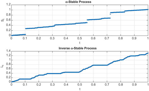
Definition 3.4 (Gajda and Wyłoman`Ska (Citation2012)) Let and
denote an α-stable process and its respective inverse. Then for
, we define the process
asFootnote1
and
are non-decreasing and cádlág with their graphical representations given in Figure .
Figure 1. The top graph shows a plot of a stable process and the bottom graph shows its inverse process
simulated using exponent parameter value,
, plotted against time on the horizontal.
3.1. Density and characteristic functions
Let denote a Lévy process. The characterisation of
is usually given by the Lévy–Khintchine formula.
Definition 3.5 (Lévy–Khintchine) Applebaum (Citation2004) Consider a Lévy process . There exists
and
such that the characteristic function of
is
where is the indicator function and
is a
-finite measure satisfying the constraint
Definition 3.6 (The Lévy-Itô Decomposition) Applebaum (Citation2004) If is a Lévy process, there exists
, a Brownian motion
with variance
and an independent Poisson random measure
on
such that, for each
,
where
To preserve the martingale property, the compound Poisson random measure is compensated as where
is a Lévy measure satisfying (11).
For process , we require
in (10) or
in (12) and the Lévy measure in (11) given by
The characteristic function of
is obtained using the domain of attraction of stable random variables (See Grigelionis, Kubilius, Paulauskas, Statulevicius, & Pragarauskas, Citation1999) and the Lévy–Khinchine representation formula (See Definition 3.5 or Applebaum (Citation2004) for a detailed explanation), i.e.
Using Fourier transformation, the density function of is given by
From Definition 3.4, it is easy to see the equivalence relation
It follows that where
denotes the probability density function of
. Consequently
According to Meerschaert and Straka (Citation2013), the density can also be given by
where is the density of a standard stable process with a Laplace transform
. This follows from the fact that
has the same distribution as
. As a result, the density of the inverse stable process
can be given in terms of the standard stable process by
Figure shows density graphs of for different exponent parameter values.
Figure 2. The graphs represent densities of an -stable process for different values of the exponent parameter,
. Observe the variation in the tail sizes and the skewness as the exponent parameter is varied.
![Figure 2. The graphs represent densities of an α-stable process for different values of the exponent parameter, α ∈(0,2]. Observe the variation in the tail sizes and the skewness as the exponent parameter is varied.](/cms/asset/c4141b2b-f629-46cc-a52a-d4ad0828d457/oaef_a_1512360_f0002_c.jpg)
3.2. Laplace transforms
Definition 3.7 Let be a subordinator. The Laplace transform of
is defined by
where is the Laplace exponent of
known as the Bernstein function represented by
where and
is the Lévy measure on
such that
The Laplace transform of the stable process is given by (see Meerschaert & Straka, Citation2013)
where . For
(alternatively
), the Laplace transform simplifies to that of a standard stable process:
The Laplace transform of the inverse stable process
is obtained from (18):
where the Laplace transform of is
and
for
or
. Since (25) does not have the general form for a Laplace transform of a Lévy process, then
is not a Lévy process.
3.3. Moment-generating function
There is a relationship between a moment-generating function of a random variable and its Laplace transform.
Lemma 3.8 Let and
denote the respective moment-generating function and Laplace transform of a random variable then
where
Proof 3.9 This relationship is verified in Miller (Citation1951).
As a consequence of Lemma 3.8 and the explicit Laplace transform given by (23), we can deduce the first and second moments of . That is
3.4. Subordination
Let denote subordinated Brownian motion where
is an
-stable process introduced before with
and
represents standard Brownian motion with mean zero. We require
and
to be independent. To ensure a complete working environment, we introduce a probability space.
Let denote a complete joint probability space endowed with a filtration
such that
where
and
are filtrations generated by
and
, respectively.
Definition 3.10 Let where
is standard Brownian motion in
. The transition density
of
is given by
The semi-group of
is given by
where is a non-negative Borel function on
satisfying the following generator equation:
Definition 3.11 Suppose is a subordinated Brownian motion. Its’ semi-group
is defined by
The semi-group has a transition density
defined by
Lemma 3.12 The mean and variance of are given by
Proof. Suppose in Definition 3.10 and Definition 3.11 is such that
. Using (32) and (34) and partitioning the time interval
such that
, where
are the jump times of the process
, we observe that (36) and (37) hold for every interval
. Thus, in the limits, their sums converge, respectively, to
and
on
.
Lemma 3.13 Let be a Lévy process with characteristic exponent
and
an independent subordinator with Laplace exponent
. Then, the subordinated process
is a Lévy process with characteristic exponent
Proof 3.14 The proof is given in Bochner (Citation2012).
It is known that any Lévy process ,
with drift
is fully determined by its characteristic function given by (see Fusai & Roncoroni, Citation2007)
where ,
is the drift parameter and
is the characteristic exponent. A typical example is Brownian motion whose characteristic function is given by
The characteristic exponent of subordinated Brownian motion is deduced from (23), (38), (40):
4. Affine models
In this section, we provide an overview on affine processes. We retain some definitions and notations used in Keller-Ressel (Citation2008); Keller-Ressel, Schachermayer, and Teichmann (Citation2011) and Duffie, Filipovi´C, and Schachermayer (Citation2003):
(1) .
(2) ,
where ,
and
.
(3) for all
.
(4) .
(5) will denote a closed state space.
Definition 4.1 (Keller-Ressel, Citation2008) A process is stochastically continuous if for any sequence in
, then the random variables
converge to
in probability with respect to
.
Definition 4.2 (Keller-Ressel, Citation2008) An affine process is a stochastically continuous time-homogeneous Markov process () with a state space
where the characteristic function is an exponentially affine function of the state vector. In other words, there exist functions
and
such that
for all and for all
.
Definition 4.1 can be extended to satisfying the following properties [Prop. 1.3, Keller-Ressel (Citation2008)]:
(1) maps
to
where
.
(2) maps
to
.
(3) and
for all
.
(4) and
admit the `semi-flow property’:
●
● , for all
with
.
(5) and
are jointly continuous on
.
(6) With the remaining arguments fixed, and
are analytic functions in
.
(7) Let with
. Then
●
●
Lemma 4.3 An affine process is regular if the following right derivatives exist for all
and are continuous at
:
The regularity condition can be extended to for which case the following Riccati equations hold:
Proof 4.4 See Keller-Ressel (Citation2008); Keller-Ressel et al. (Citation2011); Rouah and Heston (Citation2015).
Functions ,
can be characterised respectively by admissible sets of parameters
and
where
and
are measures. The details are given in Keller-Ressel (Citation2008); Keller-Ressel et al. (Citation2011). We are interested in the affine property of the solution to the SDE:
where is continuous,
is measurable such that the diffusion matrix
is continuous and
is a d-dimensional standard Lévy process such as Brownian motion.
The following theorem is one of the contributions in this paper.
Theorem 4.5 Suppose is a regular affine solution to (46). Then
and
can be expressed as:
where . Moreover, the characteristic function of
has a log-linear form
where . The coefficients
are obtained by solving the system of Riccati equations:
where .
Proof. The proof is a generalisation of the two-dimensional case in Rouah and Heston (Citation2015). ∎
There is extensive literature on affine processes where
or
with
, a Poisson jump process. We are interested in the solution to
Another contribution follows in the following theorem. We show that is affine in the following theorem with
.
Theorem 4.6 Let denote a joint probability space for
, a non-decreasing affine process taking values in
and
, an independent Lévy process. Define a process
with Lévy exponent
and suppose
is regular with functional characteristics
. Then
is regular affine with functional characteristics
and
,
with the characteristic function given by
for some functions and
.
Proof 4.7 The Markov property of and the definition of its Laplace transform yields
The last equality follows from the affine property of (see Definition 4.2).
5. Commodity future pricing
5.1. Introduction
We develop representation formulas for future prices using the concepts introduced before. The source of randomness in the models developed in this section is Brownian motion subordinated by a non-decreasing -stable process where
. The aim is to obtain future price formulas for commodity spot price models that incorporate stochastic volatility, jumps, seasonality and mean-reversion effects.
5.2. One-factor commodity spot model
We consider a one-factor commodity spot price model given by
where satisfies (52) and seasonality is defined according to Kyriakou et al. (Citation2016), as
where account for deterministic regularities in the spot price dynamics.
The following theorem presents the first main contribution of this paper.
Theorem 5.1 Suppose without seasonality (i.e.), the commodity spot price
given by (55) satisfies the following stochastic differential equation
where is an independent, non-decreasing stable process with
. Then, the future price is
where ,
denotes the skewness parameter of the subordinator
.
Proof 5.2 See Appendix A
One of the advantages of the future prices above is that we can determine the price by estimating the distribution of the latent variable . Moreover, this latency could be observed as jumps, volatility or extreme events such as a tsunami, fire etc. However since two-factor models have proven over the years to provide better fits, we propose one in the framework of subordination. This way we can separately represent volatility and jumps or extreme events.
5.3. The two-factor commodity spot model
In the two-factor spot model, the volatility is modelled as a stochastic process while retaining jumps in the spot model. The future prices model is given by
We present the second main contribution of the paper in the following theorem.
Theorem 5.3 Suppose without seasonality (i.e.), the commodity spot price
satisfies the set of subordinated stochastic differential equation
such that where
some random process. The future price is:
where the details of coefficients and
are given in Appendix A.
6. Numerical implementation
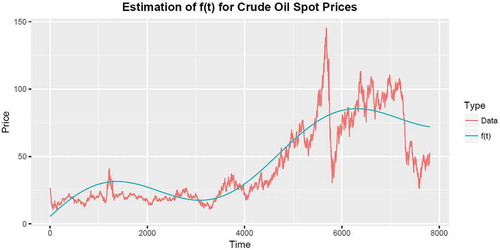
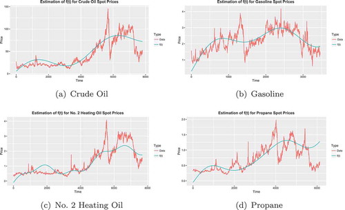
We focus on the one-factor model to explain our approach for estimating the model parameters. The data used in this section are obtained from the US Energy Information Administration and include future prices of Crude Oil (Light-Sweet, Cushing, Oklahoma) from 30 March 1983 to 6 December 2016 (8452 observations), Reformulated Regular Gasoline (New York Harbor) from 3 December 1984 to 31 October 2006 (5492 observations), Heating Oil (New York Harbor) from 2 January 1980 to 6 December 2016 (9262 observations) and Propane (Mont Belvieu, Texas) from 17 December 1993 to 18 September 2009 (3941 observations).
The parameters in the seasonality function (56) are estimated by fitting the function to the historical spot prices. The spot prices used include Crude Oil from 2 January 1986 to 12 December 2016 (7807 observations), RBOB Regular Gasoline from 11 March 2003 to 12 December 2016 (3460 observations), No. 2 Heating Oil from 2 June 1986 to 12 December 2016 (7683 observations) and Propane from 9 July 1992 to 12 December 2016 (6133 observations).
The accuracy of the fitting in Figure depends on the choice of the initial parameters ,
,
,
and
.
Figure 3. Seasonality is captured by the function defined in the following table. The best fit of
can be obtained by obtaining an optimal set of the
parameters.
6.1. Equivalent latent regression model
The de-seasonalised one-factor future price given by (58) can be written as
where ,
and
and
are given by
and is an independent random error distributed as
with zero mean and variance
.
Clearly, (63) belongs to the class of latent regression models since is not observable.
There is literature where this kind of problem is handled using expectation-maximisation (EM) algorithms (see Dempster, Laird, and Rubin (Citation1977)) to estimate the model parameters. The latent variable can be considered binary where in this case the EM algorithm would give estimates for a two-component normal mixture model. On the other hand,
can be allowed to be continuous between 0 and 1 with a beta distribution as in Tarpey and Petkova (Citation2010). The EM algorithm for estimating the model parameters in this case is more involved than for the two-component mixture model and more computationally challenging, but can be done nonetheless. Basically, the latent or unobserved
variables are imputed by their conditional expectation given the outcomes
. Our approach is adaptable to the latter approach through the Dynkin–Lamperti Theorem (see Gupta and Nadarajah (Citation2004)) where the unobserved variable follows a stable distribution defined on
with
and the observable variable
represents the log-returns of the future prices. The algorithm is applied to the joint likelihood of the response
. We assume the error
is independent of the latent predictor
. The joint density for
and
is given by
where is the
stable distribution,
denotes the normal distribution of a random variable
with mean
and variance
; and
is the variance of the outcome sample data. The marginal density of the response
is
Density (67) is an example of infinite mixture models used in ecological statistics (Fox, Negrete-Yankelevich, and Sosa (Citation2015)).
6.2. The EM algorithm
For a data set in (63). The log-likelihood is derived from (66) as
Since is not observable, the EM algorithm requires maximising the conditional expectation of the log-likelihood given the response vector
. That is
where at each iteration of the EM algorithm, the above conditional expectation is computed using the current parameter estimates. This current expectation-maximisation problem is similar to the problem handled in Tarpey and Petkova (Citation2010), which implies that a similar EM algorithm can be applied here. That is, suppose is a
dimension coefficient matrix where each of the
columns of
provides the intercept and slope regression coefficients for each of the
response variables. Then the design matrix is denoted by
whose first column consists of ones for the intercept and the second column consists of the latent predictors
. The multivariate regression model follows:
Moreover, and as indicated in Tarpey and Petkova (Citation2010), the likelihood for the multivariate normal regression model can be given as
The EM approach requires that we maximise the expectation of the logarithm of (71) conditional on with respect to
and
. This leads to the following optimal factors:
where and
.
To implement the EM method in the R programming language, we first highlight that there are a minor differences to bear in mind before implementing the algorithm as we explain in the following.
First and foremost, the density of the predicator in our case is from a stable distribution. Recall, in general, the densities of stable processes cannot be expressed analytically, which makes it difficult to compute the log-likelihood. However, with the help of inbuilt packages in R including and
, the log likelihood can be satisfactorily estimated using
to obtain the stable parameters of
, and
for its corresponding stable density.
Second, from the log-likelihood expression, we notice that we only require estimates of the conditional expectations of ,
and
with respect to the joint probability density given the response vector
.
On the other hand, we retain some of the steps in Tarpey and Petkova (Citation2010). The initial values for the regression parameters and
can be obtained from fitting a two-component finite mixture model or by a preliminary search over the parameter space. Initial values for
can be obtained using the sample covariance matrix from the raw data.
6.3. Data for the EM algorithm
The data used is stored in a data frame with three columns containing futures log-returns, spot price log-returns and binary data of 1’s and 0’s representing whether or not a jump has occurred within a given window size (see Table ). Table shows the estimated parameters as a result. The parameters were obtained from 5000 data points of crude oil log-returns arranged as in Table . We have displayed results from only two iterations because for large data sets the code tends to be slow in addition to suffering convergence issues. However, this can be improved and using faster machines.
Table 2. Estimation of parameters in the seasonality function
Table 3. Parameters obtained from maximum likelihood method
Table 4. A snapshot of the structure of the data used
The jump occurrence due to is determined by the method discussed in Lee and Mykland (Citation2008) (also see Maslyuka et al., Citation2013). That is the realised return at any given time is compared with a continuously estimated instantaneous volatility
to measure local variation arising from the continuous part of the process. The volatility
is estimated using a modified version of realised bipower variation calculated as the sum of products of consecutive absolute returns in the local window (see Barndorff-Nielsen & Shephard, Citation2004). Then, the jump detection statistic
testing for jumps in returns occurring at a time
within a window size
is calculated as the ratio of realised returns to estimated instantaneous volatility:
where at
represents the commodity spot price and
is estimated by
Care must be taken in choosing , it must be large enough to accurately estimate integrated volatility but small enough for the variance to be approximately constant. In other words,
should be large enough but smaller than
, the number of observations so that the effect of jumps on estimating instantaneous volatility disappears. Some authors recommend
to be computed as
, where
is the daily number of observations, whereas
is the number of days in the (financial) year. Moreover, the window size should be such that
with
. For high-frequency data, Lee and Mykland (Citation2008) recommend, for returns sampled at frequencies of
,
,
and
minutes, the corresponding values of
to be
,
,
and
. For our case, we shall choose
for crude oil future prices with returns sampled daily.
6.3.1. Detection of jumps in the data
The test statistic follows approximately a normal distribution when the data set has no jumps and its value becomes large otherwise. According to Lee and Mykland (Citation2008), the region for
is chosen based on the distribution of its maximum. For instance, suppose a particular interval
has no jumps and the distance between two consecutive observations in this interval is small (i.e.
), then the maximum should converge to the Gumbel variable:
where has a cumulative distribution function
,
is the set of
such that there is no jump in
and
,
are defined as
The test is conducted by comparing the standardised maximum of in (76) to the critical values from the Gumbel distribution where the null hypothesis of no jump is rejected when the jump statistic is given by
where is the
quantile function of the standard Gumbel distribution. Suppose
, then we reject the null hypothesis of no jump when
where
is such that
. That is
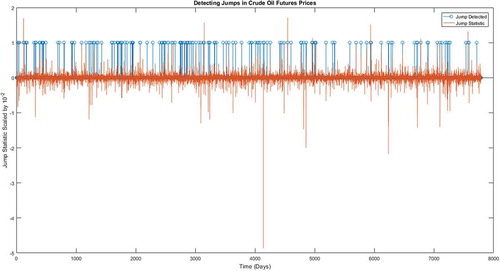
. Figure shows a graph of jumps detected in crude oil future prices where we have used 1’s to record a jump occurrence and
’s for no jump.
Figure 4. Detection of jumps in crude oil future prices.
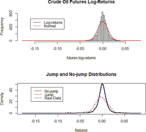
Figure 5. The large spikes in the jump statistic graph reflect the extreme events in the price where as the blue strips represent the smaller jumps that might go unnoticed. The former jumps are easily detected in returns yet the latter are not that visible.
7. Summary
We have shown that the affine property is attainable and applicable to generalised spot models. We considered a stochastic differential equation with the source of randomness as subordinated Brownian motion as a specific example to derive the futures price. Moreover, it has been argued in some existing literature that the likelihood function exists in integrated form for models with singular noise meanwhile for cases of partially observed processes, a filtering technique is required. However, the work presented in this paper provided a new approach of pricing commodity futures for models with latent variables using the maximum expectation-maximisation, without using any filtering. Our approach is easy to implement once the joint probability density is established. The numerical implementation of the two factor model is left for future work.
Correction
This article has been republished with minor changes. These changes do not impact the academic content of the article.
Acknowledgements
This work was supported by funds from the National Research Foundation of South Africa (NRF), the African Institute for Mathematical Sciences (AIMS) and the African Collaboration for Quantitative Finance and Risk Research (ACQuFRR), which is the research section of the African Institute of Financial Markets and Risk Management (AIFMRM), which delivers postgraduate education and training in financial markets, risk management and quantitative finance at the University of Cape Town in South Africa.
All the numerical results were generated using MATLAB and the Robust Analysis software package in R accessible at www.RobustAnalysis.com.
Additional information
Funding
Notes on contributors
M. Kateregga
M. Kateregga holds a Ph.D. in Mathematical Finance from the University of Cape Town. Michael is a Software Developer at Mira Networks in South Africa. His main interests include financial markets research and functional programming particularly Haskell.
Notes
1. The process is also interpreted as the first passage time of the stable process
.
References
- Applebaum, D. (2004). L´evy processes and stochastic calculus. Cambridge studies in advanced mathematics. Cambridge: Cambridge University Press.
- Barndorff-Nielsen, O. E., & Shephard, N. (2004). Power and bipower variation with stochastic volatility and jumps. Journal of Financial Econometrics, 2(1), 1–37. doi:10.1093/jjfinec/nbh001
- Black, F., & Scholes, M. (1973). The pricing of options and corporate liabilities. Journal of Political Economy, 81(3), 637–654. doi:10.1086/260062
- Bochner, S. (2012). Harmonic analysis and the theory of probability. Dover books on mathematics. Mineola, NY: Dover Publications.
- Crosby, J. (2008). A multi-factor jump-diffusion model for commodities. Journal of Quantitative Finance, 8(2), 181–200. doi:10.1080/14697680701253021
- Date, P., & Ponomareva, K. (2010). Linear and nonlinear filtering in mathematical finance: A review. IMA Journal of Management Mathematics, 22(3), 195–211. doi:10.1093/imaman/dpq008
- Dempster, A. P., Laird, N. M., & Rubin, D. B. (1977). Maximum likelihood from incomplete data via the EM algorithm. Journal of the American Statistical Association, 39, 1–38.
- Deng, S. (2000). "Stochastic models of energy commodity prices and their applications: Mean-reversion with jumps and spikes," Working Paper PWP-073, University of California Energy Institute.
- Duffie, D., Filipovi´C, D., & Schachermayer, W. (2003). Affine processes and applications in finance. Annals of Applied Probability, 13, 984–1053. doi:10.1214/aoap/1060202833
- Dumouchel, W. H. (1971). Stable distributions in statistical inference. The Journal of the American Statistical Association, 78(342), 469–477.
- Fama, E. F., & French, K. R. (1988). Permanent and temporary components of stock prices. The Journal of Political Economy, 96(2), 246–273. doi:10.1086/261535
- Fama, E. F., & Roll, R. (1968). Some properties of symmetric stable distributions. Journal of the American Statistical Association, 63(323), 817–836.
- Fox, G., Negrete-Yankelevich, S., & Sosa, V. (2015). Ecological statistics: Contemporary theory and application. Oxford: Oxford University Press.
- Fusai, G., & Roncoroni, A. (2007). Implementing models in quantitative finance: Methods and cases. Springer finance. Berlin, Heidelberg: Springer.
- G´omez-Valle, L., Habibilashkary, Z., & Martnez-Rodr`ıguez, J. (2017). A new technique to estimate the risk-neutral processes jump-diffusion commodity futures models. Journal of Computational and Applied Mathematics, 309, 435–441. doi:10.1016/j.cam.2015.12.028
- Gajda, J., & Wyłoman`Ska, A. (2012). Geometric Brownian motion with tempered stable waiting times. Journal of Statistical Physics 1, 148(2), 296–305. doi:10.1007/s10955-012-0537-3
- Grigelionis, B., Kubilius, J., Paulauskas, V., Statulevicius, V., & Pragarauskas, H. (1999). Probability theory and mathematical statistics: Proceedings of the seventh vilnius conference (1998), Vilnius, Lithuania, 12–18 August, 1998. Probability theory and mathematical statistics. TEV.
- Gupta, A., & Nadarajah, S. (2004). Handbook of beta distribution and its applications. Statistics: A series of textbooks and monographs. Abingdon: Taylor & Francis.
- Hicks, J. R. (1939). Value and Capital. Cambridge: Oxford University Press.
- Holt, D. R., & Crow, E. L. (1973). Tables and graphs of the stable probability density function. Journal of Research of the National Bureau of Standards, Section B, 77, 143–198. doi:10.6028/jres.077B.017
- Kateregga, M., Mataramvura, S., & Taylor, D. (2017). Parameter estimation for stable distributions with application to commodity futures log-returns. Cogent Economics & Finance, 5(1), 1318813. doi:10.1080/23322039.2017.1318813
- Keller-Ressel, M. (2008). Affine processes theory and applications in finance. ( PhD thesis), Technischen Universita¨t Wien, Vienna, Austria.
- Keller-Ressel, M., Schachermayer, W., & Teichmann, J. (2011). Affine processes are regular. Probability Theory and Related Fields, 151(3), 591–611. doi:10.1007/s00440-010-0309-4
- Keynes, J. M. (1930). A treatise on money, vol II. London, United Kingdom: Macmillan.
- Kyriakou, I., Nomikos, N. K., Pouliasis, P. K., & Papapostolou, N. C. (2016). Affine-structure models and the pricing of energy commodity derivatives. European Financial Management, 22(5), 853–881. doi:10.1111/eufm.12071
- Lee, S., & Mykland, P. A. (2008). Jumps in financial markets: A new nonparametric test and jump clustering. Review of Financial Studies, 21(6), 2535–2563.
- Maslyuka, S., Rotarub, K., & Dokumentovc, A. (2013). Price discontinuities in energy spot and futures prices. Monash Economics Working Papers 33-13, Monash University, Department of Economics.
- Meerschaert, M. M., & Straka, P. (2013). Inverse stable subordinators. Mathematical Modelling of Natural Phenomena, 8(2), 1–16. doi:10.1051/mmnp/20138201
- Miller, J. F. (1951). Moment-generating functions and laplace transforms. Journal of the Arkansas Academy of Science, 4(1), 16.
- Prokopczuk, M., Symeonidis, L., & Simen, C. W. (2015). Do jumps matter for volatility forecasting? Evidence from energy markets. Journal of Futures Markets, 20, 1–15.
- Rachev, S. (2003). Handbook of heavy tailed distributions in finance: Handbooks in finance. Handbooks in Finance. Amsterdam: Elsevier Science.
- Rouah, F., & Heston, S. (2015). The heston model and its extensions in VBA. Wiley Finance. Hoboken, NJ: Wiley.
- Samoradnitsky, G., & Taqqu, M. (1994). Stable non-gaussian random processes: Stochastic models with infinite variance. Stochastic modeling series. United Kingdom: Taylor & Francis.
- Schmitz, A., Wang, Z., & Kimn, J.-H. (2014). A jump diffusion model for agricultural commodities with bayesian analysis. Journal of Futures Markets, 34(3), 235–260. doi:10.1002/fut.21597
- Schwartz, E. S. (1997). The stochastic behaviour of commodity prices: Implications for valuation and hedging. The Journal of Finance, 52(3), 923–973. doi:10.1111/j.1540-6261.1997.tb02721.x
- Schwartz, E. S., & Smith, J. E. (2000). Short-term variations and long-term dynamics in commodity prices. Management Science, 46(7), 893–911. doi:10.1287/mnsc.46.7.893.12034
- Tarpey, T., & Petkova, E. (2010). Latent regression analysis. Statistical Modelling, 10(2), 133–158. doi:10.1177/1471082X0801000202
- Yang, J., Lin, B., Luk, W., & Nahar, T. (2014). Particle filtering-based maximum likelihood estimation for financial parameter estimation. In 2014 24th International Conference on Field Programmable Logic and Applications (FPL), 1–4.
- Zolotarev, V. (1986). One-dimensional stable distributions. Translations of mathematical mono-graphs. Providence, Rhode Island, United States: American Mathematical Society.
- Zolotarev, V. M. (1964). On the representation of stable laws by integrals. Trudy Matematicheskogo Instituta Imeni V.A. Steklova, 71, 46–50.
- Zolotarev, V. M. (1980). Statistical estimates of the parameters of stable laws. Banach Center Publications, 6(1), 359–376. doi:10.4064/-6-1-359-376
Appendix A
Proof for Theorem 5.1
By applying Itô’s formula to , it is readily seen that
where and the future price with maturity date
is given by (see (see Schwartz (Citation1997))
Theorem 4.5 suggests an explicit representation of (81) is attainable and it can be deduced by considering first, the continuous case . Suppose a continuous mean-reverting model given by
The corresponding affine forms of the coefficients according to Theorem 4.5 yield:
Since is regular affine and
is constant for all
, then we have
where the functions ,
and
satisfy the set of Riccati equations:
where . The solution set to the system of Riccati equations is given by
Using (84) where , one can easily deduce
leading to the price of a commodity future price under a continuous model framework. Capitalising on the affine nature of
and Theorem 4.6, we deduce the representation for
as:
where the volatility is a constant and the system of Riccati equations takes the form
Consequently, the solution set is directly deduced from (88) (90) to obtain
Setting yields
The required result follows by substituting the Lévy exponent from (41).
Justifications for theorem 5.3
where coefficients satisfy
Note that to ensure that the futures price is positive real, the values of have to be chosen carefully which in this case it could be
.
The factor is defined as
Finally, the integrating factor is such that
We provide the proof using the following proposition and subsequent lemmas.
Proposition 8.2 The mean and variance of the model (60)–(61) are given by
Moreover, their affine forms can be given as linear models of both and
:
where
As a consequence, we deduce the following system of Riccati equations:
where with initial conditions
,
,
. The solutions take the form:
Proof 8.3 This follows from the applications of Theorems 4.5 and 4.6.
To obtain the solution to the Riccati, Equation (114) is not trivial. However, a similar problem has been handled in Kyriakou et al. (Citation2016), see Lemmas 8.4 and 8.6.
Lemma 8.4 Consider Proposition 8.2 and let be such that it satisfies
then the solution to (114) can be expressed by
Moreover, the general solution to (114) takes the form
where satisfies
with the general solution given by
where is an integrating factor and
is the constant of integration.
Proof 8.5 Claim (118) is verified by differentiating with respect to and relating it to (117) and (115):
Similarly, (119) is verified by substitution into (114) and relating it to (122) resulting into
from which (120) follows. The general solution to (120) is obtained using the integrating factor
Lemma 8.6 A representation of the solution to (114) is given by
where the constant of integration is determined by applying
:
Proof 8.7 The function can be expressed in the form (see Kyriakou et al. (Citation2016)):
Functions and
in (125) and (116), respectively, can be re-written as
where the integrating factor introduced in (124) and its integral are given by
Finally, the constant of integration (126) can be re-written as
This completes the proof.