Modelling the determinants of government expenditure in Nigeria

Abstr

In Nigeria, the government activities vis-à-vis public expenditure has grown rapidly both in absolute, relative and as a share of GDP over the years. These growths in government expenditure have been due to certain factors which are believed to have significant effect on the fiscal operation of the country. These perceived implications of government expenditure expansion on the economy necessitate the need to understand factors that are responsible for the growth in government expenditure size. For that, the study employs a slightly modified version of Wagner’s law by incorporating new variables such as oil revenue, trade openness, public debt, exchange rate, oil price, taxation and inflation—to examine their effect on government expenditure size. The study uses time series data for Nigeria spanning between 1970 and 2017. Time series data were analysed using Autoregressive Distributed Lag (ARDL) model. The findings of the study reveal that oil revenue, GDP, population, trade openness, oil price, taxation and inflation are important determinants of the size of Nigeria’s government expenditure. The study recommends among others that the revenue base of the country should be diversified beyond oil sector, strengthening of fiscal and monetary policies to ensure stability in price level and exchange rate, the use of fiscal rule through excess crude oil account should also be strengthened to create buffer against fluctuation in oil price and as well appropriate population reduction policies should be undertaken to curtail rapid population growth.

Keywords:

• ARDL
• government expenditure
• Nigeria
• Wagner’s law

JEL Classification Code:

• C22
• H11
• H50.

PUBLIC INTEREST STATEMENT

In recent times, rising government expenditure has become a major source of public concern in Nigeria. Expansion in government expenditure has created serious challenges for several government policies in the country, particularly budget control and debt management. In this context, the policy drives for an efficient management of government spending towards ensuring sustainable development create the need for better understanding of the factors responsible for the overall growth in government expenditure of Nigeria. These determinants form crucial factors in managing fiscal imbalances in a developing nation like Nigeria, particularly when the country still finds itself grappling with the issues of development. Thus, this paper investigates the determinants of government expenditure in Nigeria using time series data spanning between 1970 and 2017. The findings from the study reveal that oil revenue, tax revenue, oil price, economic growth, population, inflation and trade openness are the major determinants of growth in the size of Nigeria’s government expenditure in Nigeria.

1. Introduction

In majority of the developing countries, government is seen as an instrument of change and, hence, the size of government expenditure reveals the magnitude of government involvement in the economy. The shift in the role of government from traditional functions such as provision of security, administration and law and order to direct intervention in income generating activities like capital investment and distributive role like subsidies and transfers have significantly expanded the scope of governments in many countries across the globe.

The major objective of government is therefore to promote societal welfare by means of appropriate economic, political, social and legal programmes. These programmes, however, have led to expansion in public expenditure size particularly in the developing economies like Nigeria with a weak and uncompetitive private sector. Wagner (1883) was assumed to be the first economist who linked economic progress and population growth as the major factors responsible for the growth of government expenditure using the experience of industrialized welfare states. This was later named as Wagner’s law and it has spawned volume of theoretical and empirical debates attempting to point out factors causing growth in government expenditure of various countries (see Bagdigen & Cetintas, 2004; Bird, 1971; Dreher, Strum, & Upsprung, 2008; Durevall & Henrekson, 2011; Eterovic & Eterovic, 2012; Facchini & Melki, 2013; Jin & Zou, 2002; Kumar, Webber, & Fargher, 2012; Magazzino, Giolli, & Mele, 2015; Musgrave, 1969; Shonchoy, 2010; Shelton, 2007; Peacock & Wiseman, 1961).

The continued debate on the determinants of government size becomes necessary because those determining factors are needed not only for managing fiscal imbalances but also to encourage stability in the economy (Aladejare, 2019; Uchenna & Evans, 2014). This becomes more relevant in a country like Nigeria where despite large expansion in government expenditure both in real and as a share to GDP (see Figures 1 and 2), development challenges such as high poverty, unemployment, death of necessary infrastructures and insecurity in economy and society remain increasingly persistent.

Figure 1. Nigeria’s total government expenditure (1970–2017).

Trend of Nigeria’s central government expenditure where the horizontal axis shows six years in average. Computed from Statistical Bulletin of the CBN, 2017.

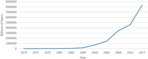
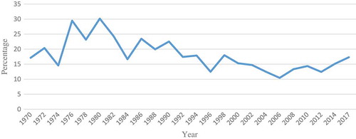
Figure 2. Share of total government expenditure in GDP (1970–2017).

Trend of Nigeria’s central government expenditure share to GDP where the horizontal axis shows two years in average. Computed from Statistical Bulletin of the CBN, 2017.

Therefore, this paper aims to examine empirically the factors responsible for the growth of government expenditure in Nigeria within the framework of Wagner’s law. Previous studies across the globe have revealed different factors causing expansion in government expenditure. For instance, public debt is found to be a significant factor influencing the growth of government expenditure (Eterovic & Eterovic, 2012), corruption (Mauro, 1998) and population and urbanization (Ofori-Abebrese, 2012; Shelton, 2007; Shonchoy, 2010). While other studies have identified inflation (Ezirim, Muoghalu, & Elike, 2008) and democracy (Obeng & Sakyi, 2017) as the main determinants of government expenditure, other notable factors include foreign aid (Heller, 1975; Njeru, 2003), globalization (Dreher et al., 2008) and trade openness (Cameron, 1978), among others.

There are also quite a number of studies that investigated the determinants of government expenditure in Nigeria during the past decades (see Abeng, 2005; Akanbi, 2014; Aladejare, 2019; Aregbeyen & Akpan, 2013; Okafor & Eiya, 2011; Taiwo, 1989; Ukwueze, 2015); however, we observed that these studies biased their analyses towards common factors, leading to the exclusion of several variables like oil price, oil revenue, trade openness, taxation, exchange rate, among others, which have shown to be significant in various studies for other countries and are believed to have potential role in explaining the growth of public expenditure in Nigeria. Hence, this paper attempts to move the debate further by incorporating previously omitted variables in the analysis of the determinants of the size of government expenditure in Nigeria. Further, the present study counters the empirical debates on the determinants of government expenditure especially their robustness by employing more than one measure of government expenditure and economic growth which is considered as a headway in this area of research.

The subsequent sections of this paper are organized in six sections as follows: following the introduction (Section 1), Section 2 discusses government expenditure profile in Nigeria. Similarly, Section 3 provides review of literature. Respectively, methodology and results and discussion are treated in Sections 4 and 5, followed by conclusion and policy recommendations in the last section.

2. Government expenditure profile

The trend of public expenditure in Nigeria over the years has been characterized by steady and continuous increase in the expenditure side of the budget as presented in Figure 1. Government expenditure was ₦314.41 billion on average between 1960 and 1970 but rose to ₦5972.90 billion between 1971 and 1980 representing 1799.7% growth in government expenditure during the decade of 1970s (CBN, 2017). The expansion can be associated with the discovery of oil in the early 1970s that led to unprecedented increase in Nigeria’s revenue. Additionally, government budgeted large monies for reconstruction after the 1960s civil war that lasted for about 30 months. The country also embarked on increase in spending on priority sectors to provide an enabling environment needed to accelerate sustainable growth and development.

Besides, government expenditure was ₦11,188.42 billion on average between 1981 and 1985 representing the growth rate of 87.3% (CBN, 2017). Furthermore, public expenditure exhibited upwards trend despite countless efforts by government to reduce its expenditure particularly through the structural adjustment program (SAP) in 1986 which focused on short-term and medium-term policy reforms to structurally adjust the economy. Public expenditure continued to maintain steady and upwards trend from 1986 to 1991. Total government expenditure was ₦11,413.7 billion in 1986 but by 1990, it slightly increased to ₦66,584.4 billion representing 10% increase (CBN, 2017). This development could be attributed to the volatile revenue base of government and large fiscal deficits which resulted to decrease in government expenditure. Aregbeyen and Akpan (2013) posit that after the implementation of SAP, which marked the post-liberalization era in 1986, strict measures were put in place to curb government spending. This includes reduction in wage bills, reduction in government subsidies, limiting or delaying investment projects and privatization/commercialization. That has indeed reflected in the expenditure pattern as government expenditure growth rate was on average 31.1% between 1986 and 1991 compared with the growth rate of 87% between 1981 and 1985.

However, in the period 1991–1995, government made effort to reduce inflation rate by avoiding large budgetary deficits, which made government expenditure more cost-effective and consistent with the nation resources. In fact, public expenditure reduced from ₦191,228.90 billion in 1993 to ₦160,893.20 billion in 1994 representing −15.9% growth rate in government expenditure (CBN, 2017).

Lastly, from 2000 to 2017, government expenditure continues to increase unabated. Throughout the period, government expenditure maintained a rising trend. Public expenditure was ₦701,059.40 billion and rose immensely to ₦4,813,380.00 billion from 2000 to 2016, respectively. Average growth rate of government expenditure was 19.2% between 2001 and 2010 (CBN, 2017). Public expenditure has been continuously increasing in this period because of the increased demand for the provision of socioeconomic services due to the population growth, increase in the flow of revenue from the production and sales of crude oil as a result of high price of crude oil in the international market, expenditure on election and the desire of policymakers and political leaders to meet the aspiration of citizens as well as to fulfil election promises.

Furthermore, in order to have more insight on the trend of government expenditure in Nigeria, it is paramount to highlight the share of government expenditure in GDP of Nigeria over the years. Figure 2 depicts the graphical presentation of the share of government expenditure in GDP of Nigeria between 1970 and 2017. It can be seen that the decade of 1970 recoded the highest share of expenditure in GDP accounting for 29% in 1976. This can be attributed to the oil boom witnessed during the period which significantly influenced government decision regarding spending and the efforts made by government in rebuilding the economy after the civil war that lasted for about 30 months. Furthermore, there was steady decline from 1985 in which the value stood at 19% and continued to decline in a fluctuating form until 1996 where it rose from 12% to 29% in 1999 when the country returned to democratic rule. In 2000, it declined to 15.3% and rose to 21% in 2001. Since then, government maintained an average share to GDP of about 15% during the period between 2002 and 2017. In general, the trend has fluctuated over the years showing the effect of various policy programmes of government.

3. Literature review

The earliest theory of public expenditure could be traced to Wagner (1883), a German political economist who postulated a model of public expenditure growth in an attempt to generalize and explain the changes in levels of public expenditure. He comes up with “the law of increasing state activity”. He hypothesizes that as the economy develops over time, it is accompanied with an intensive and extensive increase in activities and functions of the government which in turn leads to growth in government expenditure.

Brown and Jackson (1994) sum up Wagner’s law as the law of increasing expansion of public and particularly state activities become for the fiscal economy the law of the increasing expansion of fiscal requirements. Both the state’s requirements grow and, often even more so, those of local authorities, when administration is decentralized and local government well organized. Recently, there has been a marked increase in Germany in the fiscal requirements of municipalities, especially urban ones. That law is the result of empirical observation in progressive countries at least in western European civilizations: its explanation, justification and cause is the pressure for social progress and the resulting change in the relative spheres of private and public economy, especially compulsory public economy. Financial stringency may hamper the expansion of state activities, causing their extent to be conditioned by revenue rather than the other way round, as is more usual. But in the long-run the desire for development of a progressive people will always overcome these financial difficulties” (p. 174).

Furthermore, Sagarik (2014) explained Wagner’s law of expanding state activity in three ways. First, industrialization and modernization would lead to a great amount of public activities as a substitute for private ones. There is more need for public protective and regulative activity. In addition, the greater division of labour and urbanization accompanying industrialization would require higher expenditure on contractual enforcement, as well as on law and order, to guarantee the efficient performance of the economy. Wagner’s law, thus, predicts that industrialization is accompanied by an increase in public expenditure as a share of GDP. Wagner’s law attempts to explain the state’s increasing actual behaviour, particularly regarding public expenditure.

Second, Wagner (1883) argues that the growth in real income would facilitate the relative expansion of welfare expenditure. The degree of economic development, measured through the GDP per capita, influences the availability of economic resources for the purposes of public spending. This could be considered as the core of Wagner’s law, as economic growth has been the focus or goal of development for decades and it plays an important role in much of the public policy literature.

Finally, Wagner (1883) believes that “natural monopolies” are best managed by the public sector. He cites the case of railroads as a natural monopoly and points out that the private sector would be unable to raise huge finances and run such natural monopolies efficiently. This could also imply that an increase in the rate of population growth would raise the need for public services such roads, schools, hospitals, security, among others, which also leads to increased public spending.

There seems to be a reasonable consensus in the literature that Wagner’s law should be interpreted as predicting an increasing relative share of the public expenditure in the total economy as per capita real income grows.

Wagner’s law has been further advanced by many scholars of public finance (Bird, 1971; Goffman and Mahar, 1971; Gupta, 1967; Mann, 1980; Musgrave, 1969; Pryor, 1968). Many researchers have adopted different versions of the law advanced by these scholars to examine the impact of economic growth and other variables on public expenditure using variety of methodological tools with different data set (time series, panel and cross sectional) and obtained divergent and mixed results.

For instance, income or mostly proxy as GDP is one of the earliest and probably most frequently mentioned determinants of government expenditure. There is volume of studies both in developed and developing countries that provide empirical evidence in support of Wagner’s hypothesis (see Gyles, 1991; Adamu & Hajara, 2015; Facchini & Melki, 2013; Jalles, 2019; Kumar et al., 2012; Magazzino et al., 2015; Michas, 1974; Obeng & Sakyi, 2017; Sagdic, Sasmaz, & Tuncer, 2019). Thus, the implication of the above findings is that the level of economic growth and development of a country has a significant influence on public expenditure size. Conversely, there are some empirical studies that do not find support for Wagner’s hypothesis. Some of these studies include Bagdigen and Cetintas (2004), Durevall and Henrekson (2011), Hayo (1994), Henrekson (1993), Pelawaththage (2019), and Singh and Sahni (1984). All these studies found negative association between national income and public expenditure. This means that overall growth and development is not always accompanied by expansion in the size of government expenditure.

Public revenue is also another factor that has been hypothesized as an important variable influencing the growth of public expenditure. The revenue–spend hypothesis, put forward by Friedman (1978), that changes in government revenue brings about changes in government expenditure. It is characterized by unidirectional causality running from government revenue to government expenditure. There are some empirical studies that validate this hypothesis using data for both developed and developing countries, some of these studies include Athanasenas, Katrakilidis and Trachanas (2014), Aworinde (2013), Blackley (1986), Bolat (2014), Dizaji (2014), Moalusi (2004), Mutascu (2016), Mutascu (2017) and Saunoris (2015). The implication of revenue–spend hypothesis is that improvement in public revenue would always be accompanied by expansion in the size of government expenditure. This may be devastating especially for countries with unstable revenue.

The spend–revenue hypothesis, advanced by Peacock and Wiseman (1961), states that changes in public expenditure bring about changes in public revenue. This hypothesis has been supported by several empirical studies using data for different countries (Narayan & Narayan, 2006; Parida, 2012; Richter & Dimitrios, 2013; Saunoris & Payne, 2010; Zapf & Payne, 2009). The spend–tax hypothesis places expenditures ahead of revenues. The effect could be scary if proper policies are not devised to cushion the escalation of budget deficit with consequence of shifting repayment burden on the future tax payers.

More so, the fiscal synchronization hypothesis, developed by Musgrave (1966), states that citizens compare the marginal benefits and marginal costs of government services in making fiscal policy decision. Therefore, it is characterized by bidirectional causality between government revenue and expenditure. Some empirical studies have supported this hypothesis like Baharumshah, Jibrilla, Sirag, Ali and Muhammad (2016) find support for fiscal synchronization hypothesis using data for South Africa. Similar evidence is found by Phiri (2016). Contrary, Ali and Amin (2018) find support for neutrality hypothesis indicating that there is absence of causality between the fiscal variables which signifies that revenue and expenditure are independent of each other.

There are also some studies that investigated the influence of public debt servicing on public expenditure. Aregbeyen and Akpan (2013) using disaggregated data for Nigeria ranging from 1960 to 2010 find that debt servicing reduces all forms of government expenditure in Nigeria. Okafor and Eiya (2011) find positive association between public debt and government expenditure expansion in Nigeria.

Another empirical study by Rodrik (1998) shows a positive relationship between government debt and government size. Additionally, Dreher et al. (2008) applying panel data for 108 countries using pooled least square panel find a significant nexus between government debt and government size. Equally, Okafor and Eiya (2011) and Aregbeyen and Akpan (2013) found the same evidence using Nigerian data for the period 1999 and 2008 and 1970 and 2010, respectively. It is truism because traditionally debts are contracted to finance developmental projects especially in developing economies.

Inflation is another variable that is assumed to be responsible in influencing the growth of public expenditure. Inflationary pressure is indeed a crucial macroeconomic problem facing most countries in the world particularly developing economies. For instance, Ezirim et al. (2008), using time series data for US economy, reveal that there is a long-run relationship between inflation and public expenditure. Inflation has also been found influential on Pakistan public expenditure in a study by Attari and Javed (2013) applying econometric techniques using annual data. Similar result is found by Olayungbo (2013) using time series data for Nigeria, the paper found a long-run equilibrium relationship between government expenditure and inflation. Conversely, there are some empirical studies that established insignificant relationship between inflation and public expenditure growth (Eterovic & Eterovic, 2012; Jin & Zou, 2002; Okafor & Eiya, 2011; Rodrik, 1998). This may be true especially for countries that have sound macroeconomic environment which promotes price stability.

More so, there are many empirical studies that investigate the influence of population on public spending. For instance, Goffman and Mahar (1971), in their empirical study, note that the age structure of the population has been a dominant factor in public expenditure growth in developing nations. Thorn (1972) show that the rapidity of increase, urbanization and life expectancy are possible underlying explanations for public sector expansion. Empirical studies by Epifani and Gancia (2009), Abeng (2005), Okafor and Eiya (2011), Aregbeyen and Akpan (2013), Ofori-Abebrese (2012) and Obeng and Sakyi (2017) reveal that increase in population contributes immensely in public sector expansion.

There are also studies that find a positive and significant association between trade openness and the size of government expenditure (Cameron, 1978; Rodrik, 1998; Shelton, 2007). The results can be explained as exposure to foreign shocks through trade openness increases government expenditure. In another study by Aladejare (2019), the study applied Nigeria data set spanning between 1970 and 2016 and revealed that oil price, price level and oil revenue are the major determinants of government expenditure.

It is very clear from the reviewed literature that numerous studies have queried about what actually influence public expenditure, mostly from the developed economies to emerging and developing countries’ counterpart. However, the studies focused either on economic, political and institutional or demographic factors. Some of these factors thought to shift the demand or supply of public spending. Therefore, a change in these variables brings about a corresponding change in the demand and supply of public goods.

4. Econometric methodology

4.1. Theoretical strategy

Numerous propositions have been advanced to explain the growth of government expenditure. Most notable is the one associated with Wagner (1883). As noted earlier, Wagner basic hypothesis is that increase in per capita income is accompanied by increase in government expenditure. This is symbolically expressed in the following equation:

(1) $Gf(Y)$(1)

where G stands for government expenditure and Y represents income. Wagner’s law has been adopted and modified in various functional forms for the past decades in analysing the causes of growth in government expenditure. Notably among them are studies by Goffman and Mahar (1971a), Gupta (1967), Mann (1980), Musgrave (1969) and Peacock and Wiseman (1961). The present study proceeds to formulate the model of public expenditure by modifying Equation (1) to incorporate other relevant variables. We begin to assume that the desired level of public expenditure (G*) is linearly dependent on level of income (Y). We assume the following adjustment within the spirit of Gafar (1975). Since it takes time for the actual level of government expenditure (G) to adjust in accordance with new income level (Y), we then assume the following adjustment process in the following equation:

(2) $G_t-G_{t-1}=\theta (G\ast -G_{t-1}),0\le \lambda \le 1$(2)

where λ stands for the adjustment term and other variables remained as previously defined. Substituting and rearranging Equation (1) in Equation (2), we get the following equation as

(3) $G_t=\lambda a+\lambda b{Y}_t+(1-\lambda )G_{t-1}=A_0+A_1{Y}_t{A}_2{G}_{t-1}$(3)

If λ = 1, that is to say, if the adjustment is instantaneous, Equation (3) reduces to

(4) $G_t=G_t\ast ie{G}_t=a+b{Y}_t$(4)

Equation (4) is the functional form that is usually estimated as Wagner’s law. We can therefore modify Equation (4) by incorporating other relevant variables identified in the literature in order to estimate the determinants of government expenditure.

4.4 Estimation strategy

It has been well documented in empirical literature that no meaningful econometric analysis can be achieved using time series data without properly checking for the unit root series of the variables. In fact, it is the unit root pattern of the variables that would to a large extent determine the appropriate techniques to be applied in data analysis. There are numerous techniques for the determination of stationarity of time series data, but for the purpose of this study, Augmented Dickey–Fuller (ADF) test developed by Dickey and Fuller (1981) and Philips–Perron (PP) test proposed by Philips and Perron (1988) are applied because they are the most common and simple among all other techniques. Besides that, they are also robust and have the capacity to remove autocorrelation from the model.

Further, the study applied the autoregressive distributive lag (ARDL) model approach to co-integration, which was popularized by Pesaran and Shin (1995), Pesaran and Smith (1997) and Pesaran, Shin and Smith (2001). This approach is chosen over other approaches because of its several advantages. First, ARDL approach can be applied without taking into account whether the explained variables are I(1) or I(0). This implies that the combination of I(1) and I(0) or mutually co-integrated are possible using ARDL approach. Second, it yields unbiased estimates in regression analysis and can be applied on small sample data while the Johansen co-integration requires large sample data for validity. Third, the ARDL approach to co-integration enables estimation using ordinary least squares method once the lag of the model is identified. Furthermore, Tang (2006) stresses that the ARDL approach is also applicable when the explanatory variables are endogenous and it has power to correct for serial correlation. Lastly, ARDL approach allows estimation of different variables with dissimilar optimal number of lags.

According to Pesaran and Smith (1997), the ARDL approach to co-integration requires the following two steps: First, to determine the existence of any long-run relationship among the variable of interest using F-test. Second, estimate the coefficients of the long-run relationship and determine their respective values, followed by the estimation of the short-run parameters of the variables with the aid of error correction representation of the ARDL model. The error correction mechanism (ECM) would also help in understanding the speed of adjustment to equilibrium.

4.3. Model specification

4.3.1. Model 1: Nominal government expenditure

The model in Equation (4) can be transformed by including other important variables as expressed in Equation (5).

(6) $\begin{array}{rl}& lnG{E}_t={\beta }_0+{\beta }_{1}lnGD{P}_t+{\beta }_{2}lnOIL{R}_t+{\beta }_{3}lnDEB{T}_t+{\beta }_{4}lnPO{P}_t\\ & +{\beta }_{5}IN{F}_t+{\beta }_{6}TO{P}_t+{\epsilon }_t\end{array}$(6)

where GE is the government expenditure, GDP is the gross domestic product, OILR is the oil revenue, DEBT is the public debt, POP is the population, INF is the inflation and TOP is the trade openness.

β₀ is the coefficient of the lagged-dependent variable. It provides the rate of self-perpetuating adjustment of the total government expenditure. β₁ … β₆ are coefficients of the explanatory variables expressed in logarithm, except for inflation and trade openness—which are used to explain the behaviour of growth in government expenditure size.

In econometric analysis, the description and measurement of variables of interest remain a critical task. This is because proper variables need to be selected and measured in order to have a meaningful result. Table 1 shows how each variable in the model is measured and where the data are sourced.

Table 1. Description of variables and sources of data

Variable	Description and measurement	Source
Government expenditure	Nominal total government expenditure of the central government of Nigeria	CBN
GDP	Nominal GDP	CBN
Oil revenue	Total federally collected revenue from oil	CBN
Public debt	Total debt stock of the central government	CBN
Trade openness	The degree of trade openness is proxy using the ratio of volume of trade (import plus export) to GDP	CBN
Population	Total population	WDI
Inflation	Inflation rate	WDI

Notes: CBN stands for Central bank of Nigeria and WDI stands for World Development Indicators by World Bank. All data are measured in nominal form and in local currency (Naira) and converted into natural logarithms except for inflation and trade openness that are in percentages and ratio, respectively. Source: Drawn by author.

The first step in ARDL approach is to estimate the conditional ARDL which is specified for model 1 and expressed in the following equation as

(7) $\begin{array}{rl}& \mathrm{\Delta }lnG{E}_t={\beta }_0+{\beta }_{1}lnG{E}_{t-1}+{\beta }_{2}lnGD{P}_{t-1}+{\beta }_{3}lnOIL{R}_{t-1}+{\beta }_{4}lnDEB{T}_{t-1}\\ & +{\beta }_{5}PO{P}_{t-1}+{\beta }_{6}IN{F}_{t-1}+{\beta }_{7}TO{P}_{t-1}+\sum _{i=1}^{\rho }{\theta }_{i1}\mathrm{\Delta }lnG{E}_{t-1}+\sum _{i=1}^{\rho }{\theta }_{i2}\mathrm{\Delta }lnGD{P}_{t-i}+\sum _{i=1}^{\rho }{\theta }_{i3}\mathrm{\Delta }lnOIL{R}_{t-i}\\ & +\sum _{i=1}^p{\theta }_{5i}\mathrm{\Delta }lnDEB{T}_{t-i}+\sum _{i=1}^p{\theta }_{6i}\mathrm{\Delta }lnPO{P}_{t-i}+\sum _{i=1}^p{\theta }_{7i}\mathrm{\Delta }IN{F}_{t-i}+\sum _{i=1}^p{\theta }_{8i}\mathrm{\Delta }TO{P}_{t-i}+{\epsilon }_t\end{array}$(7)

where ß₀ is the drift component, µ_t is the stochastic error term, ∆ is the first different operator, the parameters ß_0–8 denote the long-run parameters, while θ_1–8 represents short-run parameters of the model to be estimated through the error correction framework of ARDL. GE is the natural log of total government expenditure, lnGDP is the natural log of gross domestic product, lnOILR is the natural log of oil revenue, lnDEBT is the natural log of public debt, lnPOP is the natural log of population, INF is inflation and TOP is trade openness, ρ is the optimal lag length and ß_1–7 are the coefficients to be estimated in the model.

The next step is to apply Equation (7) to estimate the hypothesis that there is no co-integration relationship among the variables against the alternative hypothesis that there is long-run relationship between the variables. This is specified as

$H_0:{\beta }_1={\beta }_2={\beta }_3={\beta }_4={\beta }_5={\beta }_6={\beta }_7=0$

$H_1:{\beta }_1\ne {\beta }_2\ne {\beta }_3\ne {\beta }_4\ne {\beta }_5\ne {\beta }_6\ne {\beta }_7\ne 0$

β₁–β₇ remain as previously defined.

Pesaran et al. (2001) generate and present appropriate critical values according to the number of independent variables included in the model. In this regard, the calculated F-statistics is compared with two sets of critical values developed on the ground that the explanatory variables are I(d) (where 0 ≤ d ≤ 1). The lower critical values assume that all the variables are I(0) while the upper assumed that they are I(1). The criterion for the F-statistic is, if the calculated F-statistic is greater than upper critical value, then null hypothesis of no long-run relationship is rejected. On the other hand, if the F-statistic is less than lower bound, then the null hypothesis of no co-integration would be accepted. Furthermore, if F-statistic lies within the lower and upper critical bounds, then the result is inconclusive (Pesaran & Smith, 1997). To obtain the long-run coefficient, Equation (7) is specified as

(8) $\begin{array}{rl}& lnG{E}_t={\beta }_0+\sum _{i=0}^p{\beta }_{0}lnG{E}_{t-1}+\sum _{i=1}^{p_1}{\beta }_{1}lnGD{P}_{t-1}+\sum _{i=1}^{p_2}{\beta }_{2}lnOIL{R}_{t-1}+\sum _{i=0}^{p_3}{\beta }_{3}lnDEB{T}_{t-1}\\ & +\sum _{i=0}^{p_4}{\beta }_{4}lnPO{P}_{t-1}+\sum _{i=0}^{p_5}{\beta }_{5}IN{F}_{t-1}+\sum _{i=0}^{p_6}{\beta }_{6}TO{P}_{t-1}+{\mu }_t\end{array}$(8)

After establishing the long-run co-integration, the short-run model of the ARDL can be specified in the following equation:

(9) $\begin{array}{rl}& \mathrm{\Delta }lnG{E}_{t-i}={\beta }_0+\sum _{i=1}^p{\beta }_1\mathrm{\Delta }lnG{E}_{t-i}+\sum _{i=1}^p{\beta }_{2}ln\mathrm{\Delta }GD{P}_{t-i}++\sum _{i=1}^p{\beta }_{3}ln\mathrm{\Delta }OIL{R}_{t-i}+\sum _{i=0}^p{\beta }_{3}ln\mathrm{\Delta }DED{T}_{t-i}\\ & +\sum _{i=0}^p{\beta }_5\mathrm{\Delta }lnPO{P}_{t-i}+\sum _{i=0}^p{\beta }_6\mathrm{\Delta }IN{F}_{t-i}+\sum _{i=0}^p{\beta }_7\mathrm{\Delta }TO{P}_{t-i}+\theta EC{M}_{t-i}+{\epsilon }_t\end{array}$(9)

where β₁–β₇ remain as previously defined. While ∆ represents coefficients of short-run dynamic to be estimated, θ represents the speed of adjustment, ECM is the error correction term and all the remaining variables remain as previously defined.

4.3.2. Model 2: Real government expenditure as a share of GDP

In order to provide robust findings, another measure of government expenditure and economic growth is applied with different sets of independent variables. The model is presented in the following equation:

(10) $\begin{array}{rl}& GE/GD{P}_t={\alpha }_0+{\alpha }_{1}RGDP{G}_t+{\alpha }_{2}REXC{H}_t+{\alpha }_{3}POP{G}_t\\ & +{\alpha }_{4}lnTAX{R}_t+{\alpha }_{5}lnOIL{P}_t+{\alpha }_{6}TO{P}_t+{\epsilon }_t\end{array}$(10)

where GE/GDP is the real government expenditure as a share of real GDP, RGDPG is the real GDP growth rate, REXCH is the real effective exchange rate, POPG is the population growth, POPG is the population growth, TAXR is the tax revenue, OILP is the oil price and TOP is the trade openness.

β₀ is the coefficient of the lagged dependent variable. It provides the rate of self-perpetuating adjustment of the total government expenditure α₁–α₆ which are coefficients of the explanatory variables expressed in logarithm, except for inflation, real exchange rate, population growth, real GDP growth, real government expenditure as a share of real GDP and trade openness—which are used to explain the behaviour of growth in government expenditure. All other variables remain as previously defined.

To obtain the long-run coefficient for model 2, the specification equation is specified as

(11) $\begin{array}{rl}& lnGE/GD{P}_t={\alpha }_0+\sum _{i=0}^p{\alpha }_{0}lnGE/GD{P}_{t-1}+\sum _{i=1}^{p_1}{\alpha }_{1}lnRGDP{G}_{t-1}+\sum _{i=1}^{p_2}{\alpha }_{2}lnREXC{H}_{t-1}\\ & +\sum _{i=0}^{p_3}{\alpha }_{3}lnPOP{G}_{t-1}+\sum _{i=0}^{p_4}{\alpha }_{4}lnTAX{R}_{t-1}+\sum _{i=0}^{p_5}{\alpha }_{5}lnOIL{P}_{t-1}+\sum _{i=0}^{p_6}{\alpha }_{6}TO{P}_{t-1}+{\mu }_t\end{array}$(11)

After establishing the long-run co-integration, the short-run model of the ARDL can be specified in the following equation:

(12) $\begin{array}{rl}& \mathrm{\Delta }GE/GD{P}_{t-i}={\alpha }_0+\sum _{i=1}^p{\alpha }_1\mathrm{\Delta }GE/GD{P}_{t-i}+\sum _{i=1}^p{\alpha }_2\mathrm{\Delta }RGDP{G}_{t-i}+\sum _{i=1}^p{\alpha }_3\mathrm{\Delta }REXC{H}_{t-i}+\sum _{i=0}^p{\alpha }_4\mathrm{\Delta }POP{G}_{t-i}\\ & +\sum _{i=0}^p{\alpha }_5\mathrm{\Delta }lnTAX{R}_{t-i}+\sum _{i=0}^p{\alpha }_{6}ln\mathrm{\Delta }OIL{P}_{t-i}+\sum _{i=0}^p{\alpha }_7\mathrm{\Delta }TO{P}_{t-i}+\theta EC{M}_{t-i}+{\epsilon }_t\end{array}$(12)

where α₁–α₇ remain as previously defined. While ∆ represents coefficients of short-run dynamic to be estimated, θ represents speed of adjustment, ECM is the error correction term and all the remaining variables remain as previously defined. Further, Table 2 provides basic description, measurement and sources of the data for the variables in model 2.

Table 2. Description of variables and sources of data

Variable	Description and measurement	Source
Government expenditure	Real total government expenditure as a share of real GDP	CBN
Economic growth	Real GDP growth rate	CBN
Tax revenue	Total federally collected tax revenue	CBN
Exchange rate	Real effective exchange rate	WDI
Trade openness	The degree of trade openness is proxy using the ratio of volume of trade (import plus export) to GDP	CBN
Population	Growth rate of population	WDI
Oil price	Average yearly crude oil price	OPEC

Notes: CBN stands for Central bank of Nigeria, OPEC stands for Organization of Petroleum Exporting Countries and WDI stands for World Development Indicators by World Bank. Source: Drawn by author.

Moreover, in ARDL approach, the choice of lag length is an important exercise as it determines the reliability of the result. There are numerous techniques for the determination of optimal lag length. This includes Final Prediction Error, Akaike Information Criterion (AIC), Hannan–Quinn Criterion and Schwartz Bayesian Criterion. In this study, AIC is utilized because of its reliability especially when small sample size such as in this study is employed. The ARDL methodology estimates $(m+1{)}^{k+1}$ number of regressions. Where m implies the maximum number of lags and k is the number of variables.

5. Results and discussions

5.1. Unit root tests

The unit root tests are conducted using ADF and PP tests. The result of the ADF unit root test is presented in Table 3. The test regression included both intercept and trend and intercept for their level and first difference. As can be observed from Table 3, when the ADF test is estimated at levels with constant and trend and intercept, none of the variables becomes stationary except inflation, real GDP growth rate and real government expenditure as a share of real GDP. This is because the value of the test statistic for the variables is less than the critical values for ADF statistic. Thus, the results indicate that the null hypothesis of non-stationary cannot be rejected at all levels except for inflation, real GDP growth rate and real government expenditure as a share of real GDP. However, all the variables become stationary after taking their first difference. Respectively, the test statistic values are greater than their critical values at 1% and 5% level of significance. Thus, the null hypothesis of non-stationary among the variables cannot be accepted, implying that the variables are stationary at order one, and inflation, real GDP growth rate and real government expenditure as a share of real GDP at order zero—making it possible for the application of ARDL co-integration technique for the analysis of the determinants of growth in the size of government expenditure.

Table 3. ADF unit root test

Variable	At level		First difference		Order of integration
	Intercept	Trend and intercept	Intercept	Trend and intercept
lnGE	−1.442	−2.976	−7.911***	−8.044***	I(1)
lnGDP	−0.403	−1.943	−6.841***	−6.767***	I(1)
lnPOP	−0.136	−3.221	−7.7155***	−7.6286***	I(1)
lnOILR	−2.422	−1.980	−7.336***	−7.663***	I(1)
lnDEBT	−1.896	−1.215	−6.559***	−5.997***	I(1)
INF	−3.928**	−3.940**	–	–	I(0)
TOP	−0.044	−0.535	−2.994**	−3.404**	I(1)
lnTAXR	−0.550	−2.972	−5.432***	−5.367***	I(1)
lnOILP	−1.166	−1.214	−6.558***	−6.629***	I(1)
EXCR	−2.832*	−2.364*	−4.861***	−4.813***	I(1)
GE/GDP	−2.283	−4.484**	–	–	I(0)
RGDPG	−5.502***	−5.453***	–	–	I(0)
POPG	2.192	2.228	4.654***	6.126***	I(1)

(a) lnGE, lnGDP, lnPOP, lnOILR, lnDEBT, INF, lnTAXR, lnOILP, EXCHR, GE/GDP, RGDPG and TOP stand for log of government expenditure, log of gross domestic product, log of population, log of public debt, inflation, log of tax revenue, log of crude oil price, real exchange rate, real government expenditure as a share of real GDP, real GDP growth rate and trade openness, respectively. (b) ** and ***denote significance at 5% and 1% levels. (c) Optimal lag length is determined by Akaike Information Criterion. (d) I(0) stands for order of integration at order zero while I(1) stands for integration at order one. Source: computed by author using E-view 10.0.

Furthermore, when PP test is conducted, the result obtained is in consonance with ADF result. Like in the case of ADF, inflation, real government expenditure as a share of real GDP and real GDP growth rate are found to be stationary at levels while other variables become stationary after taking their first difference at both constant and intercept and trend as reported in Table 4.

Table 4. PP unit root test

Variable	At level		First difference		Order of integration
	Intercept	Trend and intercept	Intercept	Trend and intercept
lnGE	−1.077	−2.001	−7.886***	−8.036***	I(1)
lnGDP	−0.402	−2.029	−6.841***	−6.767***	I(1)
lnPOP	−0.4007	−1.6427	−6.732***	−7.432***	I(1)
lnOILR	−2.515	−2.172	−7.369***	−7.683***	I(1)
lnDEBT	−1.242	−1.267	−6.558***	−6.645***	I(1)
INF	−3.247**	−3.320**	–	–	I(0)
TOP	−2.396	−2.042	−9.171***	−9.813***	I(1)
lnTAXR	−0.460	−2.915	−6.154***	−6.675***	I(1)
lnOILP	−1.241	−1.267	−6.645***	−6.655	I(1)
EXCR	−2.219	−2.566	−4.333**	−4.263**	I(1)
GE/GDP	−2.051	−4.455**	–	–	I(0)
RGDPG	−5.514***	−5.574***	–	–	I(0)
POPG	2.682	2.687	−5.776***	−5.986***	I(1)

(a) lnGE, lnGDP, lnPOP, lnOILR, lnDEBT, INF, lnTAXR, lnOILP, EXCHR, GE/GDP, RGDPG and TOP stand for log of government expenditure, log of gross domestic product, log of population, log of public debt, inflation, log of tax revenue, log of crude oil price, effective real exchange rate, real government expenditure as a share of real GDP, real GDP growth rate and trade openness, respectively. (b) ** and ***denote significance at 5% and 1% levels. (c) Optimal lag length is determined by Akaike Information Criterion. (d) I(0) stands for order of integration at order zero while I(1) stands for integration at order one. Source: computed by author using E-view 10.0

The results from both ADF and PP confirm that the variables are in order zero and order one—which pave way for the application of ARDL approach to co-integration.

5.2. Co-integration analysis

The first step of the ARDL approach to co-integration is to estimate the conditional vector error correction model by using ordinary least square in order to test for the presence of long-run co-integration relationship among the variables included in the model. This is done by estimating the F-test for the joint significance of the coefficients of lagged levels of the variables.

The bound test approach tests the null hypothesis that the coefficients of the lagged levels are zero. In other words, the F-statistic tests the null hypothesis of no long-run co-integration relationship between the variables. Given that the study employed annual time series data, it is paramount to decide the optimal lag length of the models especially for studies with small sample data as in the case of this study. The study determines the optimal lag length of the model by specifying the longest lag and testing until the lags that are significant are found.

Thus, the result of the computed F-statistic for model 1—when nominal total government expenditure is normalized (i.e., taken as dependent variable) and model 2—when real government expenditure as a share of real GDP is normalized as dependent variable in the bounds test approach is presented in Table 5.

Table 5. Result of bounds test for co-integration

Bound test for model 1 [1, 1, 0, 1, 0, 1, 0]
Test statistics	Value	Significance	I(0)	I(1)
F-statistic	5.89	10%	2.12	3.23
K	6	5%	3.45	3.61
		1%	3.15	4.43
Bound test for model 2 [1, 1, 1, 1, 1, 1, 0]
F-statistic	5.17	10%	2.17	3.22
K	6	5%	2.55	3.71
		1%	3.424	4.88

Lag length on each variable is selected using AIC criterion. Critical values are generated under the model with unrestricted intercept and no trend.

Source: Computed by author using E-view 10.0.

Table 5 depicts the result of the computed F-statistic for model 1 when total government expenditure is normalized as the dependent variable—F_GE (GE│GDP, OILR, DEBT, POP, TOP, INF) is equals to 5.89 which is higher than the upper critical values at 10%, 5% and 1% levels of significance. In addition, when real government expenditure as a share of real GDP is normalized as dependent variable for model 2—F_GE/GDP (GE/GDP│RGDPG, EXCHR, POPG, OILP, TAXR, TOP), the F-statistic is 5.17 which is greater than the upper limit at 5% level of significance—indicating that there is a long-run relationship between the variables in both models 1 and 2.

5.3. Long-run relationship of the determinants of the size of government expenditure

The results of the bound test clearly show that a long-run co-integration relationship exists between the variables included in both the models. Hence, Equations (8) and (11) are estimated using ARDL. Respectively, the lag length for models 1 and 2 are (1, 1, 0, 1, 0, 1, 0) and (1, 1, 1, 1, 1, 1, 0)—which are selected based on AIC. The result obtained is presented in Table 6.

Table 6. Estimated long-run coefficient using ARDL approach

Model 1 [1, 1, 0, 1, 0, 1, 0] Dependent variable: LOGGE			Model 2 [1, 1, 1, 1, 1, 1, 0] Dependent variable: GE/GDP
Regressor	Coefficient	P-value	Regressor	Coefficient	P-value
Constant	−17.92**	0.0051	Constant	−0.486	0.2450
LOGGDP	0.453***	0.0008	RGDPG	0.054***	0.0008
INF	0.002*	0.1052	REXCH	−0.003	0.3377
LOGOILR	0.213**	0.0352	POPG	0.396**	0.0105
LOGPOP	3.166**	0.0311	LOGTAXR	0.502***	0.0001
TOP	0.006***	0.0007	LOGOILP	0.405**	0.0010
LOGDEBT	−0.169	0.2195	TOP	−0.006	0.1584

(a) lnGE, lnGDP, lnPOP, lnOILR, lnDEBT, INF, lnTAXR, lnOILP, EXCHR, GE/GDP, RGDPG and TOP stand for log of government expenditure, log of gross domestic product, log of population, log of public debt, inflation, log of tax revenue, log of crude oil price, real exchange rate, real government expenditure as a share of real GDP, real GDP growth rate and trade openness, respectively. (b) *, ** and ***denote significance at 10%, 5% and 1% levels. (c) Optimal lag length is determined by Akaike Information Criterion. Computed by author using E-view 10.0.

Starting with model 1, in the long run, the coefficient of GDP shows a positive and significant relation with the size of government expenditure at 1% level of significance. This implies that a 1% increase in GDP induces government expenditure by 0.45%. The positive coefficient of GDP tends to reveal that Wagner’s law of ever increasing government expenditure postulated by Wagner (1883) holds for Nigeria. This implies that the level of growth and development in Nigeria has significantly influenced the size of government expenditure in the long run. The result indicates that with an increase in economic growth, the country appears to expand its public expenditure plausibly which can be linked to emerging demand for publicly produced goods and services. This finding is in conformity with previous studies like Richter and Paparas (2012), Kesavarajah (2012), Aregbeyen and Akpan (2013) and Obeng and Sakyi (2017).

Furthermore, the coefficient of oil revenue shows a positive and significant relationship with the size of government expenditure in the long run at 5% significant level. This implies that increase in oil revenue brings about expansion in the size of government expenditure. The finding provides support for revenue–spend hypothesis developed by Friedman (1978) that expansion in government revenue brings about changes in expenditure. The result is in line with previous studies such as Aworinde (2013), Bolat (2014), Dizaji (2014), Mutascu (2016), Mutascu (2017), Saunoris (2015), Ogujiuba and Abraham (2012) and Obeng (2015). This means that oil revenue has contributed immensely in the expansion of Nigeria’s government expenditure in the long run. Nigeria, being an oil producing country, has over the past decades accrued large amount of revenues from the sales of crude oil. In fact, the share of oil revenue to total public revenue on average is about 86% during the study period.

We also find a positive and significant association between trade openness and the size of government expenditure in the long run. The result is consistent with previous studies such as Cameron (1978), Rodrik (1998) and Shelton (2007). The finding can be explained as exposure to foreign shocks through trade openness increases government expenditure since government needs to provide more goods and services to people to mitigate the external shocks emanating from the world economy. Besides, greater trade openness leads to more demand for transport facilities, social services, administrative and institutional support through creation of new institutions and bodies which have the capacity to push government expenditure to higher level.

The coefficient of inflation in the long run shows a positive nexus with the size of government expenditure, although it is significant only at 10% which is outside the conventional significant level. This runs contrary to theoretical postulation that inflation increases the prices of goods and services which in turn pushes government expenditure upwards through government’s efforts in providing publicly produced goods and services. This can be explained from the perspective proposed by Baumol (1967). This is because of low competition in producing goods or services in the public sector compared to that in the private sector. This inherent nature of the public sector renders productivity advances in the sector very difficult, thereby leading to an increase in the cost of production of public goods which causes public expenditure to increase overtime.

The coefficient of population in the long run shows a strong positive and significant influence on the size of government expenditure at 5% significant level. The finding provides a strong support for Wagner’s law. In the same vein, the population aged between 0 and 14 has been on increase in Nigeria over the years. This may have necessitated increasing government spending especially in the area of education and health. The population of Nigeria has increased from 53 million in 1963 to 96 million 1994. It further rose from 110 million in 1999 to 160 million in 2006, representing about 27%increase. Population of Nigeria has kept increasing over time reaching a level of 195 million in 2017. Higher population means more demand for public utilities like road, hospital, schools, among others, to meet the growing population. The finding is in line with the result of previous studies like Aregbeyen and Akpan (2013), Abeng (2005), Shelton (2007), Ofori-Abebrese (2012), Obeng and Sakyi (2017) and Okafor and Eiya (2011). This connotes that further expansion in the level of population will increase the size of government expenditure in the future.

The coefficient of public debt depicts a negative and insignificant relationship with the size of government expenditure in the long run. This implies that public debt does not help in explaining the growth of government expenditure in Nigeria. This finding contradicts theoretical postulation that public debt influences the expansion of public expenditure through debt servicing. The result is also in contrast with studies conducted by Aregbeyen and Akpan (2013), and Okafor and Eiya (2011) that found that public debt has strong correlation with growth of the size of government expenditure. This can be explained from the fact that majority of the debt in Nigeria are contracted during the military where they are accused of siphoning the money for private investment rather than using them for government expenditure programmes. Government in Nigeria also in most cases uses the debt as a means to cover the revenue shortfall more than as a means of increasing spending.

In model 2, as can be seen in Table 6, real GDP growth and population growth have a positive and significant nexus with the size of government expenditure in the long run—measured by real government expenditure as a share of real GDP. The two variables provide strong support for Wagner’s law in Nigeria. This outcome is the same as in the first model—which shows the robustness of the findings.

In the long run, oil price reveals a positive and significant relation with government expenditure. This means that oil price in the international market significantly influences the size of Nigeria’s government expenditure. In Nigeria, being an oil producing country, any shock in the oil price would bring devastating effect on government budgetary allocations. In fact, budget preparation and implementation in Nigeria to a large extent depend on the price of oil in the international market which is exogenously determined.

We also find a positive and significant relation between tax revenue and government size in the long run. This result shows that both tax and oil revenues are significant determinants of government expenditure—which provide strong support for tax—spend hypothesis as proposed by Friedman (1978). Nigeria has been making efforts in recent years to improve the share of tax revenue to total revenue due to continued fluctuation in oil revenue with devastating effect on the economy. If the government can collect more taxes, the capability to increase public spending will also increase.

The long-run coefficients of trade openness and exchange rate reveal a negative nexus with government expenditure size. For trade openness, the result contradicts sharply with the result of the first model. In the case of exchange rate, it implies that depreciating value of the Naira will yield a declining purchasing power of government expenditure in dollar terms. This finding is in line with a result found by Aladejare (2019) that depreciation in Naira value brings about reduction in government expenditure size.

5.4. Short-run relationship of the determinants of the size of government expenditure

Table 7 presents the result of the short-run dynamic of models 1 and 2 of the determinants of the size of government expenditure. Starting with model 1, the short-run result reveals a negative and insignificant association between GDP and government expenditure in contrast with the long-run result. This implies that growth in the output of Nigeria’s economy has not contributed in explaining the expansion of government expenditure in Nigeria in the short run. However, a one-year lag of GDP is found to be positive and significant with current government expenditure at 5% level of significance. This implies that the performance of the economy in the previous year influences the current level of government expenditure in Nigeria. This finding also suggests that Wagner’s law hold for Nigeria—that level of growth and development determines to a large extent that amount of money to be spent in the economy.

Table 7. Estimated short-run error correction model using ARDL approach

Model 1 [1, 1, 0, 1, 0, 1, 0] Dependent variable: LOGGE			Model 2 [1, 1, 1, 1, 1, 1, 0] Dependent variable: GE/GDP
Regressor	Coefficient	P-value	Regressor	Coefficient	P-value
Constant	−17.92***	0.0053	Constant	−0.344	0.2829
lnGE (−1)	−0.765***	0.0000	TOP	−0.004	0.1844
lnGDP	−0.093	0.7015	RGDPG	0.002	0.2820
lnGDP (−1)	0.346**	0.0150	REXCH	−0.005**	0.0473
INF	0.002**	0.0050	POPG	1.087**	0.0037
lnOILR	0.283**	0.0017	lnTAXR	0.217*	0.0948
lnPOP	2.422**	0.0588	lnOILP	−0.002	0.9933
TOP	0.002*	0.0231	GE/GDP (−1)	−0.709***	0.0004
TOP (−1)	0.005**	0.0076	RGDPG (−1)	0.004**	0.0046
lnDEBT	−0.129	0.2310	REXCH (−1)	−0.002	0.3173
LOGOILR (−1)	0.163*	0.0940	POPG (−1)	0.281**	0.0312
ECM (−1)	−0.765***	0.0000	lnTAXR (−1)	0.356**	0.0137
			lnOILP (−1)	0.287**	0.0062
			ECM (−1)	0.709***	0.0000

Notes: lnGE, lnGDP, lnPOP, lnOILR, lnDEBT, INF, lnTAXR, lnOILP, EXCHR, GE/GDP, RGDPG and TOP stand for log of government expenditure, log of gross domestic product, log of population, log of public debt, inflation, log of tax revenue, log of crude oil price, real exchange rate, real government expenditure as a share of real GDP, real GDP growth rate and trade openness, respectively. (b) *, ** and ***denote significance level at 10%, 5% and 1% levels. (c) Optimal lag length is determined by Akaike Information Criterion. Source: computed by author using E-view 10.0.

The short-run result also shows that population has a positive and significant effect on government expenditure size at 5% significant level. As explained earlier, the implication of large population means there would be high demand for public utilities leading to expansion of government expenditure.

The short-run coefficient of trade openness is found to be positive but not significant which contradicts the positive and significant nexus found in the long run. Numerous factors could be responsible for this. For instance, Nigeria being a consuming nation characterized with a weak productive base, its export base may not respond adequately to trade openness as well as its import bills in a shorter period. The finding is consistent with the result obtained by Benerock and Pandy (2011). More so, the coefficient of one-year lag of trade openness is found to be positive and significant at 5% level. This confirms the result obtained by Shonchoy (2010). The result could be interpreted to mean that the degree of trade openness in the previous year determines to a large extent how much government would spent in the current period.

Further, the coefficient of inflation in the short run is found to be positive and significant at 5% level. This is in line with theoretical postulation that higher inflation increases the cost of publicly produced goods and services which in turn expand the level of government expenditure. The finding is in line with studies such as Okafor and Eiya (2011), Mourao (2007) and Ofori-Abebrese (2012).

The short-run result also shows that public debt comprising both domestic debt and external debt is found to be negative and statistically insignificant with government expenditure size which further confirms the long-run result. This means that public debt in Nigeria has not helped in explaining the growth of government expenditure. This result contradicts sharply with theoretical postulation. As noted earlier, Nigeria like other developing countries in most cases uses public debt to cover revenue short-fall rather than increasing public spending.

The coefficient of the one-year lag of government expenditure depicts a negative and significant nexus with current government expenditure at 1% level of significant. This can be interpreted to mean that previous year government expenditure leads to reduction in current year expenditure. This seems contradictory to general belief that several items of government expenditure such as wage bills, administration of defence and internal security as well as debt servicing are beyond government control and depend on previous government commitments. This problem is most likely to be attributable to the nature of government behaviour, especially during the democratic period where there are many political considerations in budgetary preparation rather than estimating problems such as measurement errors.

In the second model, one-year lag real government expenditure share to real GDP depicts a negative and significant impact on current real government expenditure share to real GDP. This finding also confirmed our regression in model 1. This contradicts sharply with the theory of incrementalism—which views public expenditure as a continuation of past expenditure with only incremental modifications (Lindblom, 1959; Wildavsky, 1964). According to this theory, the government or the policymakers do not have enough time, information or money to investigate all their alternatives into existing policy because there are so many uncertainties involved. To avoid these uncertainties and risk, public spending is made incrementally. That is in making a budget, policymakers concentrate their attention on modest changes on previous year’s expenditures.

Real GDP growth rate depicts a positive and insignificant nexus with government size in the short run. An explanation of this outcome is not far from the fact that often times when policymakers claim to be planning for sustainable real growth, through the use of the budget, they end up derailing by pursuing other anti-growth ventures (see Aladejare, 2019). For instance, since 1970, Nigeria has been running her budgets in the deficits, as part of the efforts to promote sustainable growth and development through development of infrastructural base and higher welfare among its citizens. However, these objectives have not been achieved due to corruption, inefficiencies in the budgetary process and unhealthy competition between different ethnic groups, religious affiliations and regions in the country. However, one-year lag of real GDP growth rate is significantly and positively associated with current year government expenditure.

Further, population growth and one-year lag of population growth depict positive and significant relation with government expenditure size. As stated earlier, Nigeria’s population in the recent years has been growing at a faster rate of about 3.2%. Population growth implies additional government’s responsibility to provide additional food, employment opportunities, housing and sanitation. Likewise, changes in age structure through increase in the share of dependents could exert pressure on government to cater for the dependents via safety security nets. Once more, urbanization, by way of growth of urban areas, leads to growth of public expenditure on civil administration, expenses on water supply, electricity, provision of transport, maintenance of roads, schools and colleges, traffic controls, public health, parks and libraries, among others.

Moreover, real effective exchange rate has a negative and significant impact on government outlay as a share of GDP. This can be explained from the fact that currency appreciation is expected to lower the nominal value of government expenditure size. This finding supports the result obtained by Aladejare (2019). More so, one-year lag of real effective exchange rate is found to be negative but insignificantly related with current government spending as a share of GDP. These results show that Naira depreciation in the immediate term is likely to reduce the dollar purchasing power of government expenditure. The result contradicts its long-run relationship with government spending which can be blamed on the volatility behaviour of the variable.

In the short run, oil price is found to be negative but insignificantly related with government expenditure size. This result is in line with a finding by Aladejare (2019). However, one-year lag of oil price depicts a positive and significant nexus with government size. Aladejare (2019:175) stressed that

when Nigerian fiscal authorities plan for future expenditure, they most often ignore current increases in oil price; by choosing a safe oil price benchmark, which most often is below the prevailing price. The benchmark price is usually base on a 10-year average assessment for oil price behaviour. This is to counter the unexpected drop in anticipated revenues that could arise from an unanticipated fall in the price of oil, in the international market

Besides that, to create a buffer against oil price fluctuations, government has initiated Petroleum Industry Bill and Excess Crude Oil Account to save excess oil revenue during higher oil prices and to ensure their proper management during low oil prices.

The coefficient of the ECM for model 1—which signifies the speed of adjustment of the model to equilibrium in the event of shocks—shows that 76% of the disequilibrium errors are corrected annually, while for the model 2, interpreting its value suggests that 70% of the disequilibrium errors are corrected annually.

The coefficient of adjusted R-square for model 1 depicts a value of 0.56 implying that about 56% of changes in government expenditure size are explained by independent variables included in the model while the remaining 44% is captured by the error term. Although the value of the R-square is above average, nonetheless, the low value might be associated with the fact that the political system is not captured in the empirical analysis—which have proven to be influential in previous studies (see Shelton, 2007).

Moreover, in model 2, the value of the adjusted R-squared is found to be 69%—which means that all of the model 2 variables together can explain about 69% of the variation in the real total public expenditure as a share of real GDP. The finding therefore confirms the importance of model 2 variables over those in the model 1 in terms of explanation power of the determinants of government expenditure.

5.5. Diagnostic tests

The study conducted diagnostic tests for autocorrelation, heteroscedasticity, normality, stability and specification tests for the two models which are presented in Table 8. Breusch–Godfrey LM serial correlation test is conducted and the result indicates that null hypothesis cannot be rejected as the F-statistic for test for the two models is found to be 0.582 and 0.5789 with probability value of 0.5642 and 0.4402, respectively, indicating that there is absence of serial correlation in the two models. Further, the diagnostic tests also reveal that the two models are normally distributed. In the same vein, the models pass the test for heteroscedasticity. The study also tested for model misspecification using Ramsey RESSET test and the results reveal that the models are correctly specified.

Table 8. Diagnostic tests result

Model 1			Model 2
Test	Statistic	P-value	777Test	Statistic	P-value
$X_{Auto}^2$ (2)	0.582	0.5642	$X_{Auto}^2$ (2)	0.5789	0.4402
$X_{Hetro}^2$ (2)	0.766	0.6595	$X_{Hetro}^2$ (2)	0.9411	0.5779
$X_{Norm}^2$ (2)	1.099	0.5773	$X_{Norm}^2$ (2)	0.2341	0.6754
$X_{F.form}^2$ (2)	2.761	0.1070	$X_{F.form}^2$ (2)	0.2889	0.5945

Notes: $X_{Auto}^2$, $X_{Hetro}^2$, $X_{Norm}^2$ and $X_{F.form}^2$ are statistics for test of serial correlation, heteroscedasticity, normal errors and functional form specification, respectively.

Source: computed by author using E-view 10.0.

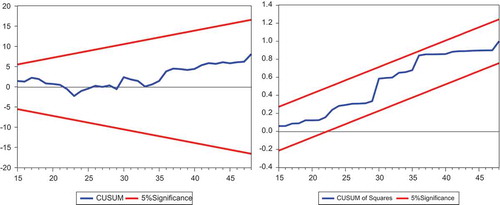
Finally, Figures 3 and 4 display tests for stability of the ARDL models using the CUSSUM and CUSSUM square techniques proposed by Brown, Durbin and Evans (1975). The result reveals that the models lie within the 5% significant level indicating that the null hypothesis that the models are stable cannot be rejected. Thus, the null hypothesis accepted that the models for the determinants of growth in government expenditure in Nigeria are stable at 5% level of significance.

Figure 3. Model 1 CUSSUM and CUSSUM square stability tests.

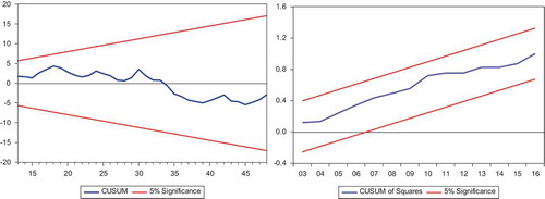
Figure 4. Model 2 CUSSUM and CUSSUM square stability tests.

Source: Computed by author using E-views 10.0.

6. Conclusion and policy recommendations

The study attempts to identify long-term determinants of government expenditure in Nigeria using time series data spanning between 1970 and 2017. The study slightly modified the Wagner’s law by incorporating other relevant variables that are assumed to be important in explaining the expansion of government expenditure in Nigeria. To achieve this objective, the paper applied autoregressive distributed lag (ARDL) model for data analysis.

The paper obtained variety of interesting results that are helpful for future policy prescription in government expenditure decision. The stationary properties of the time series data were checked. At level, only three variables were stationery. However, the remaining variables become stationery after taking their first difference which pave way for ARDL co-integration analysis. The bounds test revealed a long-run co-integration among the variables in the two models. The short-run and long-run results provide a strong support for Wagner’s. This implies that Wagner’s law holds for Nigeria indicating that the quest for industrialization and diversification has made government to embark on the provision of public infrastructures (railway, electricity and so on) which in turn causes expansion in public expenditure. The result also suggests that higher involvement of government in state activities has the capacity to push the size of public expenditure. To confirm the robustness of the results, we used more than one measures of government expenditure size and economic growth. Interestingly, all the models provided consistent results concerning the impact of income on government expenditure size.

Further, we find that inclusion of other control variables in the models provides fairly consistent results, suggesting that population, oil revenue, tax revenue, oil price and inflation are strong determinants of government expenditure size. Trade openness provides a mixed result in the two models. Other variables such as debt stock and exchange rate are found to have no significant effect on the share of government expenditure size. This might be due poor handling of debt contracted over the years especially during the decades of military regimes. Besides that, this may likely be explained through the fact that government may use the debt as a means to cover the revenue shortfall more than as a means of increasing spending, which means that the Nigerian government usually increases debt financing (budget deficit) whenever the revenue is short falling to maintain the existing spending. Based on the findings of the study, there is need for government to make a giant effort in diversifying the revenue base of the country to curtail the long-term effect of oil revenue fluctuation in the economy—since oil is the major source of revenue to the government and is exogenously determined by oil price in the international market. There is also need for proper use of debt in financing-efficient projects in the economy. This can be done by strengthening the anti-graft agencies so that they can be vigilant on the way and manner public debt is manage in the country. Given the strong positive correlation between population and government size, it is therefore important for government to encourage less family size through population reduction policies and legislations. This can be done to lessen the pressure of population explosion which is always accompanied by large demand of public utilities including education, health, pollution control, transfers, among others. To curtail the effect of price level on government expenditure decision, it is paramount for government to strengthening its monetary and fiscal policies towards ensuring stability in price level in the country.

Despite the promising results in this study, it is not free from certain limitations. First, the empirical analysis was conducted using aggregate data of government expenditure. An area of fruitful future research would be to analyse the data using disaggregate components of government expenditure. Such disaggregation will provide useful and robust findings for policy decisions. Second, the political aspect of the determinants of government expenditure is not captured in this study despite its significance in today’s context. Therefore, another useful extension of this study would be to consider including political variables.

Additional information

Funding

The authors received no direct funding for this research.

Notes on contributors

Adamu Jibir

Adamu Jibir is a lecturer in the Department of Economics, Gombe State University, Nigeria. He holds B.Sc. and Master’s degrees in Economics. Currently, he is a PhD scholar in the Department of Economics, University of Colombo, Sri Lanka. He has published in international peer-reviewed journals. His teaching and research interests include public economics, industrial organization, Islamic finance and small- and medium-scale enterprises.

Chandana Aluthge

Chandana Aluthge is a senior lecturer in Economics in the Department of Economics, University of Colombo, Sri Lanka. He holds PhD Degree in Economics from VU Amsterdam and MPhil from Maastrich University. He also obtained his M.A and B.A degrees in Economics from the University of Colombo, Sri Lanka. He has published in international peer-reviewed journals. His teaching and research interests encompasses monetary and fiscal policy operations, financial econometrics and research method.

References

- Abeng, M. O. (2005). Determinants of non-debt government expenditure in Nigeria. Central Bank of Nigeria Economic and Financial Review, 5(43), 43–23.
- Adamu, J., & Hajara, B. (2015). Government expenditure and economic growth nexus: Empirical evidence from Nigeria (1970–2012). IOSR Journal of Economics and Finance, 6(2), 61–69.
- Adamu, J., & Hajara, B. (2015). Impact of government expenditure and economic growth: Empirical evidence from Nigeria. IOSR Journal of Economics and Finance, 3(2), 61–68.
- Akanbi, O. A. (2014). Government expenditure in Nigeria: Determinants and trends. Mediterranean Journal of Social Sciences, 5(27), 98–115.
- Aladejare, S. A. (2019). Testing the robustness of public spending determinants on public spending decisions in Nigeria. International Economic Journal, 1–23.
- Ali, M. B., & Amin, A. (2018). Evaluation of revenue and expenditure hypotheses: Evidence from Pakistan (1972–2015). Economic and Social Review, 7(2), 65–77.
- Aregbeyen, O. O., & Akpan, U. F. (2013). Long-term determinants of government expenditure: A disaggregated analysis for Nigeria. Journal of Studies in Social Sciences, 5(1), 31–50.
- Athanasenas, A., Katrakilidis, C., & Trachanas, E. (2014). Government spending and revenues in the Greek economy: Evidence from non-linear co-integration. Empirica, 41(2), 365–376. doi:10.1007/s10663-013-9221-3
- Attari, M. I. J., & Javed, A. Y. (2013). Inflation, economic growth and government expenditure of Pakistan 1980–2010. Procedia Economic and Finance, 5, 58–67. doi:10.1016/S2212-5671(13)00010-5
- Aworinde, O. B. (2013). The tax-spend nexus in Nigeria: Evidence from nonlinear causality. Economics Bulletin, 33(4), 3117–3130.
- Bagdigen, M., & Cetintas, K. (2004). Causality between public expenditure and economic growth: The case of Turkey. Journal of Economic and Social Research, 6(1), 53–72.
- Baharumshah, A. Z., Jibrilla, A. A., Sirag, A., Ali, H. S., & Muhammad, I. M. (2016). Public revenue‐expenditure nexus in South Africa: Are there asymmetries? South African Journal of Economics, 84(4), 520–537. doi:10.1111/saje.2016.84.issue-4
- Baumol, W. J. (1967). Macroeconomics of unbalanced growth the anatomy of urban crisis. American Economic Review, 57(2), 415–426.
- Bird, R. M. (1971). Wagner’s law of expanding state activity. Public Finance, 26(1), 1–26.
- Blackley, P. R. (1986). Causality between revenues and expenditures and the size of the federal budget. Public Finance Review, 14(2), 139–156. doi:10.1177/109114218601400202
- Bolat, S. (2014). The relationship between government revenues and expenditures: Bootstrap panel granger causality analysis on European countries. Economic Research Guardian, 4(2), 2.
- Brown, C. V., & Jackson, P. M. (1994). Public sector economics (4th ed.). Oxford: Basil Blackwell.
- Brown, R. L., Durbin, J., & Evans, J. M. (1975). Techniques for testing the constancy of regression relationships over time. Journal of the Royal Statistical Society: Series B (Methodological), 37(2), 149–163.
- Cameron, D. R. (1978). The expansion of the public economy: A comparative analysis. The American Political Science Review, 72(4), 1243–1261. doi:10.2307/1954537
- CBN. (2017, December). Central bank of Nigeria statistical bulletin. Abuja.
- Dickey, D. A., & Fuller, W. A. (1981). Likelihood ratio statistics for autoregressive time series with a unit root. Econometrica: Journal of the Econometric Society, 49, 1057–1072. doi:10.2307/1912517
- Dizaji, S. F. (2014). The effects of oil shocks on government expenditures and government revenues nexus (with an application to Iran’s sanctions). Economic Modelling, 40, 299–313. doi:10.1016/j.econmod.2014.04.012
- Dreher, A. J., Strum, E., & Upsprung, H. (2008). The impact of globalization on the composition of government expenditures: Evidence from panel data. Public Choice, 134(3–4), 263–292. doi:10.1007/s11127-007-9223-4
- Durevall, D., & Henrekson, M. (2011). A futile quest for a grand explanation of long-run government expenditure. Journal of Public Economics, 95, 708–717. doi:10.1016/j.jpubeco.2011.02.004
- Epifani, P., & Gancia, G. (2009). Openness, government size and the term of trade. Review of Economic Studies, 76(2), 629–668. doi:10.1111/j.1467-937X.2009.00546.x
- Eterovic, D., & Eterovic, N. (2012). Political competition versus electoral participation: Effects on government’s size. Economics of Governance, 13(4), 333–363. doi:10.1007/s10101-012-0114-x
- Ezirim, B. C., Muoghalu, M. I., & Elike, U. (2008). Inflation versus public expenditure growth in the US: An empirical investigation. North American Journal of Finance and Banking Research, 2(2), 26–34.
- Facchini, F., & Melki, M. (2013). Efficient government size: France in the 20th century. European Journal of Political Economy, 31, 1–14. doi:10.1016/j.ejpoleco.2013.03.002
- Friedman, M. (1978). The limitations of tax. Policy Review, 5(78), 45–78.
- Gafar, J. (1975). The growth and structure of public expenditure and revenue in Guyana. Caribbean Studies, 15(3), 138–148.
- Goffman, I. J., & Mahar, D. J. (1971). The growth of public expenditure in selected developing nations: Six Caribbean countries (1940–65). Public Finance, 26(1), 58–75.
- Gupta, S. (1967). Public expenditure and economic growth: A time series analysis. Public Finance, 22(4), 423–461.
- Gyles, A. F. (1991). A time-domain transfer function model of Wagner’s law: The case of the United Kingdom economy. Applied Economics, 23, 327–330. doi:10.1080/00036849100000140
- Hayo, B. (1994). No further evidence of Wagner’s law for Mexico. Public Finance/Finances Publiques, 49, 287–294.
- Heller, P. S. (1975). A model of public fiscal behavior in developing countries: Aid, investment, and taxation. The American Economic Review, 2(2), 429-445.
- Henrekson, M. (1993). Wagner’s law - A spurious relationship? Public Finance, 48(3), 406–415.
- Jalles, J. (2019). Wagner’s law and governments’ functions: Granularity matters. Journal of Economic Studies, 46(2), 446–466. doi:10.1108/JES-02-2018-0049
- Jin, J., & Zou, H. F. (2002). How does fiscal decentralization affect aggregate, national, and subnational government size? Journal of Urban Economics, 52(2), 270–293. doi:10.1016/S0094-1190(02)00004-9
- Kesavarajah, M. (2012). Wagner’s law in Sri Lanka: An econometric analysis. International Scholarly Research Network, 7(1), 1–9.
- Kumar, S., Webber, D. J., & Fargher, S. (2012). Wagner’s Law revisited: Cointegration and causality tests for New Zealand. Applied Economics, 44(5), 607–616. doi:10.1080/00036846.2010.511994
- Lindblom, C. E. (1959). The science of muddling through. Public Administration Review, 19(Spring), 79–88. doi:10.2307/973677
- Magazzino, C., Giolli, L., & Mele, M. (2015). Wagner’s Law and Peacock and Wiseman’s displacement effect in European Union countries: A panel data study. International Journal of Economics and Financial Issues, 5(3), 812–819.
- Mann, A. J. (1980). Wagner’s law: An econometric tests for Mexico (1925–1976). National Tax Journal, 33(2), 189–201.
- Mauro, P. (1998). Corruption and the composition of government expenditure. Journal of Public Economics, 69(2), 263–279. doi:10.1016/S0047-2727(98)00025-5
- Michas, N. A. (1974). Application of covariance analysis to public expenditure studies. FinanzArchiv/Public Finance Analysis, 4(2), 295–304.
- Moalusi, D., (2004). Causal Link between government spending and revenue: A case study of Botswana (Fordham Economics Discussion Paper Series, Number dp2007–07).
- Mourao, P. R. (2007). Long-term determinants of Portuguese public expenditures. International Research Journal of Finance and Economics, 5(7), 45–67.
- Musgrave, R. (1966). Principles of budget determination. Public finance: Selected readings, 15-27.
- Musgrave, R. (1969). Principles of budget determination. In H. Cameroun & W. Henderson (Eds.), Public finance: Selected readings (pp. 56-69). New York: Random House.
- Mutascu, M. (2016). Government revenues and expenditures in the East European economies: A bootstrap panel granger causality approach. Eastern European Economics, 54(6), 489–502. doi:10.1080/00128775.2016.1204237
- Mutascu, M. (2017). The tax–Spending nexus: Evidence from Romania using wavelet analysis. Post-Communist Economies, 29(3), 431–447. doi:10.1080/14631377.2017.1319170
- Narayan, P. K., & Narayan, S. (2006). Government revenue and government expenditure nexus: Evidence from developing countries. Applied Economics, 38(3), 285–291. doi:10.1080/00036840500369209
- Njeru, J. (2003). The impact of foreign aid on public expenditure: The case of Kenya (AERC Working Paper, No. 23).
- Obeng, S. (2015). A causality test of the revenue-expenditure nexus in Ghana. ADRRI Journal of Arts and Social Sciences, 11(11), 1–19.
- Obeng, S. K., & Sakyi, D. (2017). Explaining the growth of public spending in Ghana. The Journal of Developing Areas, 51(1), 104–128. doi:10.1353/jda.2017.0006
- Ofori-Abebrese, G. (2012). A co-integration analysis of growth in government consumption expenditure in Ghana. Journal of African Development, 14(1), 12–23.
- Ogujiuba, K., & Abraham, T. W. (2012). Testing the relationship between government revenue and expenditure: Evidence from Nigeria. International Journal of Economics and Finance, 4(11), 172. doi:10.5539/ijef.v4n11p172
- Okafor, C., & Eiya, O. (2011). Determinants of growth in government expenditure: An empirical analysis of Nigeria. Research Journal of Business Management, 5(1), 44–50. doi:10.3923/rjbm.2011.44.50
- Olayungbo, D. O. (2013). Government spending and inflation in Nigeria: An asymmetry causality test. Growth, 10, 6.
- OPEC (2018). The Organization of Petroleum Exporting Countries Annual Statistical Bulletin.
- Parida, Y. (2012). Causal link between central government revenue and expenditure: Evidence for India. Economics Bulletin, 32(4), 2808–2816.
- Peacock, A. T., & Wiseman, J. (1961). The growth of public expenditure in the United Kingdom. London: Oxford University Press.
- Pelawaththage, N. K. (2019). An empirical investigation of Wagner’s law: The case of Sri Lanka (pp. 45-55). Colombo: Godage Publishers.
- Pesaran, H. M., & Shin, Y. (1995). Long-run structural modelling (No. 9419). Faculty of Economics, University of Cambridge, UK.
- Pesaran, M. H., Shin, Y., & Smith, R. J. (2001). Bounds testing to approaches to analysis of level relationships. Journal of Applied Econometrics, 16, 289–326. doi:10.1002/jae.616
- Pesaran, M. H., & Smith, R. (1997). Estimating long-run relationships from dynamic heterogeneous panels. Journal of Econometrics, 68(1), 79–113. doi:10.1016/0304-4076(94)01644-F
- Philips, P. B. C., & Perron, P. (1988). Testing for Unit Root in time series regression. Biometrica, 75, 335–346. doi:10.1093/biomet/75.2.335
- Phiri, A. (2016). Asymmetries in the revenue–Expenditure nexus: New evidence from South Africa. Empirical Economics, 5(1), 1–33.
- Pryor, F. L. (1968). Public expenditures in communist and capitalist nations. RD Irwin
- Richter, C., & Dimitrios, P. (2013). Tax and spend, spend and tax, fiscal synchronisation or institutional separation? Examining the case of Greece. Romanian Journal of Fiscal Policy, 4(2), 1.
- Richter, C., & Paparas, D. (2012). The validity of Wagner’s law in Greece during the last 2 centuries. INFER Working Paper, 2012(2), Bonn: International Network for Economic Research.
- Rodrik, D. (1998). Why do more open economies have bigger governments? Journal of Political Economy, 22(3), 295–352.
- Sagarik, D. (2014). Educational Expenditures in Thailand: Development, trends, and distribution. Citizenship, Social and Economic Education, 13(1), 53–66. doi:10.2304/csee.2014.13.1.54
- Sagdic, E. N., Sasmaz, M. U., & Tuncer, G. (2019). Wagner versus Keynes: Empirical evidence from Turkey’s provinces. Panoeconomicus, 1–18. doi:10.2298/PAN170531001S
- Saunoris, J. W. (2015). The dynamics of the revenue–expenditure nexus: Evidence from U.S. State government finances. Public Finance Review, 43(1), 108–134. doi:10.1177/1091142113515051
- Saunoris, J. W., & Payne, J. E. (2010). Tax more or spend less? Asymmetries in the UK revenue–Expenditure nexus. Journal of Policy Modeling, 32(4), 478–487. doi:10.1016/j.jpolmod.2010.05.012
- Shelton, C. A. (2007). The size and composition of government expenditure. Journal of Public Economics, 91, 2230–2260. doi:10.1016/j.jpubeco.2007.01.003
- Shonchoy, A. S. (2010). Determinants of government consumption expenditure in developing countries: A panel data analysis (Institute of Developing Economies (IDE) Discussion Paper, No. 266, Japan).
- Singh, B., & Sahni, B. S. (1984). Causality between public expenditure and national income. The Review of Economics and Statistics, 66, 630–644. doi:10.2307/1935987
- Taiwo, I. O. (1989). Determinants of federal government expenditure in Nigeria. Social and Economic Studies, 38(3), 205–222.
- Tang, T. C. (2006). Are imports and exports of OIC member countries co-integrated? A re-examination. Journal of Economics and Management, 14(1), 49–79.
- Thorn, R. S. (1972). The evolution of public finances during economic development (pp. 187-217). France: Rotterdam University Press.
- Uchenna, E., & Evans, O. (2014). Government expenditure in Nigeria: An examination of tri-theoretical mantras. Journal of Economic and Social Research, 14(2), 27–52.
- Ukwueze, E. R. (2015, October – December 1–8). Determinants of the size of public expenditure in Nigeria. Sage, doi:10.1177/2158244015621346
- Wagner, A. (1883). Finanzwissenschaft. Germany: Leipzig.
- WDI (2018). World Bank World Development Indicators.
- Wildavsky, A. B. (1964). The politics of the budgetary process. Boston: Little Brown.
- Zapf, M., & Payne, J. E. (2009). Asymmetric modelling of the revenue-expenditure nexus: Evidence from aggregate state and local government in the US. Applied Economics Letters, 16(9), 871–876. doi:10.1080/13504850701222095