Exchange rate and Chinese financial market: Variance decomposition under vector autoregression approach

Abstract

The foremost objective of the manuscript is to predict dynamic behaviour of economic and financial time series i.e. exchange rate and price of stock market in China and also to determine if there is a interrelation between the two. Monthly time series data of 10 years have been taken, from January 2009 to December 2018 (post-financial crisis of 2008). The unit root test, variance decomposition under vector autoregressive (VAR) approach, impulse response function and Granger causality under VAR environment have been smeared to infer the long and short-run statistical dynamics. The outcomes of vector autoregression approach depict that the two variables have positive impact and are statistically significant in the short run. There is no long-run association and causal relation between the exchange rate and Chinese financial market.

Keywords:

• vector autoregression
• China
• impulse response function
• stock market variance decomposition
• exchange rate
• VAR Granger causality

PUBLIC INTEREST STATEMENT

Financial markets are the main indicators to reveal the strength of the country’s economy. Then of course, there are some major economic determinants which lead to the fluctuation in the stock market up to a certain extent. The manner in which China’s money moves against the dollar could be the best proportion of how well US and Chinese exchange talks are continuing. To explore the dynamic behaviour of exchange rate of China to United States and its impact on the Chinese financial market is the prerequisite of present scenario. The significant ramifications of the investigation can be used by the government, individual and foreign investors and specialists of China for relevant policy formulation.

1. Introduction

China’s financial stoppage is beginning to burden a portion of the world’s greatest organizations. From Silicon Valley to Detroit, huge global organizations are feeling the impacts from the downturn on the planet’s second-biggest economy. Development in China a year ago was the weakest it has been in about three decades and the standpoint for 2019 could be more regrettable, as the exchange war with the United States keeps on harming the economy. It is very important to determine factors which have influence on the financial market of China.

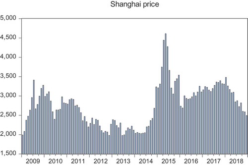
Figure 1. Graphical representation of stock market price of China.

Figure 1 represents the stock price volatility for Chinese market over the years. Y -axis represents thetime-period and X-axis represents the price.

Financial markets are the main indicators to reveal the strength of the country’s economy. Then of course, there are some major economic determinants which lead to the fluctuation in the stock market up to a certain extent. From a thorough study of several macroeconomic factors and how they have impact on financial markets, it is apparent that fluctuations in the market are basically affected by expansive cash supply, inflation credit/deposit proportion and monetary shortfall separated from political shakiness.

In this paper, we attempted to forecast the behaviour of exchange rate and Chinese financial market and also tried to evaluate the interrelation amid the two time series on a monthly data from 2009 to 2018 which is the post-financial crisis period using variance decomposition, Granger causality and impulse response function under vector autoregressive (VAR) approach.

The manner in which China’s money moves against the dollar could be the best proportion of how well US–Chinese exchange talks are continuing and to explore the dynamic behaviour of exchange rate of China to United States and its impact on the Chinese financial market is the prerequisite of the present scenario.

Explicitly, the core function of the study is to comprehend and predict the dynamic trend of exchange rate of China (USD/Yuan) and stock market price of China. Second, it is to identify the causative relationship between the two important variables of China under VAR model and also to determine if there is any interrelation or dependency between the two economic and financial series of China on short and long-run equilibriums.

The paper is organized in four different segments. The following area offers a short review of the related writing, trailed by the exchange of information and research technique in Section 3, while Section 4 introduces and talks about the fundamental experimental outcomes. At last, Section 5 closes with the exploration and conclusion.

2. Previous studies

Concentration on the share trading system and its effect on macroeconomic variables are not at the initial stage. It is continually being viewed as macroeconomic occasions that have a particular amount of stress on the securities exchanges. Liang and Teng (2006) demonstrated in his research the connection between financial and monetary development in China from 1952 to 2001. A multivariate VAR structure is utilized as a fitting detail and the relationship among budgetary improvement, expansion and additional significant growth factors was examined. The exact outcomes proposed that there is one way to lead–lag relation from monetary development to money-related improvement, which ends with drawing unmistakably from those in the past examinations. Shahbaz, Khan and Tahir (2013) examined the connection between energy use and monetary development by joining money-related improvement, universal exchange and capital as vital elements of creation work if there should be an occurrence in China in between 1971 and 2011. The latest technique ARDL, which limits testing to deal with integration, was connected to analyse the relationship in the long run among the arrangement, whereas stationarity properties were identified with the help of structural break test.

Uddin, Sjö and Shahbaz (2013) determined the connection between monetary progress and financial expansion in Kenya over time from 1971 to 2011. Since the monetary division assumes an essential part in assembling and apportioning funds into profitable endeavours, the main issue stays vital for creating financial matters. The research depends on a Cobb–Douglas generation increased by joining budgetary improvement. A re-enactment-based model ARDL limits testing in the study. Cointegration was identified between the arrangements within the sight of a basic break in 1992. Over the long haul, the advancement of the money-related segment positively affects monetary development. Chien, Lee, Hu and Hu (2015) looked at the vigorous procedure of union among securities exchanges in China and ASEAN-5 nations utilizing recursive integration investigation. The outcomes demonstrate that these six securities exchanges had at most one cointegrating vector in between 1994 and 2002. Generally speaking, the provincial monetary coordination among China and ASEAN-5 has been expanded step-by-step. Moreover, the evaluated coefficients of blunder redress terms are factually huge and adverse in China and Indonesia; however, the measurements of different nations are immaterial, implying that the majority of the alteration of this integration fell on these two nations’ securities exchanges.

Moore and Wang (2014) explored the origins of the vigorous connection between genuine trade rates and stock return discrepancies linking to the United States showcased in the markets of Asia. Initially, it was recognized as the dynamic provisional association of the two arrangements and later it was observed that the relation was deteriorated on the exchange balance and the loan fee differentials. Most of the time, the exchange balance is perceived to be a source element of the vibrant connection for some of the Asian countries, though the financing cost variance is the leading drive for some created markets. The latter gives the idea to reflect the high capital versatility. Granger, Huangb and Yang (2000) used unit root test and cointegration models to determine the causative associations between stock costs and trade rates utilizing ongoing Asian countries information. By means of drive reaction capacities (Impulse Response Functions), it is discovered that information from South Korea are in concurrence with the conventional methodology. That is, trade rates lead stock costs. Then again, information on the Philippines recommended the outcome expected under the portfolio methodology: stock costs lead trade rates with adverse affiliation. Evidence from Malaysia, Taiwan, Singapore, Hong Kong and Thailand demonstrate concrete input relations, while that of Indonesia and Japan neglect to uncover any unmistakable example.

Jayasuriya (2011) observed interlinkages of stock return conduct for China and three developing business sector neighbours from the Asia Pacific district from November 1993 to July 2008. Results depend on a VAR approach. Shocks or innovations (IR) and vector decay of VAR are additionally used. Proof recommends that the total markets are for the most part not interrelated. Be that as it may, relations among China and alternate markets when outside financial specialist returns are explicitly represented. Likewise, a stun beginning in China is altogether felt in the other value markets. Securities exchange qualities and macroeconomic states of these nations may encourage to clarify the spotted relations. Ono (2017) analysed the fund development interconnection in Russia with the vector autoregression demonstration, considering oil costs and outside trade rates. The broke down period is 1999–2008 and from 2009 to 2014. The outcomes for first time series recommend that there is causality from financial development to money supply and bank loaning, which infers request following reactions. The outcomes for other period demonstrate that financial development causes bank loaning while it was observed that there was no lead–lag relation from cash supply to monetary development.

Research by Büyüksalvarci and Abdioglu (2010) examined stock costs and its effect on macroeconomic factors on Turkey, the result of the examination encouraged that there is a unidirectional long-run connection between stock cost and macroeconomic factors.

The investigation of Kyereboah-Coleman and Agyire-Tettey (2008) uncovered that macroeconomic variables influence the execution of money markets in an unfavourable way. The outcome of the investigation suggested that just cash supply has a huge relationship with the Turkish Stock Index. Singh (2010) attempted to find a relationship among three macroeconomic variables and BSE Sensex by applying unit root tests, correlation and Granger causality test. The result of the investigation uncovered that the market list, exchange rate, Index of Industrial Production and discount value file were alienated.

Abu-Libdeh and Harasheh (2011) analysed causative connections of stock costs in Palestine with factors like gross domestic product, inflation rate, exchange rate, LIBOR and balance of trade and gathered quarterly information from the first Quarter of 2000 (March 2000) to the second Quarter of 2010 (June 2010). Regression signified to a noteworthy connection between every macroeconomic variable worried about stock costs of PEX (Palestine Exchange), while the causality investigation dismissed any sort of causal connections between all macroeconomic variable under examination and stock costs of PEX. Megaravalli and Sampagnaro (2018) perceived the connection among Indian, Chinese and Japanese securities exchanges and crucial macroeconomic factors, like, inflation and exchange rates. Month-to-month time sequence data in between January 2008 to November 2016 have been taken for the study. The results of pooled assessed consequences of ASIAN 3 nations demonstrate that the swapping scale has a positive and substantial long-run impact on securities exchanges while the inflation has an adverse and inconsequential long-run impact. Just round the corner, no factually noteworthy connection was observed between macroeconomic factors and securities exchanges. This examination accentuates on the effect of macroeconomic factors on the share trading system execution of a creating economy (India and China) and created economy (Japan).

3. Data and methodology

Monthly time series data from January 2009 to December 2018 are used in this study. Exchange rate and stock market price of China are the variables on which this research has been conducted. The data have been taken from the period of post-global financial crisis of 2008. Exchange rate of China to United States has been symbolized as USD_CHN and price of stock market from Shanghai stock exchange has been symbolized as SHANGHAI_PRICE. Data for both the variables have been taken from investing.com. Data have been taken for 10 years post-financial crisis period in order to know the influence of exchange rate and Chinese financial market after the global financial crisis.

The section further discusses the methods/models/techniques etc. which the study proposes to use on the data to extract the required information for the raw data.

3.1. Descriptive statistics

The study uses the data collected from various sources in its original form. The series is then subjected to initial analysis with the help of basic statistical tools before proceeding with econometric modelling. An underlying evaluation of mean and standard deviation of the arrangement is done to remark on the factors under investigation. Standard deviation is regularly utilized as a proportion of the risk related with value variances of a given resource. Standard deviation is a factual estimation that reveals insight into chronicled instability. The study of basic statistical measures has been coupled with the graphical study. Other factual measures under research are skewness and kurtosis. Skewness measure will enable us to comprehend the unevenness from the ordinary dissemination of the statistical data while Kurtosis processes the levelness of the dispersion of the series. Jarque–Bera test which is known as the goodness-of-fit test helps to confirm the condition of the normality of the data and also to check whether the data have the skewness and kurtosis even after being normally distributed. The formula to calculate this test is given in the following equation:

(1) $JB=\frac{n}{6}(S^2+\frac{1}{4}{\left(K-3\right)}^2$(1)

where JB is the Jarque–Bera, n is the number of observations, S is the skewness of data and K is the kurtosis of data.

In order to determine whether the data are normally distributed or not, JB measurement which has a chi-squared dispersion with two degrees of freedom has been used. The null hypothesis is a joint speculation of the skewness being 0 and the abundance kurtosis being 0. Tests from an ordinary dispersion have a normal skewness of 0 and a normal abundance kurtosis of 0 (which is equivalent to a kurtosis of 3). As the meaning of JB appears, any deviation from this expands the JB measurement and shows that the information isn’t normally distributed.

3.2. Test for stationary of data

After inferring whether the data are normally distributed or not, subsequently the investigation will continue to comprehend if the information under examination is stationary or not. A stationary procedure is the one whose joint possibility dispersion does not change when moved in time. Subsequently, the mean and variance, in the event that they are available, likewise don’t change after some time and don’t pursue any patterns.

A time series is stationary if it has the accompanying conditions:

• µ (mean) is constant for all t.

• σ (variance) is constant for all t.

• The autocovariance function between $X_{t_1}$ and $X_{t_2}$ only depends on the interval $t_1$ and $t_2$.

As it were, a stationary time arrangement ($X_t$) must have three highlights: finite variation, constant first moment and that the second moment just relies upon ($X_{t_1}$–$X_{t_2})$ and does not depend on $t_1$ and $t_2$.

The advanced econometrics portrays different tests to check for the stationery of the information. In any case, these tests have a few or the other downsides. Glynn, Perera and Verma (2007) have completed a broad survey of the ongoing advancements in the testing of the unit root theories within the sight of basic change and gave experimental proof.

The augmented Dickey–Fuller Test (1984) is an enhanced version of the first Dickey–Fuller Test (1979). The Dickey–Fuller test expressed that a basic autoregressive model (where the variable under examination is relapsed on its previous value) is demonstrated by

(2) $y_t=\alpha y_{t-1}+{\mu }_t$(2)

where y_t is the variable under study, t is the time index, α is the coefficient and µ_t is the error term.

In the event that α = 1, unit root is available in the information implying that the arrangement of the variable under investigation (it) is non-stationary for this situation. The Augmented Dickey-Fuller Test (ADF) test eliminates all the basic impacts (autocorrelation) in the time arrangement and afterwards tests utilizing a similar methodology. The testing technique for ADF is characterized in the following equation:

(3) $\mathrm{\Delta }{y}_t=\alpha +\beta t+\gamma y_{t-1}+\delta \mathrm{\Delta }{y}_{t-1}+\dots +{\delta }_{\rho -1}\mathrm{\Delta }{y}_{t-p+1}+{\epsilon }_t$(3)

where $\alpha$ is the constant, $\beta$ is the coefficient on a time trend and p is the lag order of the autoregressive process.

Forcing the requirements α = 0 and β = 0 relates to displaying an irregular walk and utilizing the limitation β = 0 compares to demonstrate an arbitrary stroll with a float. By comprising slags of the order p, the ADF definition takes into consideration higher arrange autoregressive procedures.

The hypotheses under examination while uses of the test are

$H_0$ = Series has a unit root.

$H_1$ = Series does not have a unit root.

If the value of t-statistics is found to be more than the critical value, then it implies that the null hypothesis will be rejected and it will be accepted in the case when the determined t-measurements are lower than the critical values. When the null hypothesis is found to be rejected as per the given condition, then data are observed to be non-stationary; in that case, first difference of the data has to be determined. The first difference of the time series is nothing but the change between the time period that is between t and t − 1. In other words,

(4) $\mathrm{\Delta }{Y}_t=Y_t-Y_{t-1}$(4)

The difference of the series will be calculated until it becomes stationary.

3.3. Vector autoregression model

The VAR demonstration is utilized to decide the relationship among a few factors. You can utilize a VAR for anticipating, as we did with the ARIMA and GARCH models; however, as we found with those, the conjectures are typically not sufficiently exact to be such useful from a reasonable viewpoint. Rather, by and by, the analyst will more often than not finish up taking a gander at the accompanying three things that are gotten from the fitted VAR demonstrate: Granger causality, impulse response functions and variance decomposition, that uncover something about the idea of how these variables move together. System equation or model developed for vector autoregression for this particular research.

The two models with two dependant variables are

$\begin{array}{rl}& \mathbf{D}\left(\mathbf{U}\mathbf{S}\mathbf{D}\mathrm{\_}\mathbf{C}\mathbf{H}\mathbf{N}\right)=\mathbf{C}\left(\mathbf{1}\right)\ast \mathbf{D}\left(\mathbf{U}\mathbf{S}\mathbf{D}\mathrm{\_}\mathbf{C}\mathbf{H}\mathbf{N}\left(-\mathbf{1}\right)\right)+\mathbf{C}\left(\mathbf{2}\right)\ast \mathbf{D}\left(\mathbf{U}\mathbf{S}\mathbf{D}\mathrm{\_}\mathbf{C}\mathbf{H}\mathbf{N}\left(-\mathbf{2}\right)\right)+\\ & \mathbf{C}\left(\mathbf{3}\right)\ast \mathbf{D}\left(\mathbf{S}\mathbf{H}\mathbf{A}\mathbf{N}\mathbf{G}\mathbf{H}\mathbf{A}\mathbf{I}\mathrm{\_}\mathbf{P}\mathbf{R}\mathbf{I}\mathbf{C}\mathbf{E}\left(-\mathbf{1}\right)\right)+\mathbf{C}\left(\mathbf{4}\right)\ast \mathbf{D}\left(\mathbf{S}\mathbf{H}\mathbf{A}\mathbf{N}\mathbf{G}\mathbf{H}\mathbf{A}\mathbf{I}\mathrm{\_}\mathbf{P}\mathbf{R}\mathbf{I}\mathbf{C}\mathbf{E}\left(-\mathbf{2}\right)\right)+\mathbf{C}\left(\mathbf{5}\right)\end{array}$

$\begin{array}{rl}& \mathbf{D}\left(\mathbf{S}\mathbf{H}\mathbf{A}\mathbf{N}\mathbf{G}\mathbf{H}\mathbf{A}\mathbf{I}\mathrm{\_}\mathbf{P}\mathbf{R}\mathbf{I}\mathbf{C}\mathbf{E}\right)=\mathbf{C}\left(\mathbf{6}\right)\ast \mathbf{D}\left(\mathbf{U}\mathbf{S}\mathbf{D}\mathrm{\_}\mathbf{C}\mathbf{H}\mathbf{N}\left(-\mathbf{1}\right)\right)+\mathbf{C}\left(\mathbf{7}\right)\ast \mathbf{D}\left(\mathbf{U}\mathbf{S}\mathbf{D}\mathrm{\_}\mathbf{C}\mathbf{H}\mathbf{N}\left(-\mathbf{2}\right)\right)+\\ & \mathbf{C}\left(\mathbf{8}\right)\ast \mathbf{D}\left(\mathbf{S}\mathbf{H}\mathbf{A}\mathbf{N}\mathbf{G}\mathbf{H}\mathbf{A}\mathbf{I}\mathrm{\_}\mathbf{P}\mathbf{R}\mathbf{I}\mathbf{C}\mathbf{E}\left(-\mathbf{1}\right)\right)+\mathbf{C}\left(\mathbf{9}\right)\ast \mathbf{D}\left(\mathbf{S}\mathbf{H}\mathbf{A}\mathbf{N}\mathbf{G}\mathbf{H}\mathbf{A}\mathbf{I}\mathrm{\_}\mathbf{P}\mathbf{R}\mathbf{I}\mathbf{C}\mathbf{E}\left(-\mathbf{2}\right)\right)+\mathbf{C}\left(\mathbf{10}\right)\end{array}$

Since in such a model all factors rely upon one another, singular parameter esteems just give constrained data. So as to show signs of improvement instinct of the model’s powerful conduct, drive reactions (IR) are utilized. They give the response of a reaction variable to a one-time stun in a motivation variable. The direction of the reaction variable can be plotted, which results in those wavy bends that can be found in numerous large-scale papers.

4. Empirical findings

Table 1 characterizes the framework of descriptive statistics of both the variables i.e. exchange rate symbolizes with USD_CHN and the Shanghai stock exchange market price of China symbolizes with Shanghai price. Before engaging in any kind of regression analysis, it is essential to have information contained in the data set. With the help of this table, we can get the information regarding the measures of central tendency through the values of mean, median and mode and also get the information of measures of dispersion from the values of variance and standard deviation that is how far the deviations are from the sample average. We can also obtain the information of measures of normality from kurtosis which measures the sharpness of the distribution of the series and from skewness which measures the degree of asymmetry of the series. As per the values of kurtosis and skewness, it can be determined that both the time series are normally distributed as the value of kurtosis of stock market price is around 3 and the skewness value is around 0, and if the value of kurtosis of exchange rate is lower than 3, it signifies the flatted curve. Jarque–Bera test statistic measures the difference of the skewness and kurtosis of the series with those from the normal distribution. Probability is associated with the Jarque–Bera test statistics which accept that the null hypothesis denotes that data are not normally distributed for both the variables. Therefore, descriptive statistic gives the clear picture about the data set.

Table 1. Descriptive statistics

Descriptive statistics
	SHANGHAI PRICE	USD CHN
Mean	2,765.852	6.496821
Median	2,770.755	6.469150
Maximum	4,611.740	6.975600
Minimum	1,979.210	6.054000
Std. dev.	532.4736	0.273197
Skewness	0.636827	0.107356
Kurtosis	3.681932	1.562282
Jarque–Bera	10.43613	10.56568
Probability	0.005418	0.005078
Sum	331,902.2	779.6185
Sum sq. dev.	33,739,847	8.881747
Observations	120	120

*Note: Descriptive statistics of the variables used in the study.

Source for Data—Investing.com and analysis done on Eviews.

Moving on to the graphical representation of both the variables, In Figure 1, we can see that stock market price of China is not normally distributed. It keeps fluctuating with the time, though following the same trend for years but fell down and remained same for 2012–2014. Alternatively, the price increased very high in 2015 and then decreased and follows the same pattern from 2016 to 2017 and then tends towards falling down in 2018.

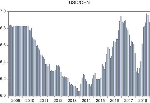
Looking at Figure 2, very high volatility and fluctuations specifically can be observed from 2010 onwards and keeps decreasing till 2013 and then moving upwards and keeps fluctuating which clearly depicts that data set is not normally distributed.

Figure 2. Graphical representation of exchange rate of China.

Figure 2 depicted high volatility and fluctuations in the exchange rate of China over the years.

These actualities are additionally settled by the ADF test, which is an appropriate and legitimate testing system for deciding the stationary or non-stationary nature of the information outline.

The ADF measurements appeared in Table 2 uncover that both the variables of China observed to be non-stationary in levels, with block and slacked 0. Each variable of China observed to be non-stationary on the grounds that they neglected to dismiss the invalid speculation i.e. the null hypothesis, which demonstrates variable, has the nearness of unit root which implies that variables are not stationary at level.

Table 2. Unit root test (at level)

ADF unit root test (at level)
	Variables	t-statistic	p-value*	Result
	SHANGHAI_PRICE	−2.752055	0.0685	(not stationary)
	USD_CHN	−1.682634	0.4374	(not stationary)

Note: The null hypothesis is rejected if test statistic > critical value. Critical value considered at 5% significant value. * 5% significance level.

Table 3 represents the consequence of the ADF test in the wake of taking the first difference. The resultant estimation of the ADF test insights is contrasted and basic qualities for the above factors. Every one of the factors after taking the first difference to the time arrangement observed to be stationary. Subsequently, in the wake of utilizing ADF test, presently VAR model, impulse response function, variance decomposition and Granger causality test under VAR environment have been applied further to test the long-haul combination between the financial and economic factors of China.

Table 3. Unit root test (at first difference)

ADF unit root test (at first difference)
Variables	t-Statistic	p-value*	Result
SHANGHAI_PRICE	−8.004826	0.0000	(stationary)
USD_CHN	−7.612424	0.0000	(stationary)

Note: A null hypothesis is accepted if test statistic < critical value. Critical value considered at 5% significant level. * 5% significance level.

After examining whether the data are stationary or not, the optimal lag length has to be identified. On the basis of AIC criteria, the maximum lag length identified is 2. Table 4 represents the estimates of vector autoregression model. There are two equations with two dependant variable. One dependant variable is exchange rate of China and another dependant variable is stock market price of China and the independent variables are their two lags. In Table 4, we can see the results of VAR model.

Table 4. Vector auto regressive estimates

Vector autoregression estimates
Standard errors in () and t-statistics in []
	D(USD_CHN)	D(SHANGHAI_PRICE)
D(USD_CHN(−1))	0.345612	−434.7233
	(0.09663)	(351.673)
	[3.57649]	[−1.23616]
D(USD_CHN(−2))	−0.003268	177.5774
	(0.09707)	(353.258)
	[−0.03367]	[0.50268]
D(SHANGHAI_PRICE(−1))	2.83E − 05	0.158242
	(2.6E − 05)	(0.09434)
	[1.09125]	[1.67736]
D(SHANGHAI_PRICE(−2))	−7.44E − 07	−0.116652
	(2.6E − 05)	(0.09443)
	[−0.02869]	[−1.23537]
C	−8.60E − 05	1.194185
	(0.00528)	(19.2008)
	[−0.01630]	[0.06219]

Note: Estimate the vector error regression model.

The two models with two dependant variables are

$\begin{array}{rl}& \mathbf{D}\left(\mathbf{U}\mathbf{S}\mathbf{D}\mathrm{\_}\mathbf{C}\mathbf{H}\mathbf{N}\right)=\mathbf{C}\left(\mathbf{1}\right)\ast \mathbf{D}\left(\mathbf{U}\mathbf{S}\mathbf{D}\mathrm{\_}\mathbf{C}\mathbf{H}\mathbf{N}\left(-\mathbf{1}\right)\right)+\mathbf{C}\left(\mathbf{2}\right)\ast \mathbf{D}\left(\mathbf{U}\mathbf{S}\mathbf{D}\mathrm{\_}\mathbf{C}\mathbf{H}\mathbf{N}\left(-\mathbf{2}\right)\right)+\\ & \mathbf{C}\left(\mathbf{3}\right)\ast \mathbf{D}\left(\mathbf{S}\mathbf{H}\mathbf{A}\mathbf{N}\mathbf{G}\mathbf{H}\mathbf{A}\mathbf{I}\mathrm{\_}\mathbf{P}\mathbf{R}\mathbf{I}\mathbf{C}\mathbf{E}\left(-\mathbf{1}\right)\right)+\mathbf{C}\left(\mathbf{4}\right)\ast \mathbf{D}\left(\mathbf{S}\mathbf{H}\mathbf{A}\mathbf{N}\mathbf{G}\mathbf{H}\mathbf{A}\mathbf{I}\mathrm{\_}\mathbf{P}\mathbf{R}\mathbf{I}\mathbf{C}\mathbf{E}\left(-\mathbf{2}\right)\right)+\mathbf{C}\end{array}$

$\begin{array}{rl}& \mathbf{D}\left(\mathbf{S}\mathbf{H}\mathbf{A}\mathbf{N}\mathbf{G}\mathbf{H}\mathbf{A}\mathbf{I}\mathrm{\_}\mathbf{P}\mathbf{R}\mathbf{I}\mathbf{C}\mathbf{E}\right)=\mathbf{C}\left(\mathbf{6}\right)\ast \mathbf{D}\left(\mathbf{U}\mathbf{S}\mathbf{D}\mathrm{\_}\mathbf{C}\mathbf{H}\mathbf{N}\left(-\mathbf{1}\right)\right)+\mathbf{C}\left(\mathbf{7}\right)\ast \mathbf{D}\left(\mathbf{U}\mathbf{S}\mathbf{D}\mathrm{\_}\mathbf{C}\mathbf{H}\mathbf{N}\left(-\mathbf{2}\right)\right)+\\ & \mathbf{C}\left(\mathbf{8}\right)\ast \mathbf{D}\left(\mathbf{S}\mathbf{H}\mathbf{A}\mathbf{N}\mathbf{G}\mathbf{H}\mathbf{A}\mathbf{I}\mathrm{\_}\mathbf{P}\mathbf{R}\mathbf{I}\mathbf{C}\mathbf{E}\left(-\mathbf{1}\right)\right)+\mathbf{C}\left(\mathbf{9}\right)\ast \mathbf{D}\left(\mathbf{S}\mathbf{H}\mathbf{A}\mathbf{N}\mathbf{G}\mathbf{H}\mathbf{A}\mathbf{I}\mathrm{\_}\mathbf{P}\mathbf{R}\mathbf{I}\mathbf{C}\mathbf{E}\left(-\mathbf{2}\right)\right)+\mathbf{C}\left(\mathbf{10}\right)\end{array}$

We have developed VAR model with two dependant variables. In the whole system equation, there are 10 coefficients. We can see in the first equation that coefficient ends with C(5) and in the next equation, it starts with C(6) which implies that this is a system equation model which is linked with each other. Now to check whether the USD_CHN lag 1 and lag 2 are significant to explain Shanghai price, we have to look for Table 5 which is system equation table. To check this, we can check the associated p-value of that coefficient if the p-value is less than 0.05, then it is significant, else not. Therefore, USD_CHN lag 1 and lag 2 are not significant to explain Shanghai price. In this way, all the variables can be checked whether they are significant or not.

Table 5. VAR: system equation

Estimation method: least squares
	Coefficient	Std. error	t-Statistic	p-value
C(1)	0.345612	0.09663	3.576488	0.0004*
C(2)	−0.00327	0.09707	−0.03367	0.9732
C(3)	2.83E − 05	2.59E − 05	1.09125	0.2763
C(4)	−7.44E − 07	2.59E − 05	−0.02869	0.9771
C(5)	−8.60E − 05	0.00528	−0.0163	0.987
C(6)	−434.723	351.673	−1.23616	0.2177
C(7)	177.5774	353.258	0.502684	0.6157
C(8)	0.158242	0.09434	1.677363	0.0949
C(9)	−0.11665	0.09443	−1.23537	0.218
C(10)	1.194185	19.2008	0.062195	0.9505

*Indicates the significant level at 5%.

In this system equation, only USD_CHN lag1 is significant to explain USD_CHN because its p-value is less than 5%.

Figure 3 shows the results of impulse response function under VAR. We can see different graphs with response of one to standard deviation shock to the other. Blue line is impulsive response function line while the red lines are simply the 95% coefficient intervals. The impulse response function always lies within 95% coefficient interval. We can observe the response or the reaction of one to the other. In the first graph, we can observe the response of USD_CHN to simply deviation shock to USD_CHN which is called own shock. It is observed that one SD own shock initially decreases in periods 1 and 2, then it slightly increases in periods 3 and 4 and then becomes stable. In the second graph, we observed the response of exchange rate to the stock market price. A one SD shock or innovation of exchange rate to stock price initially has noticeable impact on stock market price, it increases from 1 to 2 period and then gradually decreases being in the positive zone and then becomes stable. Thus, shocks to exchange rate will have impact on stock market price in the short run.

Figure 3. Results of impulsive response function.

Figure 3 represents the impulsive reaction of the variables.

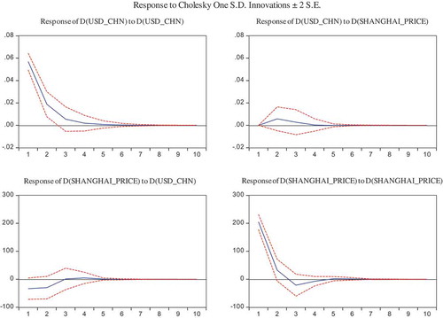
In the third graph, a shock on stock market price has impact on the exchange rate as it tends to increase gradually and moves towards positive from negative and becomes steady at zero. There is interrelation between the two in the short run.

The fourth graph demonstrated sharp decline from positive to negative, an then gradually tends towards increment and becomes stable, thus we can see the noticeable impact of own shock of stock market price.

In Tables 6 and 7, we can see the results of variance decomposition under VAR environment with two variables. All the variables are stationary at first difference because VAR model needs stationary data to run it. Lag selection criterion that is AIC criteria has advised us to take 2 lags in the VAR model to be optimum lags and then we have developed VAR followed by variance decomposition with two endogenous variables. The result of variance decomposition of variable 1 that is exchange rate of China (Table 6) period denotes the 10-year period as we have taken monthly data of 10 years. With this, we can predict the future also as projections usually inferred from the past trends. There are two things short run and long run, if we consider 3rd period, it is short run and if we consider 10th year, then it is known as long run. In the short run, impulse or innovation or shock to exchange rate accounts for 98.88% variation of the fluctuation in exchange rate that is termed own shock. In the second shock, a shock to stock market price can cause or influence 1.14% fluctuation in exchange rate and for the long run also condition is the same which depicts that there is short-run equilibrium between the two. There is impact but the degree of impact is low between the two variables. For own shock impact is high.

Table 6. Variance decomposition of USD_CHN

Variance decomposition of D(USD_CHN)
Period	SE	D(USD_CHN)	D(SHANGHAI_PRICE)
1	0.056278	100.0000	0.000000
2	0.059498	99.06066	0.939343
3	0.059824	98.85388	1.146122
4	0.059854	98.82680	1.173199
5	0.059856	98.82402	1.175978
6	0.059857	98.82377	1.176226
7	0.059857	98.82375	1.176246
8	0.059857	98.82375	1.176248
9	0.059857	98.82375	1.176248
10	0.059857	98.82375	1.176248

Note: Describe the variable decomposition of the exchange rate of China against dollar.

Table 7. Results of variance decomposition of Shanghai price

Variance decomposition of D(SHANGHAI_PRICE)
Period	SE	D(USD_CHN)	D(SHANGHAI_PRICE)
1	208.3112	2.609306	97.39069
2	212.0319	4.180340	95.81966
3	212.3349	4.447555	95.55245
4	212.3709	4.478142	95.52186
5	212.3748	4.481038	95.51896
6	212.3751	4.481283	95.51872
7	212.3752	4.481302	95.51870
8	212.3752	4.481303	95.51870
9	212.3752	4.481303	95.51870
10	212.3752	4.481303	95.51870

Note: Describe the variable decomposition of the price of the financial market of China (Shanghai price).

Likewise, it has been observed from the results of variance decomposition of Shanghai price from Table 7 that if we consider third year, it would be considered as short run. Thus, in the short run, shock to exchange rate accounts for 4.44% variation of the fluctuation in the stock market price of China and shock to Shanghai price can contribute 95.5% fluctuation in the variation of Shanghai price. Therefore, there is impact of 4.44% to the stock market price in the short run and same in the long run.

Table 8 demonstrates the results of VAR Granger causality test. We have observed that exchange rate is the dependent variable and stock market price is the independent variable. Null hypothesis depicts that stock market price of China does not lead or cause exchange rate of China. When we observed the p-value, as p-value is greater than 5% at 5% significance level, we cannot reject the null hypothesis which stated that Shanghai price doesn’t lead or cause exchange market of China.

Table 8. Results of VAR Granger causality test

VAR Granger causality/block exogeneity Wald tests
Sample: 2009M01 2018M12
Dependent variable: D(USD_CHN)
Excluded	Chi-sq.	df	p-value
D(SHANGHAI_PRICE)	1.242732	1	0.2649
All	1.242732	1	0.2649
Dependent variable: D(SHANGHAI_PRICE)
Excluded	Chi-sq.	df	p-value
D(USD_CHN)	1.456190	1	0.2275
All	1.456190	1	0.2275

Estimations are done using Eviews software. Monthly data from 2009 to 2018.

When the dependent variable is stock market price and the independent variable is the exchange rate of China then, the null hypothesis is that exchange rate of China does not lead or cause Shanghai price. When we observe the p-value, it is greater than 5% by which we cannot reject the null hypothesis. Therefore, it can be inferred that exchange rate of China doesn’t lead or cause stock market price of China. Therefore, there is no causal or lead–lag relationship between the two.

5. Conclusion

The research has endeavoured towards the assessment of the dynamic behaviour of the exchange rate and stock market price and their interrelation with each other for the post-global financial crisis period using VAR model, variance decomposition, impulse response function and Granger causality under VAR approach in the short run or long run. In the present globalized period, where capital markets are winding up altogether incorporated, it has turned out to be basic to comprehend the basic essentials affecting the business sectors at residential and worldwide dimension.

The vector autoregression approach indicated that there is short-run association of exchange rate and stock market price of China. Impulse response function and variance decomposition under VAR indicated that there is a positive relation between the two variables and they are statistically significant in the short run. The degree of association between the two in the long run is very low. There is no long-run integration between the two. And my results are supported by Megaravalli and Sampagnaro (2018) that there is no long run cointegration between the exchange rate and stock market price in their research work. VAR Granger causality examines that there is no lead–lag or causal relation between the two.

The present investigation has further extension for exhaustive outcomes. It tends to reach out over a more drawn out period and with a few nations and by comprising different macroeconomic factors, it will be further fascinating to perceive the way, stock exchange is influenced by macroeconomic factors in European, United States and other created showcase. Imminent investigation can likewise concentrate on near investigation of creating and created markets. The significant ramifications of the investigation can be to administrations of China for the individual and institutional financial specialists for the policy makers and foreign investors.

Additional information

Funding

The authors received no direct funding for this research.

Notes on contributors

Shweta Ahalawat

Shweta Ahalawat is a post-doctoral student at the Indian Institute of Management Rohtak. She has completed her doctoral studies in Management from Banasthali Vidyapith. She was a member of Research team at IIM Udaipur and IIM Rohtak. Her research interest includes financial markets, derivatives and macroeconomic variables.

References

- Abu-Libdeh, H., & Harasheh, M. (2011). Testing for correlation and causality relationships between stock prices and macroeconomic variables. The case of Palestine Securities Exchange. International Review of Business Research Papers, 7(5), 141–154.
- Büyüksalvarci, A., & Abdioglu, H. (2010). The causal relationship between stock prices and macroeconomic variables: A case study for Turkey. International Journal of Economic Perspectives, 4(4), 601.
- Chien, M. S., Lee, C. C., Hu, T. C., & Hu, H. T. (2015). Dynamic Asian stock market convergence: Evidence from dynamic cointegration analysis among China and ASEAN-5. Economic Modelling, 51, 84–14. doi:10.1016/j.econmod.2015.06.024
- Glynn, J., Perera, N., & Verma, R. (2007). Unit root tests and structural breaks: A survey with applications.
- Granger, C. W., Huangb, B. N., & Yang, C. W. (2000). A bivariate causality between stock prices and exchange rates: Evidence from recent Asianflu☆. The Quarterly Review of Economics and Finance, 40(3), 337–354. doi:10.1016/S1062-9769(00)00042-9
- Jayasuriya, S. A. (2011). Stock market correlations between China and its emerging market neighbors. Emerging Markets Review, 12(4), 418–431. doi:10.1016/j.ememar.2011.06.005
- Kyereboah-Coleman, A., & Agyire-Tettey, K. F. (2008). Impact of macroeconomic indicators on stock market performance: The case of the Ghana stock exchange. The Journal of Risk Finance, 9(4), 365–378. doi:10.1108/15265940810895025
- Liang, Q., & Jian-Zhou, T. (2006). Financial development and economic growth: Evidence from China. China Economic Review, 17(4), 395–411.
- Megaravalli, A. V., & Sampagnaro, G. (2018). Macroeconomic indicators and their impact on stock markets in ASIAN 3: A pooled mean group approach. Cogent Economics & Finance, 6(1), 1432450. doi:10.1080/23322039.2018.1432450
- Moore, T., & Wang, P. (2014). Dynamic linkage between real exchange rates and stock prices: Evidence from developed and emerging Asian markets. International Review of Economics & Finance, 29, 1–11. doi:10.1016/j.iref.2013.02.004
- Ono, S. (2017). Financial development and economic growth nexus in Russia. Russian Journal of Economics, 3(3), 321–332. doi:10.1016/j.ruje.2017.09.006
- Shahbaz, M., Khan, S., & Tahir, M. I. (2013). The dynamic links between energy consumption, economic growth, financial development and trade in China: Fresh evidence from multivariate framework analysis. Energy Economics, 40, 8–21. doi:10.1016/j.eneco.2013.06.006
- Singh, D. (2010). Causal relationship between macro-economic variables and stock market: A case study for India. Pakistan Journal of Social Sciences (PJSS), 30, 2.
- Uddin, G. S., Sjö, B., & Shahbaz, M. (2013). The causal nexus between financial development and economic growth in Kenya. Economic Modelling, 35, 701–707. doi:10.1016/j.econmod.2013.08.031