Exploring the drivers of tracking error constrained portfolio performance

Abstract

Maximising returns is often the primary goal of asset management but managing and mitigating portfolio risk also plays a significant role. Successful active investing requires outperformance of a benchmark through skillful stock selection and market timing, but these bets necessarily give rise to risk. The risk, relative to the benchmark, is the tracking error and active managers are constrained by investment mandates including a restriction on tracking error. The locus of possible portfolio risks and returns, constrained by a tracking error is elliptical, and the main axis slope’s sign and magnitude varies under different market conditions. How these variations affect portfolio performance is explored for the first time. We find that changes in main axis slope (magnitude and sign) acts as an early indicator of portfolio performance and could therefore be used as another risk management tool.

Keywords:

• maximum diversification
• tracking error frontier
• main axis slope
• portfolio optimisation

JEL CLASSFICATION:

• C51
• D81
• G11
• G23

PUBLIC INTEREST STATEMENT

Profitable investing is traditionally assessed via high returns, but skilful asset management involves generating these returns above a suitable benchmark while simultaneously managing the portfolio’s risk. Successfully accomplishing these dual objectives is increasingly difficult in the current (2019) environment of sustained low-interest rates, elevated market volatility and global trade uncertainty. These complexities mean fund managers must increasingly relying on complex mathematical tools to achieve their aims. Tools such as the tracking error and its associated frontier are examples of such formulations which, used correctly, can provide insight into profitable asset allocation. Portfolio risk is constrained by the tracking error frontier. The universe of acceptable investable securities (and combinations thereof) is governed by this metric, but the behaviour and role of these frontiers in portfolio performance has been largely neglected. This work expands upon other recent studies and explores the market drivers which govern the frontier’s behaviour. The output of this investigation offers a valuable addition to fund manager experience and broad economic knowledge.

1. Introduction

Investment styles are broadly classified as passive or active. For the former, fund managers purchase and hold securities (or fractions of market indices) for extended investment periods believing that market outperformance is impossible, so best to minimise transactions (and hence fees) and be satisfied with returns like the broad market. For the latter, managers assume that through skilful selection and timing of sales and purchases, market outperformance is possible. The emphasis in the latter investment style is on relative performance, so skill (outperformance) is assessed relative to a prescribed, mandated benchmark. Risk is also assessed relative to the benchmark’s risk.

Markowitz’s efficient frontier (1956) formulation has directed passive investment research for almost seven decades and the literature on associated portfolio optimisation is considerable. Sharpe (1964) introduced the concept of a maximum risk-adjusted return portfolio for “optimal” performance, called the tangent portfolio (Jansen and van Dijk, 2002). Active investment strategies involve more complex structures, because here constraints restrict the investable universe. Benchmark constituents, the size of tracking error (portfolio risk relative to the benchmark) and asset weight floors and caps all contribute to additional complexity (Ammann and Zimmermann, 2001). Roll (1992) initiated research into tracking error (TE) constrained portfolio behaviour and developed the framework for describing an efficient frontier in risk/return space constrained by various levels of TE. Jorion (2003) extended this work and developed the details for the constant TE frontier: i.e. a locus of points in risk/return space which embraces the universe of risk/return combinations—relative to the benchmark’s risk and return.

TE is an active risk measure (defined as the standard deviation of the difference between portfolio and benchmark returns) that reflects a portfolio manager’s decisions to deviate from the weights of a benchmark’s positions with the aim of outperforming the benchmark. The inevitable risk introduced by this deviation is the TE. The TE is generally not used as a risk metric to assess portfolio manager performance in isolation (Clarke, de Silva, and Thorley, 2002). Rather, other measures are used in combination with the TE to assess portfolio risk, such as Value at Risk, the information ratio, etc. Fund managers determine the investment policy (i.e. its risk-return profile, outperformance targets, etc.) which in turn determines the TE. Thomas, Rottschafer, and Zvingelis (2013) outline several causes of TE (fees, transaction costs, taxes, factor tilts, cash management and market volatility).

In mean/variance space, the universe of possible portfolios constrained by a TE is an ellipse (and in risk/return space, it is a distorted ellipse). The ellipse’s orientation (designated by the sign and magnitude of the “main axis” slope) changes through time as economic conditions change. The way the main axis slope changes under different economic conditions, is explored here for South African (SA) stocks (an emerging third world economy) for the first time. We outline the relevant mathematics required to calculate both the sign and magnitude of the main axis slope and we evaluate the way this slope changes as time evolves and market conditions change. We find that when the main axis slope changes sign sharply, this presages a prolonged downturn in economic conditions. The effect is subtle, however. Forecasting economic conditions (and hence investment strategy) may depend on slope sign changes, but this depends on the direction of the change (i.e. $+ve$ to $-ve$), the magnitude of the slope before the reversal and the speed and size of the reversal. The combinations are persistent and robustly predict near economic conditions with reasonable accuracy. We thus find that the way the main axis slope moves through time could trigger novel investment strategies for active fund managers.

The remainder of this article proceeds as follows: A literature review is provided in Section 2 which gives insight to the relevant contextual background to the various investment strategies available. Thereafter, the available literature regarding the discovery of the mean/variance framework, which ultimately lead to Jorion’s (2003) finding of the constant tracking error (TE) frontier, is reviewed. Section 3 provides a discussion of the data selection as well as the underlying relevant mathematics governing the choice of asset weights within an emerging economy (SA). This section also provides the mathematics to the construction of the constituents which comprise Figure 1. Section 4 illustrates the results of the analysis and discusses the results obtained. Section 5 concludes the article and provides investment enhancing recommendations.

Figure 1. Positions of relevant frontiers and portfolios in the risk/return plane.

Source: Author calculations.

2. Literature review

Markowitz (1952) formulated the mean/variance framework which indicated to investors their coordinates in a return/risk plane. An efficient set of portfolios (i.e. those with a maximum return at a given absolute risk level) trace out a hyperbolic curve in this return/risk space. Sharpe (1964) established the maximum risk-adjusted portfolio return—now known as the Sharpe ratio. This ratio measures the quotient of excess return (over the risk-free rate) and portfolio risk (defined by its volatility) given as

$SR=\frac{{\mu }_P-r_f}{{\sigma }_P}.$

where ${\mu }_P$ is the portfolio annual return, $r_f$ is the annualised risk-free rate and ${\sigma }_P$ is the portfolio-annualised volatility (or risk).

Two investment styles dominate the market: passive management (known as buy-and-hold, which is generally cheaper) and active management (strategic stock selection and timing, generally more expensive). Both passive and active fund managers are evaluated and remunerated depending on their propensity to outperform the broad market. The former accomplishes this by taking and holding small bets relative to market indices, whilst the latter attempts to generate outperformance of a prescribed benchmark (usually a market index or a—sometimes arbitrary—combination of securities) by taking a combination of bets and timing market movements. Active managers are often also constrained by a TE, which may not be exceeded under the mandated investment contract (Daly and van Vuuren, 2019).

Passive fund managers generally aim for the maximum Sharpe ratio (tangent) portfolio on the efficient frontier (Markowitz, 1952) although there are several other possibilities in which passive fund managers may explore, such as the minimum variance portfolio (for highly risk-averse investors), the maximum diversification (Theron and van Vuuren, 2018) or minimum intra-correlation portfolios (for risk-averse investors), etc (Wu and Jakshoj, 2011). Active manager performance is evaluated using several criteria, one of which is the TE (Jorion, 1992).

Roll (1992) set out the description of the maximum return portfolio, relative to a benchmark, for a given TE, a formulation that describes a hyperbolic curve, much like the efficient frontier (but shifted to the right—i.e. riskier), in risk-return space. Absolute portfolio risk is neglected in Roll’s (1992) approach, so these portfolios are not optimal in a mean-variance sense and they are always riskier than the benchmark. The problem of mean-variance maximisation under a TE constraint was reconsidered by Bertrand, Prigent, and Sobotka (2001) who reintroduced both absolute and relative risk (i.e. TE) aversion into their optimisation program. A range of optimisation and holding periods while ignoring transaction cost constraints was considered by Larsen and Resnick (2001). Frequent rebalancing was necessary to maintain control over total risk (though not TE risk) when portfolios are actively managed (see also Plaxco & Arnott, 2002), but this did not always lead to optimal portfolios (El-Hassan & Kofman, 2003). Jorion (2003) tackled these and other problems and established the shape of the constant TE portfolio, an ellipse in the traditional mean-variance plane, but not in mean/risk plane (where it is a distorted ellipse with no bi-axial symmetry).

When TE could vary and risk aversion was fixed (rather than only considering constant TE frontier-constrained portfolios) Bertrand (2009) found that the resulting optimal portfolios exhibited many desirable properties, such as having the same information ratio. The IR decomposition proposed by Menchero and Hu (2006) was also explored evaluated by Bertrand (2010) using risk-adjusted performance attribution previously developed by Bertrand (2005).

The literature was largely silent on absolute portfolio risk in the active management arena, until work by Maxwell, Daly, Thomson, and van Vuuren (2018) unveiled a way to determine the asset weights to construct the TE-constrained tangent portfolio—effectively the maximum Sharpe ratio (tangent) portfolio on the constant TE frontier. This approach produced portfolios with a lower risk, but greater return than the agent’s benchmark whilst satisfying the TE constraint and maximising the Sharpe ratio (Riccetti, 2010).

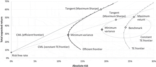
The efficient frontier is shown in Figure 1 as well as the minimum variance and tangent portfolios (the latter at the intersection of the capital market line (CML) and the efficient frontier (in this example, $r_f=7\mathrm{\%}$)). The riskier TE frontier appears to the right of the efficient frontier: this is the locus of coordinates on the risk/return plane with the highest return at increasing values of TE relative to a benchmark (Evans and van Vuuren, 2019). Where $TE=0\mathrm{\%}$, the TE frontier necessarily intersects the benchmark. Finally, also shown in Figure 1 is the distorted ellipse of the constant TE frontier (here, $TE=6\mathrm{\%}$), with the minimum variance, maximum Sharpe and maximum return portfolios. The tangent portfolio is at the intersection of the constant TE frontier and its CML (Maxwell et al., 2018). The maximum return portfolio on the constant TE frontier is the maximum return coordinate on the constant TE frontier for every value of TE (Stowe, 2014). Note the slightly positive slope of the constant TE frontier ellipse in this configuration (Maxwell and van Vuuren, 2019).

The main axis slope, $S_{MA}$ (defined as the slope of the line joining the efficient frontier’s minimum variance portfolio and the benchmark portfolio) and its relationship with TE-constrained portfolio performance is investigated here for the first time.

3. Data and methodology

3.1. Data

South Africa is an emerging economy with a history of political scandals and a volatile currency. The data for both benchmark and portfolios comprised 20 assets from the Johannesburg Stock Exchange (JSE) selected from a variety of market sectors to diversify the portfolio. The portfolio spans at least seven market sectors and seven of the largest, most liquid stocks are shown in Table 1. These assets are frequently traded by active managers. Monthly returns spanning 15 years from Oct-00 to Apr-19 were used. This era embraces various market conditions: the years of expansionary conditions which preceded the 2007–9 credit crisis, the credit crisis and post-credit crisis turmoil.

Table 1. Top seven stocks (by liquidity and market capitalisation) details

	Description	Sector
Naspers	A global internet and entertainment group and one of the largest global technology investors	Media
AVI	Active in the food market sector and embraces a range of categories including hot beverages, biscuits and snacks, frozen convenience foods, personal care products, cosmetics	Food producers
Shoprite	Africa’s largest food retailer	Food and drug retailers
Remgro	An investment holding company with interests in banking, financial services, packaging, glass products, medical services, mining, petroleum, beverage, food and personal care products.	Financial services
MTN	Telecommunications network provider offering mobile communications, internet data bundles and mobile contracts.	Mobile telecomms
ARM	Niche, diversified South African mining company with long-life, low-cost operating assets in key ARM mines and beneficiates iron ore, manganese ore, chrome ore, platinum group metals, copper, nickel and coal	Industrial metals and mining
Sappi	Leading global provider of sustainable wood fibre products and solutions	Forestry & Paper

Source: Bloomberg.

The benchmark was rebalanced monthly and comprised equal proportions of these highly liquid shares. The descriptive statistics of these securities are set out in Table 2.

Table 2. Descriptive statistics

	Naspers	AVI	Shoprite	Remgro	MTN	ARM	Sappi
Mean annual return	32.40%	20.97%	22.21%	17.99%	11.08%	20.25%	10.36%
Max monthly return	40.18%	20.27%	22.35%	19.76%	31.49%	42.77%	27.23%
Min monthly return	−48.57%	−18.45%	−16.38%	−12.18%	−28.09%	−31.89%	−43.33%
Cumulative 19y return	5 217%	2 056%	2 181%	1 495%	182%	613%	114%
Annualised volatility	22.07%	20.39%	25.80%	17.47%	26.34%	39.54%	24.54%
Skewness	−0.672	0.072	0.123	0.142	0.158	0.283	−0.275
Kurtosis	4.690	0.110	−0.142	0.833	1.152	1.060	1.822

Source: Bloomberg and authors’ calculations.

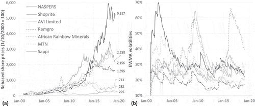
Figure 2(a) illustrates all stocks’ rebased cumulative share prices (rebased on Oct-00 = 100) and Figure 2(b) shows the exponentially weighted moving average (EWMA) volatilities of the stocks.

Figure 2. (a) Rebased cumulative share prices (Oct-00 = 100) and (b) exponentially weighted moving average (EWMA) volatilities of constituent stocks.

Source: Bloomberg and authors’ calculations.

3.2. Methodology

Active fund managers are assessed based on outperformance of a specified benchmark. The active investment positions they take differ from the benchmark positions according to the mandate governing the fund. For low TEs, active weights are small. For higher TEs, active weights are larger reflecting the fact that bigger bets are possible. Higher TEs, then, permit a wider range of security weights to be taken advantage of, rewarding skilled fund managers with potentially higher returns than the benchmark. The underlying variables, matrices and matrix notation, are defined below for a sample of $N$ component securities:

$\mathit{q}$:      $1\times N$ vector of benchmark weights

$\mathit{x}$:      $1\times N$ vector of deviations from the benchmark

${\mathit{q}}_{\mathit{P}}\left(=q+x\right)$: $1\times N$ vector of portfolio weights

$\mathit{E}$:      $1\times N$ vector of expected returns,

$\mathit{\sigma }$:      $1\times N$ vector of benchmark component volatilities

$\mathit{\rho }$:      $N\times N$ benchmark correlation matrix

$\mathit{V}$:      $N\times N$ covariance matrix of asset returns

$\mathbf{1}:1\times N$ vector of 1s and

$r_f$:      the risk-free rate.

Net short sales are allowed so the total active weights ($q_i+x_i$) may be $<0$ for individual securities. The universe of assets may be larger than the benchmark’s component set, but for Roll’s (1992) methodology, no assets outside the benchmark’s set may be included. Expected returns and variances are expressed in matrix notation as:

${\mu }_B=\mathit{q}E\prime$:   expected benchmark return

${\sigma }_B=\sqrt{\mathit{q}V{q}^{\prime }}$: volatility (risk) of benchmark return

${\mu }_{\epsilon }=\mathit{x}E\prime$:   expected excess return; and

${\sigma }_{\epsilon }=\sqrt{\mathit{x}V{\mathit{x}}^{\prime }}$:  TE.

The active portfolio expected return and variance is given by ${\mu }_P=\left(\mathit{q}+x\right)\mathit{E}\prime ={\mu }_B+{\mu }_{\epsilon }$ and ${\sigma }_P=\sqrt{\left(\mathit{q}+x\right)\mathit{V}\left(\mathit{q}+x\right)\prime }$ respectively. The portfolio must be fully invested, so $\left(\mathit{q}+x\right)\mathbf{1}\prime =1$.

Merton (1972) defined $a=\mathit{E}{\mathit{V}}^{-1}\mathit{E}\prime ,b=\mathit{E}{\mathit{V}}^{-1}1\prime ,c=\mathbf{1}{\mathit{V}}^{-1}\mathbf{1}\prime ,d=a-\frac{b^2}{c}$ and ${\mathrm{\Delta }}_1={\mu }_B-\frac{b}{c}$ where $b/c={\mu }_{MV}$ and ${\mathrm{\Delta }}_2={\sigma }_B^2-\frac{1}{c}$ with $1/c={\sigma }_{MV}^2$ where $MV$is the minimum variance portfolio.

It is useful to recall the mathematics required to generate the various frontiers.

3.2.1. Mean variance frontier

Minimise ${\mathit{q}}_P\mathit{V}{q}_P^{\prime }$ subject to ${\mathit{q}}_P\mathbf{1}\prime =1$ and ${\mathit{q}}_P\mathit{E}\prime =G$ where $G$ is the target return. The vector of portfolio weights is ${\mathit{q}}_P=\left(\frac{a-bG}{d}\right)q_{MV}+\left(\frac{bG-\frac{b^2}{c}}{d}\right){\mathit{q}}_{\mathit{T}G}$ where ${\mathit{q}}_{\mathit{M}V}$ is the vector of asset weights for the minimum variance portfolio given by ${\mathit{q}}_{\mathit{M}V}={\mathit{V}}^{-1}\frac{1}{c}$ and ${\mathit{q}}_{\mathit{T}G}$ is the vector of asset weights for the tangent portfolio (with $r_f=0)$, i.e. ${\mathit{q}}_{\mathit{T}G}={\mathit{V}}^{-1}\frac{\mathit{E}}{b}$. The weights of the tangent portfolio’s components, ${\mathit{q}}_{\mathit{T}P}$, with $r_f\ne 0$, are:

${\mathit{q}}_{\mathit{T}P}^{\prime }=\frac{{\mathit{V}}^{-1}\left(\mathit{E}-r_f\cdot \mathbf{1}\right)\prime }{\mathbf{1}\cdot {\mathit{V}}^{-1}\left(\mathit{E}-r_f\cdot \mathbf{1}\right)\prime }$

3.2.2. TE frontier

Maximise $\mathit{x}E\prime$ subject to $\mathit{x}1\prime =0$ and $\mathit{x}Vx\prime ={\sigma }_{\epsilon }^2$. The solution for the vector of deviations from the benchmark is $\mathit{x}\prime =\pm \sqrt{\frac{{\sigma }_{\epsilon }^2}{d}}{\mathit{V}}^{-1}{\left(\mathit{E}-\frac{b}{c}\mathbf{1}\right)}^{\prime }$. The solution to this optimisation problem generates the TE frontier, a portfolio’s maximal return at a given risk level and subject to a TE constraint. The benchmark may be efficient, in which case it would lie on the efficient frontier. The benchmark is often rather arbitrarily selected (a mix of stock and bonds or an imperfect market index) so it frequently is not a member of the efficient portfolio set. The TE frontier passes through the benchmark coordinates when here $TE=0$.

3.2.3. Constant TE frontier

Maximise $\mathit{x}E\prime$ subject to $\mathit{x}\mathbf{1}\prime =0$, $\mathit{x}Vx\prime ={\sigma }_{\epsilon }^2$ and $\left(\mathit{q}+x\right)\mathit{V}\left(\mathit{q}+x\right)\prime ={\sigma }_P^2$. The vector of deviation weights from the benchmark is $\mathit{x}\prime =-\frac{1}{{\lambda }_2+{\lambda }_3}{\mathit{V}}^{-1}\left(\mathit{E}\prime +{\lambda }_1+{\lambda }_3\mathit{V}q\prime \right)$ where ${\lambda }_1=-\frac{{\lambda }_3+b}{c}$, ${\lambda }_2=\pm \left(-2\right)\sqrt{\frac{d{\mathrm{\Delta }}_2-{\mathrm{\Delta }}_1^2}{4{\sigma }_{\epsilon }^2{\mathrm{\Delta }}_2-y^2}}-{\lambda }_3$ and ${\lambda }_3=-\frac{{\mathrm{\Delta }}_1}{{\mathrm{\Delta }}_2}\pm \frac{y}{{\mathrm{\Delta }}_2}\sqrt{\frac{d{\mathrm{\Delta }}_2-{\mathrm{\Delta }}_1^2}{4{\sigma }_{\epsilon }^2{\mathrm{\Delta }}_2-y^2}}$. The solution for this optimisation describes an ellipse—a constant TE frontier—in return/risk space: the unconstrained constant TE frontier (Jorion, 2003). The north-west segment of this frontier is bounded on the west by the minimum variance portfolio (with ${\sigma }_P=\sqrt{\left({\sigma }_B^2+TE+2\sqrt{TE\cdot \left({\sigma }_B^2-{\sigma }_{MV}^2\right)}\right)}$) and in the north by the maximum return portfolio (with deviations from the benchmark weights given by $\mathit{x}\prime =\pm \sqrt{\frac{{\sigma }_{\epsilon }^2}{d}}{\mathit{V}}^{-1}{\left(\mathit{E}-\frac{b}{c}\mathbf{1}\right)}^{\prime }$). The arc between these portfolios on the unconstrained constant TE frontier represents the efficient set of portfolios subject to a specific TE. The solution for the weights which generate the tangent portfolio (to the constant TE frontier) was recently found by Maxwell et al. (2018) to involve solving for ${\sigma }_P$ using:

$\frac{\left(r_f-{\mu }_B\right)}{{\sigma }_P^2}+\frac{\frac{\left({\mathrm{\Delta }}_1^2-d{\mathrm{\Delta }}_2\right)\cdot \left({\sigma }_P^2-{\sigma }_B^2-{\sigma }_{\epsilon }^2\right)}{\sqrt{\left({\mathrm{\Delta }}_1^2-d{\mathrm{\Delta }}_2\right)\left[{\left({\sigma }_P^2-{\sigma }_B^2-{\sigma }_{\epsilon }^2\right)}^2-4{\mathrm{\Delta }}_2{\sigma }_{\epsilon }^2\right]}}+{\mathrm{\Delta }}_1}{{\mathrm{\Delta }}_2}-\frac{\sqrt{\left({\mathrm{\Delta }}_1^2-d{\mathrm{\Delta }}_2\right)\left[{\left({\sigma }_P^2-{\sigma }_B^2-{\sigma }_{\epsilon }^2\right)}^2-4{\mathrm{\Delta }}_2{\sigma }_{\epsilon }^2\right]}+{\mathrm{\Delta }}_1\cdot \left({\sigma }_P^2-{\sigma }_B^2-{\sigma }_{\epsilon }^2\right)}{2{\mathrm{\Delta }}_2{\sigma }_P^2}$

then, establishing ${\mu }_P$ on the efficient segment of the constant TE frontier and then backing out the relevant weights (see Figure 1).

3.2.4. Main axis slope, S_MA

The main axis slope, $S_{MA}$ is calculated using

(1) $S_{MA}=\frac{{\mathrm{\Delta }}_1}{{\sigma }_B-{\sigma }_{MV}}=\frac{{\mu }_B-\frac{b}{c}}{{\sigma }_B-{\sigma }_{MV}}=\frac{{\mu }_B-{\mu }_{MV}}{{\sigma }_B-{\sigma }_{MV}}$(1)

${\mathrm{\Delta }}_1$ determines the sign of $S_{MA}$ because the denominator is always $>0$ since ${\sigma }_B-{\sigma }_{MV}>0$ always. A necessary and sufficient condition for $S_{MA}<0$ is ${\mu }_B<{\mu }_{MV}$. Note that the $S_{MA}$ is independent of TE since none of its components depend explicitly thereon. We measure and evaluate, for the first time, the sign and magnitude of the $S_{MA}$ and we explore how these (and constituents of the $S_{MA}$) change over time as market conditions evolve plus their influence on TE-constrained portfolio performance.

Figure 3 shows the relevant frontiers, portfolios and the long axis—calculated using (1). The periods are (a) Sep-10 when $S_{MA}<0$ and (b) Apr-11 when $S_{MA}>0$.

Figure 3. Efficient, TE and constant TE frontiers and the main axis for (a) Sep-10 (${\mathit{S}}_{\mathit{M}A}=-\mathbf{2.64}\mathbf{[}<\mathbf{0}\mathbf{]}$) and (b) Apr-11 (${\mathit{S}}_{\mathit{M}A}=+\mathbf{2.82}[>\mathbf{0}]$). $\mathit{T}E=\mathbf{6}\mathrm{\%}$ and ${\mathit{r}}_f$ was the annualised 3-month SA treasury rate. Different levels of TE were used but generated very similar results.

Source: Bloomberg and authors’ calculations.

4. Results and discussion

Figure 4 shows the regression results of the $S_{MA}$ versus the tangent portfolio’s Sharpe ratios (the latter shown in Figure 1). We compare and regress against this particular portfolio—the maximum Sharpe ratio portfolio—because we assert that most active managers will aim for this rather than the maximum return portfolio (Roll, 1992), the portfolio with the same risk as the benchmark (Jorion, 2003) or the minimum variance portfolio on the constant TE frontier. The tangent portfolio is the optimal portfolio subject to a given TE constraint, so it lies on the efficient portfolio set, has a higher return than that of the benchmark and frequently (but not always) has a lower risk than the benchmark. Although the tangent portfolio does not generate the maximum return, it maximises the risk-adjusted return for a given TE (Maxwell et al., 2018).

Figure 4. ${\mathit{S}}_{\mathit{M}A}$ regressed on the tangent portfolio’s maximum Sharpe ratios.

Source: Authors’ calculations.

An $R^2=0.41$ indicates a positive relationship between $S_{MA}$ and the maximum Sharpe ratios of the tangent portfolio. This relationship is expected: an $S_{MA}>0$ requires that ${\mu }_B>{\mu }_{MV}$. Higher Sharpe ratios require higher risk-adjusted returns, hence the positive relationship between maximum Sharpe ratios and the $S_{MA}$.

Splitting the dataset into two and regressing the metrics over two time periods, (a) Nov-05 to Oct-12 and (b) Nov-12 to Apr-19 shows that these changed over time from being highly correlated to ($\rho =0.88$) to only marginally correlated ($\rho =0.46$)—see Figure 5. This is more clearly shown in Figure 7.

Figure 5. ${\mathit{S}}_{\mathit{M}A}$ regressed on the tangent portfolio’s maximum Sharpe ratios for the period (a) Nov-05 to Oct-12 and (b) Nov-12 to Apr-19.

Source: Authors’ calculations.

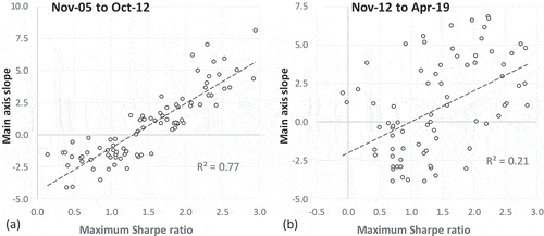
The start of 2013—the point at which the relationship between the $S_{MA}$ and the maximum Sharpe ratio deteriorates—saw significant economic upheaval in South Africa. South Africa was downgraded in early 2013 by one major credit rating agency (SA National Treasury, 2013) and later that year by another (Moody’s, 2013). The market became more volatile and the earnings of several corporates with international holdings became more volatile because of inevitable currency fluctuations. The consequences of this are discussed later.

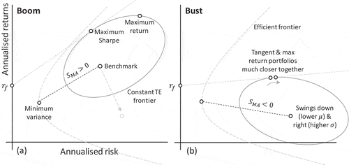
Why the $S_{MA}$ and the Sharpe ratio would be correlated is better explained using Figure 6 for two economic milieus, (a) boom: $S_{MA}>0$ and (b) bust: $S_{MA}<0$. Figure 5(a) sets out the stylised, relative positions of frontiers and portfolios under boom conditions. Figure 6(b) shows the stylised position, in risk/return space, of these frontiers and portfolios in a downturn period.

In this configuration, Figure 6(a) shows an $S_{MA}>0$ because ${\mathrm{\Delta }}_1>0$. The efficient frontier comprises portfolios with long and short positions and is relatively stable,¹ as is the minimum variance portfolio (known to be considerably less volatile than the benchmark—see Figure 9) so these positions are similar in the two periods. The benchmark—being more volatile than the minimum variance portfolio—suffers a decrease in returns and an increase in risk, so it shifts down and right in the risk/return plane. In sufficiently severe downturns, this can mean $S_{MA}<0$ and the coordinates of the tangent and maximum return portfolios move much closer together, i.e. their risk and return profiles become almost indistinguishable. Because the risk of the maximum Sharpe ratio portfolio increases in market downturns and its return decreases, there should be a strong relationship between the $S_{MA}$ and the maximum Sharpe ratio (as observed).

Figure 6. Stylised, relative positions of frontiers and portfolios under (a) boom and (b) bust conditions. As a direct result, when ${\mathit{S}}_{\mathit{M}A}<\mathbf{0}$, the tangent portfolio Sharpe ratio is likely to be low, as observed (Figure 7).

Source: Authors.

The relationship between $S_{MA}$ and the maximum Sharpe ratio from the tangent portfolio over time is shown in Figure 7.

Figure 7. The tangent portfolio’s Sharpe ratio and the ${\mathit{S}}_{\mathit{M}A}$: the grey dashed line indicates the time of multiple credit rating agency downgrades. Circles indicate turning points and the grey-shaded area indicates a developing trend in which the two series diverge considerably.

Source: Authors’ calculations.

The Sharpe ratio and the $S_{MA}$ evolve similarly, but some interesting features are worth elucidating—particularly those which may be used to trigger investment decisions. The point at which the positive relationship deteriorates is early 2013, indicated by the grey-dashed line (see Figure 5). In this strongly correlated phase (Figure 5(a)) the onset of the 2008 financial crisis marks the beginning of a sustained decline for both series (explained in Figure 6). The grey circles which occur when $S_{MA}>0$ and are proceeded by a substantial decrease in both quantities (the $S_{MA}$ changing from $+8$ to $-4$ and the maximum Sharpe decreasing by $\approx 60\mathrm{\%}$ over a few months in both cases). The grey circles indicating turning points when $S_{MA}<0$ are proceeded by an increase in both quantities (but considerably less for the $S_{MA}$ compared with changes when $S_{MA}>0$ and the maximum Sharpe increasing by $\approx 80\mathrm{\%}$ again over a few months).

In the less correlated phase (Figure 5(b)) the situation is less clear. Sharp turning points when the $S_{MA}>0$ result in corresponding small ($\approx 20\mathrm{\%}$) changes in the maximum Sharpe ratio. Sharp changes in $S_{MA}$ when it is $<0$ sometimes results in large changes in the maximum Sharpe ratio (e.g. mid 2013, $\approx 120\mathrm{\%}$) and sometimes not (e.g. $\approx 10\mathrm{\%}$ in early 2014). The significant changes in the $S_{MA}$ both decreasing and increasing in early 2016 had almost no effect on the maximum Sharpe value.

Since Feb-18, the close relationship between $S_{MA}$ and the maximum Sharpe ratio measured has diverged even more (grey-shaded region in Figure 7). South Africa’s first technical recession in 9 years was announced in Q2-18 which increased market risk and lowered annual returns (Figure 7). The combination of these effects contributed to the lowest measured Sharpe ratios in the entire 15-year observation period. During the same time, the $S_{MA}$ remained positive (if only slightly) and has only begun to increase more recently. It is possible that the benchmark, comprising large, liquid stocks, has not experienced the substantial losses (and increase in risk) as those in the maximum Sharpe ratio portfolio. As a result, $S_{MA}$ has remained positive, while the maximum Sharpe ratio has continued to decline.

These results could be used to signal exit and entry strategies in the tangent portfolio. Sharp reversals in the sign of $S_{MA}$ indicate a prolonged period of poor performance if $S_{MA}$ changes rapidly from $>0$ to $<0$ in boom conditions. The reverse is also true, $S_{MA}$ sign reversals indicate a prolonged period of superior performance if $S_{MA}$ changes rapidly from $<0$ to $>0$, again, in boom conditions. Large changes in the magnitude of $S_{MA}$ lead directly to large changes in the maximum Sharpe ratio, and hence performance of the tangent portfolio.

Figure 8 shows the excess returns (over $r_f$) and portfolio volatility for the maximum Sharpe ratio portfolio. Note that these are the constituents of the Sharpe ratio calculation.

Figure 8. Components of the maximum Sharpe ratio portfolio (numerator: excess return (over ${\mathit{r}}_f=\mathbf{6}\mathrm{\%}$) and denominator: ${\sigma }_{\mathit{P}}$, calculated over the same observation period for comparison). The combination of lower returns and higher risk recently (shaded area) has contributed to the decline in the maximum Sharpe ratio over the same period (shaded area in Figure 7).

Source: Author calculations.

Figure 9 shows the $S_{MA}$ and the annualised returns of the minimum variance and benchmark portfolios (averaged over three years). Note the relative volatility of returns for the two portfolios’ returns.

Figure 9. Annualised returns of the benchmark and minimum variance portfolio (averaged over three years) and the ${\mathit{S}}_{\mathit{M}A}$ over the same observation period for comparison.

Source: Author calculations.

To demonstrate the correlation between the returns of the maximum Sharpe ratio and those of the benchmark, the returns were regressed on each other and a high $R^2=0.92$ was found. It is not surprising that the returns of these portfolios should move together; they comprise the same constituents and the tracking error is tight ($TE=6\mathrm{\%}$), so portfolio managers will be discouraged from taking bets far from the benchmark weights. The regression (Figure 10) shows that by investing in the tangent portfolio, returns can be expected to be $\approx 10\mathrm{\%}$ greater than those generated from the benchmark portfolio—for all levels of ${\mu }_B$, even 0%. This reflects a highly desirable information ratio of 1.67 (relative return over the benchmark 10%, from a relative risk $TE=6\mathrm{\%}$).

Figure 10. Regression of (a) monthly maximum Sharpe ratio portfolio returns and (b) monthly minimum variance portfolio returns on monthly benchmark portfolio returns.

Source: Author calculations.

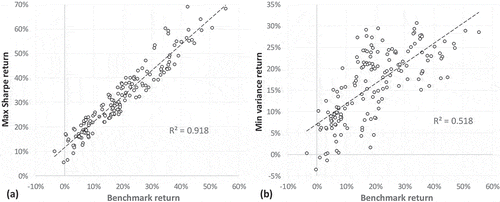
Although a positive correlation still exists between the returns of the minimum variance portfolio and those of the benchmark, the latter influences the former considerably less ($R^2$ here $=0.52$). It has already been shown that they the returns of these portfolios—although positively correlated—have substantially different volatilities (see Figure 9) with ${\sigma }_{MV}<{\sigma }_B$. The minimum variance portfolio generates returns which are invariably greater (by $\approx 7\mathrm{\%}$) than those of the benchmark which leads to $S_{MA}>0$ more often than $S_{MA}<0$ (54.7% versus 45.3%).

The weights in the respective stocks as a function of time is shown in Figure 11. Three major incidents are identified: credit ratings downgrades, corruption scandals and the “Nenegate” affair. These give rise to notable, dramatic changes in the evolving profile of security weights as well as the sharp changes in $S_{MA}$ shown in Figure 7.

Figure 11. Relative portfolio constituent weights (${\mathit{x}}_i$) for the maximum Sharpe ratio portfolio on the constant TE frontier over the observation period. Recall that $\sum _i{x}_i=0$.

Source: Bloomberg and authors’ calculations.

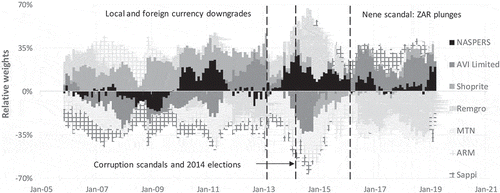
Prior to the 2013 local and foreign currency downgrade by Fitch ratings, relative holdings in Naspers fluctuates between overweight and underweight the benchmark. However, after the announcement of the downgrade (and after the 2014 corruption scandals, the uncertainty regarding the May 2014 elections and the Nenegate affair of November 2015) relative holdings in Naspers become positive and remain consistently overweight to the benchmark. Note that with monthly rebalancing note that this implies continuous increases of the weightings in Naspers. Naspers invests internationally and thus an investment in Naspers reflects considerable diversification benefits. When the ZAR depreciates it is beneficial to invest in a company which has international holdings.

Although MTN experienced good performance up until their $5.2 billion fine in 2015 it was optimal to underweight the stock relative to the benchmark weights as its performance was not as stellar as Naspers and Shoprite. Naspers and Remgro both have international holdings whereas Shoprite, MTN and African Rainbow Minerals are companies whose activities are predominantly in the developing market space. During political uncertainty and associated devaluation of the ZAR, it is crucial to overweight the companies with international holdings and consecutively underweight shares whose activities are predominantly based in the emerging market space. This reiterates the importance of foreign diversification.

Naspers as well as AVI Limited’s relative weightings increase significantly after Sept-18. This is due to both stocks consisting of international holdings and this period proceeds the announcement of South Africa’s first technical recession in 9 years (Sep-18). Again, this highlights the importance of international diversification.

5. Conclusion and recommendations

South Africa is an emerging economy which experiences periods of financial turmoil, political scandals and considerable currency fluctuations. Following these periods of turmoil, large rebalancing of relative asset weights is required (Figure 11). The results and findings reiterate the importance of diversification, for any developing economy, especially in stocks which contain a percentage of international holdings. Investors, however, shy away from uncertainty and constant rebalancing because of the high transaction costs and tax liabilities: foreign investments have decreased in South Africa over the recent past.

The significant positive relationship between the $S_{MA}$ and the maximum Sharpe ratio confirms the link between these metrics and the possibility of a trading strategy. During boom conditions, sharp $S_{MA}$turning points when $S_{MA}\ge 0$ trigger roughly 12 months of improving or deteriorating Sharpe ratios, depending on whether the turning point was a local maximum or minimum. Investors may adjust portfolio holdings accordingly. In bust conditions, when the market experiences currency weakness, high market volatility or both, the $S_{MA}$is an unreliable indicator or future market moves and should not be used. These result, and possible investor actions, are summarised in Table 3.

Table 3. Investment strategies from sharp turning points in $S_{MA}$

	Boom	Bust
$S_{MA}>0$, downturn	Sell portfolio or decrease holdings. $\approx 1$ year of declining Sharpe ratios to follow (indicating deteriorating returns and/or increasing market volatility)	No reliable signal given
$S_{MA}<0$, upturn	Purchase portfolio or increase holdings. $\approx 1$ year of improving Sharpe ratios to follow (indicating improving returns and/or decreasing market volatility)

Source: Authors’ estimates.

Future work could develop the methodology and apply it to other developing and developed economies. Although there are no reasons to suspect the results will be any different (simulated runs have so far given the same results) it will be interesting to compare the impact during another economy’s boom and bust periods. In addition, out-of-sample backtesting could be performed on market data to ascertain the strength of the forecasts.

Correction

This article has been republished with minor changes. These changes do not impact the academic content of the article

Additional information

Funding

The authors received no direct funding for this research.

Notes on contributors

Wade Gunning

Wade Gunning is a post graduate student currently undergoing his Masters degree at the University of Pretoria. In 2019, he completed his Honours degree at the University of Cape Town, South Africa specialising in financial analysis and portfolio management in the School of Economics. He is currently undergoing his Masters degree in investment management at the University of Pretoria.

Gary van Vuuren

Gary van Vuuren is an extraordinary professor at the University of Pretoria where he lectures in various topics in risk management and supervises postgraduate research. He is an ex-nuclear physicist and he also teaches at the University of Cape Town in the School of Economics (as a visiting lecturer).

Notes

1. That is, the risk/return coordinates do not alter much from month to month.

References

- Ammann, M., & Zimmermann, H. (2001). Tracking error and tactical asset allocation. Financial Analysts Journal, 57(2), 32–15. doi:10.2469/faj.v57.n2.2431
- Bertrand, P. (2005). A note on portfolio performance attribution: Taking risk into account. Journal of Asset Management, 5(6), 428−437. doi:10.1057/palgrave.jam.2240159
- Bertrand, P. (2009). Risk-adjusted performance attribution and portfolio optimisations under tracking-error constraints. Journal of Asset Management, 10(2), 75–88. doi:10.1057/jam.2008.37
- Bertrand, P. (2010). Another look at portfolio optimization under tracking error constraints. Financial Analysts Journal, 66(3), 78–90. doi:10.2469/faj.v66.n3.2
- Bertrand, P., Prigent, J.-L., & Sobotka, R. (2001). Optimisation de portefeuille sous contrainte de variance de la tracking-error. Banque & Marchés, 54(1), 19–28.
- Clarke, R., de Silva, H., & Thorley, S. (2002). Portfolio constraints and the fundamental law of active management. Financial Analysts Journal, 58(5), 48–66. doi:10.2469/faj.v58.n5.2468
- Daly, M., & van Vuuren, G. (2019). Portfolio performance under tracking error and asset weight constraints. Decisions in Economics and Finance. Submitted for publication
- El-Hassan, N., & Kofman, P. (2003). Tracking error and active portfolio management. Australian Journal of Management, 28(2), 183–207. doi:10.1177/031289620302800204
- Evans, C., & van Vuuren, G. (2019). Investment strategy performance under tracking error constraints. Investment Management and Financial Innovations, 16(1), 239–257. doi:10.21511/imfi.16(1).2019.19
- Jansen, R., & van Dijk, R. (2002). Optimal benchmark tracking with small portfolios. Journal of Portfolio Management, 28(2), 33–39. doi:10.3905/jpm.2002.319830
- Jorion, P. (1992). Portfolio optimization in practice. Financial Analysts Journal, 48(1), 68–74. doi:10.2469/faj.v48.n1.68
- Jorion, P. (2003). Portfolio optimization with tracking-error constraints. Financial Analysts Journal, 59(5), 70–82. doi:10.2469/faj.v59.n5.2565
- Larsen, G. A., & Resnick, B. G. (2001). Parameter estimation techniques, optimization frequency, and portfolio return enhancement. Journal of Portfolio Management, 27(4), 27–34. doi:10.3905/jpm.2001.319810
- Markowitz, H. (1952). Portfolio selection. The Journal of Finance, 7(1), 77–91.
- Markowitz, H. (1956). The optimization of a quadratic function subject to linear constraints. Naval Research Logistics Quarterly, 3(1–2), 111–133. doi:10.1002/(ISSN)1931-9193
- Maxwell, M., Daly, M., Thomson, D., & van Vuuren, G. (2018). Optimising tracking error-constrained portfolios. Applied Economics, 50(54), 5846–5858. doi:10.1080/00036846.2018.1488069
- Maxwell, M. & van Vuuren, G. (2019). Active investment strategies under tracking error constraints. Accepted for publication. International Advances in Economic Research, 25, 309–322. doi:10.1007/s11294-019-09746-3
- Menchero, J., & Hu, J. (2006). Portfolio risk attribution. The Journal of Performance Measurement, 10(3), 22–33.
- Merton, R. C. (1972). An analytic derivation of the efficient portfolio frontier. The Journal of Financial and Quantitative Analysis, 7(4), 1851–1872. doi:10.2307/2329621
- Moody’s. 2013. Moodys-downgrades-South-Africa-to-Baa2. Retrieved from: https://www.moodys.com/research/Moodys-downgrades-South-Africa-to-Baa2-outlook-changed-to-stable–PR_312007.
- Plaxco, L. M., & Arnott, R. D. (2002). Rebalancing a global policy benchmark. Journal of Portfolio Management, 28(2), 9–22. doi:10.3905/jpm.2002.319828
- Riccetti, L. (2010). Minimum tracking error volatility. Working paper, 340. Quaderno di Ricerca n°340 del Dipartimento di Economia dell’Università Politecnica delle Marche.
- Roll, R. (1992). A mean/variance analysis of tracking error. The Journal of Portfolio Management, 18(4), 13–22. doi:10.3905/jpm.1992.701922
- SA National Treasury. 2013. National treasury statement on Fitch ratings downgrade. Retrieved from: http://www.treasury.gov.za/comm_media/press/2013/2013011101.pdf
- Sharpe, W. F. (1964). Capital Asset Prices: A theory of market equilibrium under conditions of risk. Journal of Finance, 19(3), 425–442.
- Stowe, D. L. (2014). Tracking error volatility optimization and utility improvements. Working paper. Retrieved from: http://swfa2015.uno.edu/F_Volatility_&_Risk_Exposure/paper_221.pdf
- Theron, L., & van Vuuren, G. (2018). Performance comparison of four investment strategies. Cogent Finance and Economics, 6(1), 1–16. doi:10.1080/23322039.2018.1427533
- Thomas, B., Rottschafer, D., & Zvingelis, J. (2013). A tracking error primer. Envestnet PMC. White paper. http://www.envestnet.com/sites/default/files/documents/A%20Tracking%20Error%20Primer%20-%20White%20Paper.pdf
- Wu, M., & Jakshoj, C. (2011). Risk-adjusted performance attribution and portfolio optimisation under tracking-error constraints for SIAS Canadian Equity Fund. [Masters dissertation]. Simon Fraser University, Canada. Retrieved from: http://summit.sfu.ca/item/13058