A nonparametric economic index to measure the collective effort of national-level economic activities directed towards greater efficiency

Abstract

For an economic system such as a nation, assessing the efforts of its constituent economic activities that are directed toward greater efficiency, which in aggregate determines the overall efficiency at the national level is important. Such an exercise provides information on which constituent economic activities are underperforming and require attention. This article presents an economic performance index called the Efficiency Effort Index (EE-Index) that measures such efforts of economic activities directed at efficiency improvement. This nonparametric, dimensionless index is computed based on a combination of Leveled-Data-Envelopment-Analysis (LDEA) and Markov Chains (MCs). LDEA compares diverse decision-making units to yield a set of efficiency scores, which are first discretized and then subjected to first-order MC treatment. The EE-Index was computed for a chosen nation and compared with that nation’s average relative efficiency (ARE) score, another performance index presented in this study, and GDP per capita. This comparison suggested that the slow growth in the chosen country’s GDP coincided with a general declining trend exhibited in the country’s efforts and aggregate efficiency achieved by these efforts, measured, respectively, by the EE-Index and the ARE-Index.

Keywords:

• economic activities
• national efficiency
• national productivity
• global economic-performance index

JEL classification:

• B41
• C14
• C43
• O25

PUBLIC INTEREST STATEMENT

The current work presents two economic indexes that are complementary to a nation’s Gross Domestic Product (GDP) in measuring the health of a nation’s economy: the Efficient Effort Index (EE-Index) and the Average Relative Efficiency Index (ARE-Index). Whereas the GDP measures monetary growth, these indexes are different and complementary in that they focus on the country’s efficient use of resources to create wealth. Whereas the EE-Index measures the collective effort of all industries to become more efficient, the ARE-Index ascertains the actual impact of such an effort on the nation’s average efficiency. Measuring both dimensions, effort and efficiency, at the national level along with the GDP growth allows policymakers to identify and understand economic development issues and formulate appropriate solutions for them.

1. Introduction

For many years now, the Gross Domestic Product (GDP) has been a leading indicator to measure a nation’s economic growth and the trajectory of its economy (Schunk, 2008). It also has been central to strategic policy-making at other lower levels of organizations like state governments and companies (Van den Bergh, 2009). Despite its ubiquity, GDP has been shown to possess characteristic weaknesses (Stiglitz, Fitoussi, & Durand, 2018; Stiglitz, Sen, & Fitoussi, 2010). Bleys (2012) and Michalos (2011) identified at least 14 pitfalls of using GDP (see Table 1). What can be observed in Michalos (2011) list is that the GDP measures only production on a monetary basis, a limitation also addressed by Lequiller and Blades (2004). To compensate for these limitations, several alternative indicators have been proposed, such as the one presented by Chow and Choy (1993) that is used to monitor Singapore’s economy. Megaravalli and Sampagnaro(2018) tried to extend the understanding of several countries’ economic behavior based on a study of index dashboards. Bleys (2012) mentioned the existence of more than 40 different indexes that measure different economic dimensions not addressed by the GDP, and also demonstrated, based on an extensive review, that there exists no indicator that measures the efforts of a nation to become more efficient in the production of goods and services at the national level. In fact, Elizondo-Noriega, Tiruvengadam, Güemes-Castorena, Tercero-Gómez, and Beruvides (2019) confirmed such lacuna exists and Prieto and Zofío (2007) highlighted the importance of addressing this lacuna by noting that the linkage between the efforts to be efficient and its impact on the nation had not been studied. Understanding the levers of efficiency is beneficial to the decision-making process, especially if their impact on an economic system is demonstrable. It is this need to measure a nation’s efforts to be more productive that fuels this research effort.

Table 1. Michalos (2011) compilation of the GDP’s problems that were identified by different economic commissions

Number	Identified problem
1	Prices may not exist for some goods and services.
2	Market prices may deviate from society’s underlying valuation.
3	Quality change can be very rapid in areas like information and communication technologies.
4	Quality is complex, multi-dimensional, and hard to measure, such as in the case of medical, educational, and financial services and research activities.
5	Data collection is increasingly difficult because an increasing fraction of total sales occurs over the internet and at discount stores.
6	Underestimating quality improvements is equivalent to overestimating the rate of inflation.
7	For market prices to be reflective of consumers’ appreciation of goods and services, it is necessary that consumers are free to choose.
8	Complex financial products are an example where consumer ignorance prevents market prices from playing the role of carriers of correct economic signals.
9	GDP treats crime, divorces, and natural disasters as mere sources of economic growth.
10	GDP treats the depletion of natural capital as income.
11	GDP takes no account of income distribution.
12	GDP ignores the drawbacks of living on foreign assets
13	GDP is the flagship metric of a system of measures of growth and progress that are life-blind.
14	GDP is demonstrated to be a limited indicator regarding the economic welfare and sustainability in a country.*

*Sourced from Bleys (2012).

For the purpose of this study, we have chosen Mexico as our subject to test the indexes on. Levy-Algazi (2018) conjectures that the main cause of Mexico’s unsatisfying growth is its low efficiency and productivity, which themselves could be indicative of a structural problem. The author in fact argues that Mexican authorities constantly misallocate resources owing to an incomplete set of metrics at their disposal that underpins policy-making processes. From an economic perspective, most cyclical indexes used by Mexico focus on growth. For instance, to understand the four stages of the economic cycle (expansion, peak, contraction, and trough), the Mexican government employs several coincident and leading type indexes. Some of the coincident indexes, which are used to observe present economic trends, employed by Mexican agencies afford tracking of the following dimensions: level of economic activity, degree of industrial activity, number of people registered in the social security system, unemployment rate in urban areas, and the total value of the exports (Garcia, 2018). In a similar vein, some of the leading indexes, which help predict future economic trends, concern the following: employment within the manufacturing industry, investors’ confidence level, Mexican stock market index, USD/Mexican Peso exchange ratio, inter-bank interest rate, and the USD stock market (Garcia, 2018). We did not observe any lagging type indicator in the toolbox that permits analysis of past trends. Also, all the indexes provided above are concerned with economic growth. To gain a holistic understanding of an economy, however, it is important to not only measure growth but also understand what hinders it and the other factors influencing it, particularly for developing and oil-dependent economies as suggested by Alqaralleh and Adayleh (2019).

The proposed Efficiency Effort Index (EE-Index) and the Average Relative Efficiency Index (ARE-Index) address this need by focusing on economic dimensions other than growth. More specifically, the EE-Index tackles the issue of making visible the efforts of industries or economic activities to be more efficient, a facet of the national economy that has not been thought of yet, regardless of the nation’s economic environment being either inimical or favorable to such efforts. The ARE-Index plugs the gap of the need for an inside-out efficiency metric, considering the fact that studies by Emrouznejad (2003) and Prieto and Zofío (2007) computed relative efficiency scores based on an outside-in approach. Both these indexes together can afford a deeper understanding of the effect of public and industrial policies of a nation on its various constituent economic activities, help determine whether the efficiency efforts are aligned with the desired outcomes, and pinpoint problem and opportunity areas.

From a methodological perspective, a lack of effort and efficiency indicators based on either an inside-out or an outside-in approach was observed. The few prior attempts (Emrouznejad, 2003; Prieto and Zofío, 2007) at building indicators based on the outside-in approach suffer from non-usage of longitudinal data. Similarly, no indicator employing the stochastic methodologies to compensate for the paucity of longitudinal data was observed. The EE-Index deals with all these deficiencies in the body of knowledge by using an inside-out approach to measure the efforts using longitudinal census data to describe the trends over time and Markov Chains to ensure robustness toward data scarcity owing to the low frequency of census data.

Regardless of the possible benefits of understanding a nation’s economy by using the indexes presented in this work, there are a few limitations of the data underpinning this research that the reader needs to be sensitized to. One is that the NAICS classification used in this study evolves over time to accommodate new industries and phase out obsolete ones, and so when a new economic activity is added, the coefficients for all years require recalculation through the incorporation of consequent assumptions and biases. The second limitation is that census data frequency is low with there being typically a five-year time span between two census periods and a three-year delay till the latest information becomes available.

2. National-level effort and efficiency measurement

Critical to the exploration of national-level economic efficiency-related measures is the daunting task of finding one that is truly representative of the complexity of an economic system such as a nation. Assumptions concerning the input/output relationship, which often accompany a parametric approach, could potentially fail to or incorrectly capture the complexity of an economic system. The Data Envelopment Analysis (DEA) technique is a popular method that often predicates efficiency measurements (Mollaghasemi & Pet-Edwards, 1997) as it makes no assumptions about the relationship between the inputs and outputs of a unit of analysis (Cooper, Seiford, & Tone, 2006). The nonparametric characteristic of DEA makes it suitable for a study such as this.

Avilés-Sacoto et al.’s (2016) work provide the basis to understand the complex relationships between various economic activities that comprise a nation. Thus far, it seems to be the only available DEA-based study that compares heterogeneous decision-making units (DMUs) or economic activities and in doing so assesses their influence on the overall efficiency of the nation. Avilés-Sacoto et al.’s (2016) study achieve this by employing a leveling procedure embedded in the DEA algorithm that is able to compensate for the heterogeneity in the DMUs; hence, the name Leveled-Data-Envelopment-Analysis (LDEA). Prior to their work, DEA had been used to compare only homogenous DMUs. To implement LDEA, each economic activity or DMU was defined by its multiple inputs and outputs and compared to other such DMUs based on the similarities between inputs and outputs. The intent was to benchmark all of them against the group of DMUs with the best efficiency to compute the characteristic adjusted relative efficiency scores. In the case of Mexico, such DMUs are classified based on the North American Industrial Classification System (NAICS).

Our study uses the results from the LDEA methodology propounded by Avilés-Sacoto et al. (2016) as the basis for the Efficiency Effort Index (EE-Index). In fact, this action was suggested by Elizondo-Noriega et al. (2019) as a suitable approach. The dataset used to compute the EE-Index is also used to compute another computationally simpler efficiency index, called the ARE-Index, that is used along with the EE-Index to provide more context to the economic assessments. Briefly, whereas the national ARE-Index is computed as the arithmetic average of the LDEA-adjusted-efficiency scores, the EE-Index requires stochastic modeling of the LDEA-efficiency scores in the form of Markov Chains (MCs). The methodologies to compute these two indexes are discussed in detail in the subsequent sections. In contrast to these two indexes, the GDP is the gross monetary value added by an economic entity that is the gross value all output net of intermediate consumption calculated using surveyed and sampled data (The Economist, 2016a, 2016b; & INEGI, 2017). In other words, the GDP represents the total dollar value of all goods and services produced over a specific time period (see Section 5). In the case of Mexico, which is the subject of this study, GDP data is computed/published every quarter. Given the differences in the construction methodologies of the three indexes, which are reflective of the underlying motivations of measuring different attributes of an economic system, it needs to be reiterated that the EE-Index and ARE-Index are intended not to supplant the GDP but only to provide more tools for a holistic analysis of a nation’s economy.

3. Ee-index computation methodology

The methodology to compute the EE-Index comprises two sequential stages: (1) LDEA, followed by (2) MC application. As part of the first stage, the LDEA methodology is applied to historical longitudinal census data sourced from a government agency database. Subsequently, the second stage comprises the two sequential procedures of discretization of the LDEA’s efficiency scores followed by the application of the MC methodology to these discretized efficiency scores. A visual schema of the EE-Index computation methodology is presented in Figure 1.

Figure 1. Representation of the methodology to compute the EE-Index.

3.1. Stage 1—LDEA application

The LDEA methodology is an output-oriented variable-returns-to-scale (VRS) DEA and has three sequential steps—data collection, data treatment, and application of the model—as shown in Figure 2. The first step, data collection to create a gross dataset, involves obtaining economic census data from a database hosted by the national agency concerned with recording economic activity data; in this study, going forward, this agency will be generically referred to as the National Census Bureau. The data collection process must fit the DMU model (see Figure 3) for the data collection efforts to be streamlined and minimize waste of effort and time.

Figure 2. Schematic representation of the methodology to apply LDEA.

Figure 3. Schematic representation of an economic activity as a DMU based on its multiple input and output variables.

It is important to note that NAICS was chosen for this study because it is one of the most comprehensive standardized classification systems for industries and has been the basis of economic/trade studies in the largest free-trade region by volume and value in the world (comprising the USA, Canada, and Mexico) and the largest world’s economy (the USA) for almost 30 years. NAICS is templated on the International Standard of Industrial Classification (ISIC), and is constantly improved (every 5 years) to accurately represent the reality of trade in that region. In other words, the NAICS and the ISIC are considered compatible. Thus, the NAICS can be assumed to be a reliable and robust classification system for industries upon which the computation of the EE-Index and the ARE-Index can be predicated.

The DMU model in Figure 3 is critical for the LDEA application because it is the basis for the more complex subsequent computation. This DMU model considers four input variables (labor or total employed persons, salaries, gross-fixed capital, and total-fixed assets) and two output variables (production and gross value-added). The operational definitions of the input and output variables can be found in Table 2.

Table 2. Input and output variables description in the DMU model based on Avilés-Sacoto et al.’s (2016) work

a) Inputs
Labor or total employed persons	“It includes both those employed directly by the firm and those contracted from another company, [who worked for the economic activity]” (INEGI, 2009).
Salaries	“It considers all payments and ordinary and extraordinary contributions in cash and kind, before any deductions”(INEGI, 2009).
Gross fixed capital	“It is the value of fixed assets purchased by the economic entity (whether domestic or imported, new or used), less the value of sales of fixed assets made” (Spithoven, 2005).
Total fixed assets	“It is the current value of all property owned by the economic activity with a useful life exceeding one year” (INEGI, 2009).
b) Outputs
Production	“It is the value of all goods and services produced or sold by the economic unit as a result of its activities” (INEGI, 2009).
Gross value-added	“It is the value that is added during the process of work and the creative transformation of employed personnel activity, capital and organization (factors of production) exerted on the materials consumed in performing the work of the economic activity” (INEGI, 2009).

The second step of process 1 is the data treatment process explained in detail in Table 3. This step involves (i) performing sanity checks on the collected gross dataset for missing or zero data and negative numbers and (ii) combining economic activities based on similarities for ease of intertemporal comparison prior to LDEA application to prevent biases and model failure (Avilés-Sacoto et al., 2016). The details concerning these procedures are provided in Table 3. During the third step, the LDEA is applied to the gross dataset for each census period, thereby obtaining a set of relative efficiencies as a function of time for each economic activity. The mathematical model used to calculate the LDEA relative efficiency score $e_j$ for each $j$^th DMU is given below; a description of the variables used in the LDEA is provided in Table 4. LDEA comprises the repeated and alternative application of Equation (3) (to identify and classify the DMUs into groups) and Equation (4) (to obtain the leveled relative efficiency scores) in order to fairly compare heterogenous DMUs. It is important to note that Equations (3) and (4) are derived from Equation (2), which in turn is derived from Equation (1). Equation (2) is the linear representation of the definition of efficiency in Equation (1). Importantly, it needs to be mentioned here that the efficiency score $e_j$ is counterintuitive and atypical in that a higher value, signifying the use of more inputs to achieve a fixed output, represents lower efficiency. To address this, in this study, an adjusted relative efficiency score $e{ }_j^{\prime }$, which is the reciprocal of $e_j$, is used instead as the efficiency measure, as stated in Equation (5).

(1) $e_j=Input/Output={\sum }_{i=1}^m{v}_i{x}_{ij}/{\sum }_{r=1}^s{u}_r{y}_{rj}\ge 1,j=1,2,\dots ,n,$(1)

(2) $\left\{\begin{array}{c}Min{\sum }_i{v}_i{x}_{ijo}+v_o\\ s.t.\\ {\sum }_r{u}_r{y}_{rjo}=1\\ \left({\sum }_i{v}_i{x}_{ij}+v_o\right)-{\sum }_r{u}_r{y}_{rj}\ge 0,\mathrm{\forall }j\\ u_r,v_i\ge \epsilon ,v_{o}unrestrictedinsign\end{array}\right.,$(2)

(3) $\left\{\begin{array}{c}Min{\sum }_i{\gamma }_i{x}_{ijo}+v_o-\epsilon {\sum }_i\left({\gamma }_i-a{v}_i\right)\\ s.t.\\ \sum _r{u}_r{y}_{yjo}=1\\ \left({\sum }_i{\gamma }_i{x}_{ij}+v_o\right)-{\sum }_r{u}_r{y}_{rj}\ge \epsilon ,j\in N_2-J\\ \left({\sum }_i{v}_i{x}_{ij}+v_o\right)-{\sum }_r{u}_r{y}_{rj}\ge 0,j\in J\\ v_{i}a\le {\gamma }_i\le v_{i}b\\ u_r,v_i,{\gamma }_i\ge \epsilon ,\mathrm{\forall }r,i,v_{o}unrestrictedinsign\end{array}\right.,$(3)

(4) $\left\{\begin{array}{c}{e}_{comp}=Min\left\{\left[{\sum }_i{v}_i\left(1-{\alpha }_{ijo}\right)x_{ijo}+v_o\right]/\left(u_r{y}_{R+1j_o}\right)\right\}\\ s.t.\\ \left[{\sum }_i{v}_i\left(1-{\alpha }_{ij}\right)x_{ij}+v_o\right]/\left(u_r{y}_{r+1j}\right)\ge 1,\mathrm{\forall }i\in N_1\\ v_i,u_{R+1}\ge 0,v_{o}unrestrictedinsign\end{array},\right.$(4)

(5) $e{ }_j^{\prime }=1/e_j,$(5)

Table 3. Criteria to clean raw data sourced from the economic database for LDEA application

Criteria	Procedure
Missing data or zero data	DMUs with incomplete data or data in the form of zeroes are excluded from the study.
Combination of separated data	There could be a variation in the number of industries or economic activities tracked over time. Some are censused individually and while others collectively by a National Census Bureau. Also, typically, there could be changes in the methodology used to capture data over time. All these factors need to be compensated for to ensure the same economic activities are compared over different census periods. To attain this, some economic activities were merged and some others deconstructed.
Negative numbers	To adjust for negative numbers, which violate the positive value requirement of DEA, a translation technique in the form of addition of a considerably large, random positive value to all data points was employed. Care was taken to control the problem called translation invariance.

Table 4. Descriptions of the variables defining the LDEA model presented in Equations 1–4

Variable	Description
$a$	Reduction parameter.
$e$	Efficiency score
$e_{comp}$	Efficiency of compensation or relative degree of compensation.
$\epsilon$	A small positive magnitude that is asymptotic to zero.
${\gamma }_i$	Equal to ${\alpha }_i{v}_i$ acting as a variable change to sustain model’s linearity.
$v_i$	Input multiplier.
$u_r$	Output multiplier.
$y_{rj}$	DMU output.
$x_{ij}$	DMU input.
${\alpha }_{ij}$	Fraction of DMU j inputs Xij needed to generate its outputs.
${\alpha }_{ijo}$	Fraction of DMU jo inputs Xijo needed to generate its outputs.
1- ${\alpha }_{ijo}$	Term known as coping with the unfavorable environment.
j	Counts for n DMUs.
i	Counts for m inputs.
r	Counts for s outputs.
Nk	Subset of the cohort of DMUs that falls under the kth classification where k = 1, 2, and 3.

3.2. Stage 2—stochastic analysis of LDEA results

Let $\left\{E_t,t=1,2,\dots ,T\right\}$ be the stochastic process characterizing the cohort formed by all adjusted efficiency scores ($e{ }_j^{\prime }$) that takes on a finite number of possible values occurring at time $t$ (the census period), where

(6) $E_t=\left\{\begin{array}{c}1,0\le e{ }_j^{\prime }<{\theta }_1\\ 2,{\theta }_1\le e{ }_j^{\prime }<{\theta }_2\\ ⋮\\ b,{\theta }_{b-1}\le e{ }_j^{\prime }<{\theta }_b\\ ⋮\\ B,{\theta }_{B-1}\le e{ }_j^{\prime }<{\theta }_B\end{array}\right.,$(6)

${\theta }_b$ is an arbitrary limit defined by the discretization ranges shown in Table 5 for each $e{ }_j^{\prime }$ and $e^{\prime }=\left\{e{ }_1^{\prime },e{ }_2^{\prime },\dots ,e{ }_j^{\prime },\dots ,e{ }_n^{\prime }\right\}$ is a set comprising the adjusted relative efficiency scores for $n$ economic activities at time $t$. The possible values that are assumed by $E_t$ are represented by the set $\beta =\left\{1,2,\dots ,b,\dots ,B\right\}$, where $b$ is the number of discretization states, and “$B$” is the maximum number of discretization states applied to the elements in the cohort of $e^{\prime }$ as demonstrated in Table 5. If $E_t=b$, then a subset of $e^{\prime }$ is said to be in state $b$ at time $t$. It is assumed that whenever the subset of $e^{\prime }$ is in state $b$, there is a fixed probability $P_{bc}$ that this cohort could transition to state $c$, where $c=b_{t+1}$. In other words, it is assumed that

(7) $P\left\{E_{t+1}=c|E_t=b,E_{t-1}=b_{t-1},\dots ,E_1=b_1\right\}=P_{bc}$(7)

Table 5. Approaches to discretize efficiency score e’

“B” value	Subsection	Discretization approach	Level	Range	Midrange
B = 2	a) Two-states discretization approach	Equidistant 2-discretization or median	High performance	[0.50, 1.00]	0.7500
			Low performance	[0,0.50)	0.2500
B = 3	b) Three-states discretization approaches	Heuristic discretization	High performance	[0.833, 1.00]	0.9150
			Medium performance	[0.625,0.833)	0.7275
			Low performance	[0,0.625)	0.3125
		Grade discretization	High performance	[0.85, 1.00]	0.9250
			Medium performance	[0.60,0.85)	0.7250
			Low performance	[0,0.60)	0.3000
		Equidistant 3-discretization	High performance	[0.666, 1.00]	0.8300
			Medium performance	[0.333,0.666)	0.4950
			Low performance	[0,0.333)	0.1650
B = 4	c) Four-states discretization approach	Equidistant 4-discretization or quartiles	High performance	[0.75, 1.00]	0.8750
			Medium-High performance	[0.5,0.75)	0.6250
			Medium-Low performance	[0.25,0.50)	0.3750
			Low performance	[0,0.25)	0.1250

for all states $b_0,b_1,\dots ,b_{t-1},b,c$ and all $t\ge 0$. In other words, for the MC in (7), the conditional distribution of any future state $E_{t+1}$, given the past states $E_1,E_2,\dots ,E_{t-1}$ and the present state $E_t$, is independent of the past states and depends only on the present state (Ross, 2014). It is important to note that $P_{bc}$ must satisfy the following conditions:

(8) $P_{bc}\ge 0,b,c\ge 1,{\sum }_{c=1}^B{P}_{bc}=1,b=1,$(8)

The number of data points in each state $b$ determines the likelihood of transitioning to state c in the subsequent period $t+1$ and the number of transitions from one state to another determines the transition probabilities forming the MCs. The graphical form for an MC where$B$ equals 3 is presented in Figure 4. Any arrangement of an MC, denoted by $E$, is characterized by a “probability transition matrix” whose form is presented below:

(9) $\mathit{P}=\left(P_{bc}\right)=\left[\begin{array}{ccc}{P}_{11}& \cdots & P_{1B}\\ ⋮& \ddots & ⋮\\ P_{B1}& \cdots & P_{BB}\end{array}\right],$(9)

Figure 4. Schematic representation of a Markov Chain model with three states.

One-step transition probabilities are obtained by raising a matrix $P$ to the second power. Meanwhile, the long-run probabilities ${\pi }_c$ of a cohort being in state $c$ are denoted by the set $\beta$ and are calculated by solving the system of equations (10).

(10) $\left[\begin{array}{ccc}{\pi }_1& \cdots & {\pi }_B\\ ⋮& \ddots & ⋮\\ {\pi }_1& \cdots & {\pi }_B\end{array}\right]\left[\begin{array}{ccc}{P}_{11}& \cdots & P_{1B}\\ ⋮& \ddots & ⋮\\ P_{B1}& \cdots & P_{BB}\end{array}\right]=\left[\begin{array}{c}{\pi }_1\\ ⋮\\ {\pi }_B\end{array}\right]$(10)

The expected value $Exp\left[E\right]$ and variance $Var\left[E\right]$ of each MC are calculated using the long-run proportions ${\pi }_c\left({\sum }_{c=1}^B{\pi }_c=1\right)$ and the midrange of each state, calculated based on the discretization criteria presented in Table 5.

It needs to be reiterated here that an MC forecast of probabilities is just an intermediate step in the process to attain a stable long-run invariant probability of the expected midrange value for a first-order MC. Similarly, the different expected midrange values for each state in the transition matrix are computed to ascertain the stability of the discretization approach for its ability to capture the efforts to become more efficient.

There are several benefits to using MCs as part of the computation methodology. Because MC is one of the least computationally intensive simulation approaches that is also very useful when faced with the issue of scant information availability, the EE-Index is consequently rather robust to such an issue. Also, because MC simulation attains a stable state upon using a sufficiently long run time, it is suitable for capturing the efforts of an economic system to be more efficient.

3.3. Results of sensitivity analysis of EE-Index to discretization approaches

Even though artifacts from the data collection process were controlled for during Stage 1 processing involving LDEA, the possibility of the discretization procedure itself being a source of variation was acknowledged. Consequently, the sensitivity of the EE-Index to the choice of the discretization approach was checked for. Given that the discretization procedure is arbitrary on account of the choice of ranges being subject to human interpretation, there remained the possibility of different criteria or choice of ranges affecting the EE-Index. To deal with this situation and choose the method that minimizes the influence of human intervention on the results, sensitivity analysis, as suggested by Cooper et al. (2006), was performed in this study to compare the behaviors of the different EE-indexes obtained using the variety of discretization methods. The sensitivity analysis revealed the EE-Index was actually significantly robust and insensitive to the discretization method employed and showed only minimal variation between discretization methods (see Table 10).

Table 6. First-order Markov Chain one-step transition probabilities and long-run forecast results—two-state discretization approach

(A) Based on data from 1998-2003
Forecast 2008	Median
States	P1	P2	Exp[E]	Var[E]
1	0.10	0.90	0.30	0.02
2	0.10	0.90	0.30	0.02
Forecast Long-run	0.10	0.90	0.30	0.02
(B) Based on data from 2003-2008
Forecast 2013	Median
States	P1	P2	Exp[E]	Var[E]
1	0.60	0.40	0.55	0.06
2	0.43	0.57	0.47	0.06
Forecast Long-run	0.52	0.48	0.51	0.06
(C) Based on data from 2008-2013
Forecast 2018	Median
States	P1	P2	Exp[E]	Var[E]
1	0.11	0.89	0.30	0.02
2	0.04	0.96	0.27	0.01
Forecast Long-run	0.04	0.96	0.27	0.01

Note 1: The computed EE-Index for each census period is underlined.Note 2: P1 and P2 mean probability of being in state 1 and 2, respectively.

Table 7. First-order Markov Chain one-step transition probabilities and long-run forecasts results—three-state discretization approach

(A) Based on data from 1998-2003
Forecast 2008	Heuristic approach					Grade approach					Equidistant approach
States	P1	P2	P3	Exp[E]	Var[E]	P1	P2	P3	Exp[E]	Var[E]	P1	P2	P3	Exp[E]	Var[E]
1	0.03	0.02	0.95	0.34	0.01	0.03	0.04	0.93	0.34	0.02	0.05	0.15	0.79	0.25	0.03
2	0.02	0.02	0.96	0.33	0.01	0.02	0.04	0.94	0.33	0.01	0.05	0.18	0.78	0.25	0.03
3	0.02	0.02	0.96	0.33	0.01	0.02	0.04	0.94	0.33	0.01	0.05	0.13	0.82	0.24	0.03
Forecast Long-run	0.02	0.02	0.96	0.33	0.01	0.02	0.04	0.94	0.33	0.01	0.05	0.14	0.81	0.24	0.03
(B) Based on data from 2003-2008
Forecast 2013	Heuristic approach					Grade approach					Equidistant approach
States	P1	P2	P3	Exp[E]	Var[E]	P1	P2	P3	Exp[E]	Var[E]	P1	P2	P3	Exp[E]	Var[E]
1	0.31	0.23	0.45	0.60	0.07	0.29	0.25	0.45	0.59	0.08	0.48	0.42	0.10	0.62	0.05
2	0.19	0.20	0.62	0.51	0.06	0.20	0.24	0.56	0.53	0.07	0.33	0.49	0.18	0.55	0.05
3	0.12	0.16	0.72	0.45	0.05	0.11	0.18	0.71	0.45	0.05	0.26	0.48	0.26	0.49	0.06
Forecast Long-run	0.16	0.18	0.66	0.48	0.06	0.16	0.21	0.64	0.48	0.06	0.37	0.46	0.16	0.57	0.05
(C) Based on data from 2008-2013
Forecast 2018	Heuristic approach					Grade approach					Equidistant approach
States	P1	P2	P3	Exp[E]	Var[E]	P1	P2	P3	Exp[E]	Var[E]	P1	P2	P3	Exp[E]	Var[E]
1	0.11	0.07	0.82	0.41	0.04	0.13	0.09	0.78	0.42	0.05	0.08	0.19	0.73	0.28	0.04
2	0.03	0.02	0.94	0.34	0.01	0.03	0.03	0.95	0.33	0.01	0.02	0.09	0.89	0.21	0.02
3	0.01	0.01	0.97	0.33	0.01	0.01	0.02	0.97	0.31	0.01	0.01	0.06	0.92	0.20	0.01
Forecast Long-run	0.02	0.01	0.97	0.33	0.01	0.01	0.02	0.97	0.31	0.01	0.02	0.07	0.92	0.20	0.01

Note 1: The computed EE-Index for each census period is underlined.Note 2: P1 and P2 mean probability of being in state 1 and 2, respectively

Table 8. First-order Markov Chain one-step transition probabilities and long-run forecast results—four-state discretization approach

(A) Based on data from 1998-2003
Forecast 2008	Quartiles
States	P1	P2	P3	P4	Exp[E]	Var[E]
1	0.01	0.05	0.30	0.64	0.23	0.03
2	0.01	0.03	0.27	0.69	0.21	0.02
3	0.01	0.05	0.35	0.59	0.24	0.02
4	0.00	0.02	0.22	0.76	0.19	0.01
Forecast Long-run	0.00	0.03	0.26	0.72	0.20	0.02
(B) Based on data from 2003-2008
Forecast 2013	Quartiles
States	P1	P2	P3	P4	Exp[E]	Var[E]
1	0.43	0.28	0.27	0.02	0.65	0.05
2	0.29	0.30	0.37	0.04	0.58	0.05
3	0.24	0.26	0.45	0.05	0.55	0.05
4	0.18	0.26	0.49	0.07	0.51	0.05
Forecast Long-run	0.31	0.28	0.37	0.04	0.59	0.05
(B) Based on data from 2008-2013
Forecast 2018	Quartiles
States	P1	P2	P3	P4	Exp[E]	Var[E]
1	0.10	0.09	0.29	0.52	0.32	0.06
2	0.03	0.05	0.18	0.74	0.22	0.03
3	0.01	0.03	0.10	0.85	0.18	0.02
4	0.02	0.04	0.08	0.87	0.18	0.02
Forecast Long-run	0.02	0.04	0.09	0.85	0.18	0.02

Note 1: The computed EE-Index for each census period is underlined.Note 2: P1 and P2 mean probability of being in state 1 and 2, respectively

Table 9. Maximum and minimum possible values the EE-index can take based on the discretization approaches

No. of States	Category	Min	Max	Range Size (Max-Min)
2	Median	0.25	0.75	0.50
3	Heuristic	0.31	0.92	0.60
	Grades	0.30	0.93	0.63
	Equidistant	0.17	0.83	0.67
4	Quartiles	0.13	0.88	0.75

Table 10. EE-Indexes from the various discretization approaches as a function of the five-year time span of the census

Class	Time span	Heuristic		Grades		Equidistant		Median		Quartiles
		Exp[E]	Var[E]	Exp[E]	Var[E]	Exp[E]	Var[E]	Exp[E]	Var[E]	Exp[E]	Var[E]
a	1998-2003	0.33	0.01	0.33	0.01	0.24	0.03	0.30	0.02	0.20	0.02
b	2003-2008	0.48	0.06	0.48	0.06	0.57	0.05	0.51	0.06	0.59	0.05
c	2008-2013	0.33	0.01	0.31	0.01	0.20	0.01	0.27	0.01	0.18	0.02

3.4. General algorithm to compute the EE-Index and the are-index

In brief, the aforementioned methodology to compute the EE-Index and the ARE-Index are synthesized into Algorithms 1 and 2, respectively, provided below.

Algorithm 1. EE-Index computation protocol:

1. Collect data from a National Census Bureau according to the variables in the model in Figure 3 for all census periods to create a gross dataset.

2. Adjust the gross dataset as described in Table 3 as follows:

   1. Remove DMUs with missing or zero data.

   2. Merge datasets of economic activities according to the most updated NAICS guidelines. Use the complete NAICS dataset without excluding any industry to prevent introducing a bias in the computation.

   3. Add a large constant to all data points in the dataset to change the sign of negative quantities.

3. Apply Equation 3 and 4 iteratively to each DMU until all DMUs have been evaluated, as described in Avilés-Sacoto et al. (2016), to the adjusted gross dataset in Step II, for each census period to create a dataset of DEA relative efficiency scores. Subsequently, the reciprocal of the efficiency scores is computed to find the adjusted relative efficiency scores.

4. Select the most appropriate discretization criteria for the adjusted efficiency scores obtained in Step III (ranges for discretization are provided in Table 5).

5. Generate probability transition matrices ($P$s).

   1. Discretize the dataset of adjusted efficiency scores in Step III based on the selected criteria in Step IV for each census period.

   2. Map the relative frequencies of one-step shift transition based on the discretized dataset in Step V(a) for each pair of adjacent census periods as stated in Equation 9 to create $P$.

6. Compute long-run proportions for each $P$ according to Equation 10 to obtain the invariant probability distribution.

7. Compute the midrange value for the ranges for discretization used in Step IV.

8. Compute the expected midrange value and variance of E based on the midranges obtained in Step VII and the invariant probability distributions obtained in Step VI for each $P$.

Algorithm 2. ARE-Index computational protocol.

1. Repeat steps I to III of Algorithm 1 if not also computing the EE-Index. Else use the computed values in Step III in Algorithm 1.

2. Compute the expected value and variance of the adjusted relative efficiency scores ($e^{\prime })\mathrm{p}\mathrm{r}\mathrm{e}\mathrm{s}\mathrm{e}\mathrm{n}\mathrm{t}\mathrm{e}\mathrm{d}$in Step I for each census period assuming a uniform probability distribution.

4. Application of the EE-Index to a national economy

The EE-Index’s mathematical interpretation is that it is the expected midrange value computed based on first-order MC applied to LDEA results from two adjacent census periods. On the other hand, its economic interpretation is that it is an indicator of the magnitude of the efforts put in by a cohort of various economic activities comprising a nation to become more productive over the period between consecutive censuses.

The efforts of a national economy to become more efficient are computed based on the behavior patterns of the cohort of economic activities between two adjacent census periods (initial and final states) with the help of a probabilistic archetype based on stochastic modeling. The intensity of the efforts of a cohort made over the period between two consecutive census periods, typically five years, that is exemplified by the smoothening out of the effort differentials between the best and the worst performers is captured by the probabilities of change and summarized by the expected midrange value from the MC. This is because each economic activity can be in one of the several states (e.g., high, medium, and low performance) at any given time instant, and based on the efficiency and the success of its efforts to become more productive it can move to an alternate state or remain in the same state at the next time instant. The bigger the effort to be more efficient, the higher the probability of the economic activity to be in a better performance state. In this sense, this indicator helps to ascertain the efforts to become more efficient. Capturing this economic behavior regularly affords the ability to track progress and take remedial measures to make the efforts synergize better with the intent. Thus, it can be restated that the EE-Index adopts an inside-out approach to assess the efforts of a nation.

In the inside-out approach, a nation is evaluated on the basis of its economic activities, which themselves are exposed to unknown internal and external conditions that determine their behavior on a longitudinal basis. This approach likens the economic activities to a black-box in which its networks with other such economic activities and its inter-temporal dependencies are unknown or neglected; these neglected input–output relationships are then corrected using weights. Also, this approach assumes weak dependencies between two census period data, that is the initial and final states. The outside-in approach, on the other hand, computes the relative efficiency score for the same nation with respect to other countries via DEA and is a procedure that does not consider the effect of the internal forces of the different industries or economic activities. One of the benefits of this study is intended to be the ease of applicability of the proposed index, based as it is on an inside-out approach, that will allow for comparison with other countries, thereby allowing for comparison and reconciliation with the results from an outside-in approach.

In this study, the Mexican economy was chosen to test the applicability of the EE-Index. Census data were obtained from the database hosted by INEGI, the Mexican National Census Bureau, using the NAICS. The gross dataset was parsed and subjected to the two stages of processing discussed previously. It is important to note that in this procedure, all the industries in the NAICS dataset were included so that no bias was inadvertently introduced into the computation. Summarizing, Stage 1 processing, based on Equations 1 to 4 underpinning the LDEA process, yielded adjusted relative efficiency scores, which were then processed according to first-order MC based on Equations 8 and 9 to obtain the probability transition matrices, expected values, and variances for the one-step shift transition and long-run invariant probabilities. The results from using the different discretization approach categories tailored for the 2, 3 and 4 state alternatives are presented in Table 6 to Table 8 in which the EE-Index can be observed as the underlined value. Also, Table 6 to 8 are organized in a manner that facilitates comparison across three time-span classes. Data from time spans 1998–2003, 2003–2008, and 2008–2013 yielded forecasts for the years 2008 (class A), 2013 (class B), and 2018 (class C), respectively, using a one-step transition process considering a first-order MC. The different estimates of expected values, variance, and the EE-index arrived at using the different discretization approaches are compatible as evidenced by Table 6–8. Also, note that probabilities, expected values, and variances were rounded up to two decimals in the same tables. It can be observed from these tables how close the expected midrange values from the various discretization approaches are to each other. The EE-index calculated for each category associated with one of the 2, 3, and 4-state alternatives is bounded by the maximum and minimum possible values exhibited in Table 9. Also evident from this table is that the larger the number of states used in the discretization approach, the larger the range of values, calculated as a difference between the maximum and minimum possible values, with the quartile discretization associated with 4 states exhibiting the biggest range.

The results from the 3-state discretization approaches are summarized in Table 7. The heuristics and grade results did not present significant differences, owing to the fact that their state definitions are similar. On the other hand, equidistant results displayed significant differences in probabilities of changes of states 1, 2 and 3, in comparison with heuristics and grade results. This difference is produced by the state definitions because the equidistant discretization had longer discretization ranges, causing the probability of being in a state $B=3$ to decrease. In Table 6 to 8, it can also be observed how close the expected midrange values obtained from both the long-run and the one-step shift transition process in a first-order Markov chain were; this means fewer iterations were needed to attain the long-run invariant distribution. In addition, it was observed that the larger the number of discretization states B in the set $\beta$, the more unstable the transition matrix $P$ became because the probability of occurrence of no events in some cells of the transition matrix increased, which resulted in the manifestation of disjointed chains that are also known as inaccessible or non-communicated chains.

Along with the EE-Index, the uncertainty in the estimation of the EE-Index was also computed as a variance whose values are provided in Table 10. This variance captures the uncertainty inherent in the data used as an input in the MC application stage. As stated previously, it is assumed that upon using the MC method, uncertainty, and thereby variance, in the data reduces once the simulation reaches a stable, invariant state after a long run time. It is also assumed that some of the possible measurement errors picked up during the census, along with those resulting from human interventions occurring during the LDEA application, are, to some extent, included in the computed variance; there are other sources of errors too not accounted for that can be a part of the computed variance. It is evident from Table 10 that the variances for different discretization approaches and for all census periods are of a similar order of magnitude for the most part.

It needs to be stated here that more frequent and granular data would have afforded results with greater resolution allowing for a closer tracking of the efficiency and the efforts; however, as is known, census data collection and processing is a gargantuan task (Deming, 2010).

5. Economic comparison of indexes: EE-Index, are-index, and GDP

Before a comparison between the indexes is undertaken, it must be reiterated that the three indexes evaluate different facets of an economy and may be interrelated, but as such one need not necessarily be predictive of or correlated with another. For example, a simplistic form of computation of GDP is provided in the equation below:

(11) $GDP=C+I+G+NX$(11)

where $C$, $I$, $G$, and $NX$ represent consumption, investment, government purchases, and net exports (exports—imports), respectively (Mankiw, 2017). Evidently then, GDP focuses on the total spending or consumption, inclusive of net exports, and focuses on domestic production. Given the inclusion of net exports in its computation, GDP is exposed to various external forces such as trade and is sensitive to geopolitical concerns as well. It is also a leading-type indicator in that it allows forecasting a nation’s economic growth trajectory and it is on this basis that agencies put policies in place to achieve varied economic goals. In contrast, the EE-Index measures the efforts of the economic entities and does not include any external factors; its focus is inward only. However, a nation’s industries are indirectly exposed to external forces owing to trade. After all, exposure to global markets does open domestic firms to higher competition, forcing them to put in more effort to stay competitive and become more efficient. Though this could give the impression that the EE-Index is but a subset of the GDP owing to the non-inclusion of exports and imports, that is not necessarily the case. Even if such an argument was to be permitted, it could be argued that the GDP, being holistic in nature, could potentially hide internal inefficiencies that are likely compensated for by the global trade. The EE-Index would be able to actually pick up such internal inefficiencies and as such serve a complementary role to the GDP.

Table 11 highlights the differences between the EE-Index, ARE-Index, and the GDP. The proposed indexes are different from the GDP not just on the basis of their respective underlying premises, but also on their attributes. And such differences could be expected because the two proposed indexes address GDP’s weakness of being a limited indicator of economic welfare in a country (point 14 in Table 1). Focusing on the differences, the GDP is published every quarter because the data it uses is published at that frequency, likely because of the lower levels of granularity it requires. The proposed indexes can only be calculated using the census data because of the higher granularity of such data, which in turn determines not just the structure of the proposed indexes but the fact that they need to wait until such data is published before they can be computed. There are a few similarities of course, such as the fact that the GDP and the two indexes both adopt an inside-out approach; these similarities in fact form the basis of complementarity but are not evidence of the redundancy of the two proposed indexes.

Table 11. Comparison of EE-Index, ARE-Index, and GDP

Economic Index	Input Data Frequency	Input Data Quality	Type of Input Data	Boundedness	Method of computation	Assumptions in the method	Output measurement	Output Unit	Type of index	Type of Analysis	Uses
GDP	Quarterly	Granular	Surveyed and Sampled	Bounded at 0 only	Econometric Techniques other than DEA	Parametric	Aggregated Demand	Dollars	Leading	Ex-Ante	Economic Growth
EE-Index	Every five years	Highly Granular	Surveyed	Bounded between 0 & 1	LDEA and Markov Chains	Nonparametric	Expected Midrange Value of a Markov Chain	Dimensionless	Lagging	Ex-Post	Problems in Economic Activities
ARE-Index	Every five years	Highly Granular	Surveyed	Bounded between 0 & 1	LDEA	Nonparametric	Average Efficiency of a Cohort	Dimensionless	Lagging	Ex-Post	Problems in Economic Activities

Similar to the EE-Index, the ARE-Index estimates the average efficiency of the cohort of industries composing a country, thus helping observe if the efforts of the cohort in becoming more efficient have been successful in order to achieve the economic improvement goals of a nation. The factors that affect the EE-Index could also be stated to affect the ARE-Index given that both are based on the same dataset.

A simple visual inspection of the EE-Index in Figure 5 reveals that, over the time period for which it was calculated, it exhibits an “upturn-downturn” behavior in that it first increases going from 1998 to 2003 and then decreases going from 2003 to 2008. What this suggests is the collective efforts increased and then decreased. What the figure on EE-Index also reveals is that this index is resilient to the discretization approach employed, showing the same trend regardless of the discretization approach used. From an economics perspective, this upturn-downturn behavior matches actual expansion prior to and contraction in the aftermath of the economic recession that started at the end of 2008. However, given that each discrete data point captures the effort in a five-year time span, it is not possible to have a more detailed observation of the various economic activities’ efforts to be more efficient during the 2008–2009 global recession.

Figure 5. Graphical comparison of the EE-Index values for Mexico computed based on the various discretization approaches as a function of the five-year census time span. Note that the variances for these calculations are not represented in the figure because they all are of the same order of magnitude.

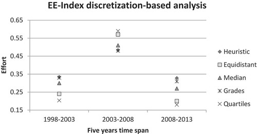
Figure 6 suggests an overall declining trend in the ARE-Index over the period 1998–2013, with a minor upswing in the middle going from 2003 to 2008. What is interesting to note is that in the period between 2003 and 2013, the ARE score displays the “upturn-downturn” behavior similar to the EE-Index, likely for the same reasons. However, it is the reduction in efficiency going from 1998 to 2003 that is reflective of the overall decline in efficiency. Note that the sample variance and the standard deviation for the average relative efficiency scores, a.k.a. ARE-Index for each census period, in Figure 6 are provided in Table 12, and all of them exhibit an almost uniform behavior.

Table 12. ARE-Index and its variance for each census period in Figure 6

Year	E[e’]	Var[e’]
1998	0.66	0.04
2003	0.30	0.04
2008	0.47	0.05
2013	0.29	0.04

Figure 6. ARE-Index for each census period based on the data in Avilés-Sacoto et al.’s (2016) data set for Mexico. Note that the variances for these calculations are not represented in the figure because they all are of the same order of magnitude.

It is important to understand the economic causalities and implications of the results captured in Figures 5 and 6. Intuitively speaking, a steady upward trend could have been expected in both Figures 5 and 6 influenced by the increased trade and production arising from the North American Free Trade Agreement (NAFTA) coming into effect during that period. Reaffirming this intuition is the overall steady growth in Mexican GDP observed in Figure 7. The only year bucking this growth trend is the year 2009, an observation supported by the negative growth/decline in GDP per capita observed for the year in Figure 8. It is important to mention here that Figure 7 represents GDP values computed in international dollars, a type of purchasing power parity (PPP) adjustment; an international dollar “would buy in the cited country a comparable number of goods and services a U.S. dollar would buy in the United States” (World Bank, 2019a).

Figure 7. Mexican GDP per capita adjusted to purchasing power parity (PPP) in current international dollar. Data is taken from the World Bank (World Bank, 2019b). Note that the striped bars represent the corresponding census periods in this study.

Figure 8. Annual change in the GDP per capita of Mexico. Data is taken from the World Bank (World Bank, 2019c). Note that the striped bars represent the corresponding census periods in this study.

Continuing in the same vein of extracting commonalities between the indexes, as can be observed from Figure 5 to 8, the different indexes—EE-Index, ARE-Index, GDP per capita, and annual change in GDP per capita—exhibit unique behaviors that ostensibly are opposing and could have some latent associations. For instance, while the GDP per capita experiences a moderate increase, the ARE-Index exhibits a declining trend. During the same period, the efforts toward improved efficiency increased and then decreased. Several interpretations of these observations are possible. First, it could be that the Mexican economic system was growing based on its natural resources that could have been offsetting the underperformance of human capital and technology-intensive economic activities, and when it did attempt to become more efficient at these latter economic activities, it likely faced a non-favorable economic environment. The second reason could be that Mexico either produced low value-added products or targeted the wrong markets, which limited its capability to improve its overall efficiency of production despite the efforts and expended. In fact, Maloney (2009) believes that Mexico incentivizes the survival of unproductive firms at the expense of the productive ones by penalizing technology adoption to protect jobs; some confirmatory evidence can be found in Cusolito and Maloney’s (2018) work. Third, it could be that several economic activities are downsizing, introducing cost reduction programs, getting rid of assets, or investing in automation in a rush to become more efficient. Fourth, it could be logically argued that labor productivity and efficiency are correlated and that the former could influence the latter. Labor productivity in fact displays trends similar to the EE-Index, increasing in the period 2003–2008 but decreasing in the period 2008–2013 (Financial Times, 2019); the GDP per capita in fact is somewhat plateaued in the period 2008–2013. Finally, it could be that the economic policies are not well aligned with the economic systems and markets, thereby creating balancing causal loops as opposed to growth-reinforcing causal loops. Please note that the above are only conjectures as to what might be causing the GDP per capita on one side and the EE-Index and the ARE-Index on the other side to show potentially opposing behaviors.

Comparing only the ARE-Index and EE-Index, is interesting to note that while the EE-Index exhibits an increase in the efforts to be more efficient for the Mexican Economy over the ten-year period of 1998–2008, the ARE-Index exhibits a declining trend during the same period. What this difference in the behaviors of the EE-Index and the ARE-Index possibly suggests is that even though the economic activities overall are working towards greater efficiency, their collective efforts at the national level seem unsuccessful. This problem may have gone unnoticed had economic growth defined by growth in total output been the primary interest of the observer. The GDP exhibits a growing trend over the period studied as observed in Figure 7; the year-on-year change in GDP in Figure 8 suggests a somewhat constant trajectory. However, GDP growth considered in isolation can be misleading. For instance, in the ten-year period spanning 1998–2008, Mexico (as an oil exporter) enjoyed the benefits of some of the highest oil export prices in its history. Given that oil exports form a big part of Mexico’s GDP matrix, its GDP growth over that period could have been primarily owing to inflated oil prices that may have compensated for the underperformance of other economic activities. This conjecture is supported by the non-increasing and declining trends of the EE-Index and the ARE-Index in Figures 5 and 6, respectively. In fact, since 2008, GDP growth seems to have slowed down, which coincides with the decline in the efforts to be more efficient and average relative efficiency, at least in part because of a significant reduction in oil export prices caused by a supply glut in the oil markets.

To gain more perspective and context that might lay the foundation for a more in-depth analysis in the future, the annual GDP per capita of three countries—Mexico, USA, and China (Figure 8–10, respectively)—are compared. A simple visual inspection reveals how closely the Mexican economy is related to the US economy by way of similar trends, which is not surprising given that the US is Mexico’s biggest trading partner and the GDP reflects explicitly this dependence. Juxtaposed against China’s GDP per capita, more evidence of the dependence of Mexico on the US is evidenced. Considering the period 2003–2007 in fact, while the US GDP per capita monotonically shrunk during this period, that of China grew, probably indicating the increasing share of China’s contribution to trade during the same period. Interestingly, the Mexican economy’s GDP per capita during this period fluctuated. The fluctuation could be likely because of Mexico’s internal production and its own share of global exports compensating for the US shrinkage to a small extent. This finding is actually corroborated by the increase in ARE-Index going from 2003 to 2008 (Figure 6) and the high EE-Index scores (Figure 5). What can also be seen is that over the period 2008–2013, the EE-Index and ARE-Index both decreased, suggesting a reduction in efforts to become more efficient. Coinciding over the same period is a general increase (followed by plateauing) of Mexico’s annual GDP per capita. This observation could be suggestive of the fact that an increase in trade and net exports could have grown at the expense of internal consumption/production and compensated for the same. As also, it possibly suggests internal and external production/consumption not necessarily being collaborative but competing for the same resources for production; this needs to be studied further. Also open to further studies and interpretation could the possible presence of a phase shift dependence between two economies that could be exhibited by any or all of the three indexes studied. For example, the annual GDP per capita of USA and China may have a time-lagged association, in this case, a 3 year one; after all, the 2004 peak of USA coincides with the 2007 peak of China and the 2009 trough of USA coincides with the 2012 trough of China. These are we believe very significant findings that establish the potency of the EE and ARE indexes and their inward-looking focus supplementing, not substituting, the combined internal-external perspective of GDP.

Figure 9. Annual change in the GDP per capita of the USA. Data is taken from the World Bank (World Bank, 2019d). Note that the striped bars represent the corresponding census periods for Mexico.

Figure 10. Annual change in the GDP per capita of China. Data is taken from the World Bank (World Bank, 2019e). Note that the striped bars represent the corresponding census periods for Mexico.

6. Discussion on the choice of the discretization approach

As can be observed in the previous section, the different discretization approaches all led to significantly similar results and thereby established that the EE-Index is insensitive to the choice of discretization approach (see Table 10). Despite this observation, the selection of the discretization method can still cause potential confusion in the minds of the practitioners because its choice can be perceived as arbitrary and lacking any criteria. To address this issue, the authors strongly encourage the use of the 3-state equidistant discretization approach for two reasons. First, the uniformity in its discretization ranges does not favor any one state and thus prevents the introduction of any bias through the act of human choice of range size. Second, given that this approach only considers three states, it minimizes the likelihood of transition matrix infeasibility because the resulting Markov chain is smaller. In addition to these two reasons, we chose the 3-state discretization approach because it is the simplest approach that is also reasonably realistic and serves the purpose of demonstrating the feasibility of these indexes. Further, we did not have any economic logic to choose one of the discretization approaches over the others, which leaves the door open to other scholars to choose the apposite discretization approach that fits best their study requirements and needs.

It must be noted that computational discrepancies are common in the computation of economic indexes worldwide. For instance, central banks and bureaus of statistics often compute GDP and other economic indexes slightly differently manners despite being compliant with the System of National Accounts (SNA). Also known is the fact that the GDP published by the World Bank for a country may differ slightly from the one published by its central bank.

7. Theoretical and practical contributions compared to the standard system of national accounts

The SNA was created to help developed and developing nations to have a common manual on how to compile measures of economic activity. The SNA, for example, encourages the use of the ISIC method to classify industries. Given that the proposed EE-Index and ARE-Index are both based on the NAICS, which in turn is based on the ISIC, it is possible to infer that both indexes are compatible with the general SNA suggestions. The two indexes also further the SNA’s objective to measure all aspects of an economy, including its unobserved components (see Figure 11), and not just a chosen few. Typically, both the observed and unobserved informal aspects of the economic activities in a country are required to gain a holistic understanding of economic development. However, a more in-depth exploration of the EC, IMF, OECD, UN, and WB’s (2009) SNA handbook reveals that the unobserved and formal aspects of an economy are not discussed to the degree they deserve. The EE-Index and the ARE-Index contribute to plugging this gap in the body of knowledge that is the SNA by providing alternative tools to measure the formal and unobserved aspects of an economy like its efforts to be efficient and the effectiveness of these efforts.

Figure 11. The non-observed economy and the informal sector. Adapted from EC, IMF, OECD, UN and WB (2009, p. 471) SNA handbook.

We observed several commonalities and synergies between our work and the SNA handbook. For example, the inputs and outputs in the DMU model (see Figure 3) that form the basis of LDEA computation, and in effect the indexes, are variables such as value-added and labor and capital inputs that have been discussed at length in the handbook. In fact, on account of the inclusion of both labor and capital inputs, both crucial variables for efficiency measurement, the indexes avoid the bias in efficiency measurement that the exclusive inclusion of capital inputs cause per the SNA. Further, these inputs and outputs form a part of the list of variables that the handbook suggests need to be measured regularly and are also in alignment with the SNA’s rules of accounting. In fact, Mexico, the nation that is the chosen subject of this study, has its own system of national accounts that draws upon heavily from the SNA 2008 (Guerrero & Corona, 2018; Van de Ven, 2014). Consequently, the data sourced from Mexican agencies can be expected to be in alignment with the SNA handbook.

8. Conclusions

In this study, an index to ascertain the efforts of industries or economic activities to become more efficient, the EE-Index, was proposed based on an identified need for a metric to complement the GDP in evaluating a national economic system. This composite indicator follows an inside-out approach to measure the aggregate efficiency over a period spanned by two consecutive census periods. Also, this indicator was computed using a combination of multiple inputs/outputs leveled-output-oriented VRS DEA (LDEA) and a stochastic archetype in the form of Markov Chains.

The limited number of assumptions and the nonparametric nature of the combined LDEA-MC methodology makes the proposed dimensionless index easy to compute, accurate given the lack of assumptions of a functional relationship between inputs and outputs, and robust to issues of insufficiency of data. It is believed that the EE-Index captures the behavior of a nation as a complex of several constituent economic activities because while the LDEA captures efficiencies, Markov Chains capture state transition behaviors.

Given that there are several ways to perform the discretization, it was observed, based on the data processed in this work, that going beyond the 4-state discretization resulted in a high probability of transition matrix infeasibility. Conservatively though, the 3-state equidistant discretization is suggested for transition matrix feasibility and because it provides wide ranges and does not require expert judgment thus reducing computational problems and biases. Keeping the focus on the 3-state discretization, of the three methods employing this discretization assessed, the equidistant method was observed to be effective owing to the fact that it reduces the arbitrariness introduced by human intervention in the discretization process.

It is important to note that most cyclical indexes used by Mexico to understand its economic system focus on growth and are of either the coincident or leading type. The EE-Index and the ARE-Index are the first-of-their-kind lagging indicators that are intended to measure not growth or production but efforts and efficiency, respectively. This study, in fact, revealed that growth in Mexican GDP was not always accompanied by a concomitant growth in either efficiencies or efforts of the economic activities, suggesting that the growth could likely be the result of some strong economic activities compensating for the underperformance of several others. This also suggests the existence of grounds for a granular drill-down analysis of underperforming economic activities to tailor policies to enable them to become more efficient and put in more efforts toward that goal. The benefits of more industries or economic activities performing better, thereby boosting Mexico’s growth, based on tailor-made policies cannot be understated.

Overall, the value of this paper is two-fold; (i) it provides two indexes that measure attributes of an economy hitherto unmeasured and provides practitioners with a larger toolbox for diagnosis of the health of an economy and (ii) establishes a novel methodology for the computation of these indexes whilst also providing scope for their further improvement. The authors believe that the EE-Index in combination with the ARE-Index can supplement the GDP and other performance indicators by making visible the hitherto hidden economic dimensions of efforts and efficiency. The authors contend the usefulness of this EE-Index lies in its ability to provide more context to the assessment of national-level economic growth/decline comparison by identifying the synergies and contradictions between the longitudinal values of GDP and itself. It is believed that the EE-Index will enable eventual comparison of and reconciliation between the inside-out and outside-in efficiency scores of an economic system and provide a deeper and richer evaluation of the systemic behavior and interaction of the complex economic activities that compose a national economy. Also, given the relevance of NAFTA to world trade and its value as a template for other free trade agreements around the world, the EE-Index and ARE-Index, in conjunction with GDP per capita, can allow for a more holistic analysis of how the synergies between external and internal economic forces play out by focusing on internal forces as a counterpoint to GDP’s focus on a combination of both.

Cover Image

Source: Author

Acknowledgements

We would like to thank the reviewers and the editorial board for all their invaluable and insightful comments that helped improve our work. We would also like to thank CONACyT, Tecnologico de Monterrey, and Texas Tech University for making this research possible through their support.

Additional information

Funding

The authors received no direct funding for this research.

Notes on contributors

Armando Elizondo-Noriega

Armando Elizondo-Noriega is an active member of the Laboratory of Systems Solutions (LSS) at Texas Tech University (TTU). Founded in 1994, the LSS is a research center designed to provide holistic solutions to the government’s and industry’s systemic problems. The ultimate goal of the LSS is to identify opportunity areas for policy-making at the local, national, and international level factoring in the myriad influences derived from the society, government, industry, and environment. Another goal of the LSS is to develop robust and reliable techniques to address emerging challenges in modern societies, including but not limited to creation of economic indices to understand economic growth and development and assessing economic performance at the industry-level. This paper is the result of collaborative efforts of researchers across several countries and from various universities such as TTU, Tecnologico de Monterrey, Universidad San Francisco de Quito, and Massachussetts Institue of Technology working under the LSS umbrella.

References

- Alqaralleh, H., & Adayleh, R. (2019). The dynamics of the economic cycle with duration dependence: Further evidence from Jordan. Cogent Economics & Finance, 6, 1565609. doi:10.1080/23322039.2019.1565609
- Avilés-Sacoto, S. V., Cook, W. D., Güemes-Castorena, D., & Villareal-González, A. (2016). Setting goals for economic activities in mexico. INFOR: Information Systems and Operational Research, 55, 161–27.
- Bleys, B. (2012). Beyond GDP: Classifying alternatives measures for progress. Social Indicator Research, 109, 355–376. doi:10.1007/s11205-011-9906-6
- Chow, H. K., & Choy, K. M. (1993). A leading economic index for monitoring the Singapore economy. Singapore Economic Review, 38, 81–94.
- Cook, W., & Seiford, L. M. (2009). Data envelopment analysis (DEA) — Thirty years on. European Journal of Operation Research, 192, 1–17. doi:10.1016/j.ejor.2008.01.032
- Cooper, W. W., Seiford, L. M., & Tone, K. (2006). Introduction to data envelopment analysis and its uses: With DEA-solver software and references. United States of America: Springer.
- Cusolito, A. P., & Maloney, W. F. (2018). Productivity revisited: Shifting paradigms in analysis and policy. Washington DC: World Bank.
- Deming, W. E. (2010). Some Theory of Sampling. Dover: United States of America.
- EC, IMF, OECD, UN and WB. (2009). Systems of national accounts (SNA). New York: United Nations.
- Elizondo-Noriega, A., Tiruvengadam, N., Güemes-Castorena, D., Tercero-Gómez, V. G., & Beruvides, M. G. (2019). Identifying the need for an indicator to quantify an economic system’s effort to be efficient: A state-of-the-art analysis. Proceedings of the 2019 IISE Annual Conference, Orlando, FL.
- Emrouznejad, A. (2003). An Alternative DEA measure: A case of OECD countries. Applied Economic Letters, 10, 779–782. doi:10.1080/1350485032000126703
- Financial Times. (2019). Mexico’s economy struggles to reap rewards of good behavior. Retrieved from https://www.ft.com/content/08b6e470-87c0-11e8-bf9e-8771d5404543
- Garcia, A. K. (2018). ¿Qué son los indicadores cíclicos en la economía de México? Retrieved from https://www.eleconomista.com.mx/economia/Que-son-los-indicadores-ciclicos-en-la-economia-de-Mexico-20181105-0063.html?fbclid=IwAR0CuJL_a
- Guerrero, V. M., & Corona, F. (2018). Retropolating some relevant series of Mexico’s System of National Accounts at constant prices: The case of Mexico City’s GDP. Statistica Neerlandica, 72(4), 495–519. doi:10.1111/stan.v72.4
- INEGI (2009). Glosario de Censos Económicos [Data File]. Retrieved from http://www.inegi.org.mx/est/contenidos/espanol/proyectos/censos/ce2009/glosario.asp
- INEGI. (2017). Sistema de Cuentas Nacionales de Mexico: Fuentes y Metodologias. Mexico, DF: Instituto Nacional de Estadistica y Geografia.
- Lequiller, F., & Blades, K. (2004). Comptabilité nationale: Manuel pour étudiants. France: Economica.
- Levy-Algazi, S. (2018). Under-rewarded efforts: The elusive quest for prosperity in Mexico. New York: Inter-American Development Bank.
- Maloney, W. F. (2009). Mexican labor markets: Protection, productivity, and power. In no growth without equity? Inequality, interests, and competition in Mexico. Washington, DC: World Bank and Palgrave Macmillan.
- Mankiw, N. G. (2017). Principles of macroeconomics. United States of America: Cengage Learning.
- Megaravalli, A. V., & Sampagnaro, G.- (2018). Macroeconomic indicators and their impact on stock markets in ASIAN 3: A pooled mean group approach. Cogent Economics & Finance, 6(1), 1432450. doi:10.1080/23322039.2018.1432450
- Michalos, A. C. (2011). Devising an alternative to the GDP: Quality-of-life assessment shouldn't be left to economists. CCPA Monitor (pp. 38–40). Canada: Canadian Center for Policy Alternatives.
- Mollaghasemi, M., & Pet-Edwards, J. (1997). Technical briefing: Making multiple-objective decisions. United States of America: IEEE Computer Society.
- Prieto, A. M., & Zofío, J. L. (2007). Network DEA efficiency in input-output models: With an application to OECD countries. European Journal of Operation Research, 178, 292–304. doi:10.1016/j.ejor.2006.01.015
- Ross, S. M. (2014). Introduction to probability models (11 ed.). San Diego: Elsevier.
- Schunk, D. (2008). Probability predictions of rising real GDP growth and inflation: The usefulness of monetary indicators. Applied Economics, 40, 1139–1149. doi:10.1080/00036840600771247
- Spithoven, A. H. G. M. (2005). Distribution of income and the structure of economy and society. International Journal of Social Economics, 32, 133–154. doi:10.1108/03068290510575685
- Stiglitz, J, Fitoussi, J, & Durand, M. (2018). Beyond gdp : measuring what counts for economic and social performance. Paris: OECD Publishing.
- Stiglitz, J., Sen, A., & Fitoussi, J. P. (2010). Mis-measuring our lives: Why GDP doesn’t add up. United States of America: The New Press.
- The Economist. (2016a). GDP revisions: Rewriting history. Retrieved from https://www.economist. com/briefing/2016/04/30/rewriting-history
- The Economist. (2016b). Measuring economies: The trouble with GDP. Retrieved from https://www .economist.com/briefing/2016/04/30/the-trouble-with-gdp
- Van de Ven, P. (2014). Progress Report on the Implementation of SNA 2008. Basel: Organization of Economic Cooperation and Develoment.
- Van den Bergh, J. C. J. M. (2009). The GDP Paradox. Journal of Economic Psychology, 30, 117–135. doi:10.1016/j.joep.2008.12.001
- World Bank (2019a). What is an “international dollar”? [Data file]. Retrieved from https://datahelpdesk.worldbank.org/knowledgebase/articles/114944-what-is-an-international-dollar
- World Bank (2019b). Mexico’s GDP per capita PPP (current international $)[Data file]. Retrieved from https://data.worldbank.org/indicator/NY.GDP.PCAP.PP.CD?locations= MX
- World Bank (2019c). Mexico’s GDP per capita growth (annual %)[Data file]. Retrieved from: https://data.worldbank.org/indicator/NY.GDP.PCAP.KD.ZG?locations=MX
- World Bank (2019d). United States’s GDP per capita growth (annual %)[Data file]. Retrieved from https://data.worldworldbank.org/indicator/NY.GDP.PCAP.KD.ZG?locations=US
- World Bank (2019e). China’s GDP per capita growth (annual %)[Data file]. Retrieved from https://data.worldbank.org/indicator/NY.GDP.PCAP.KD.ZG?locations=CN