Financial contracting and misreporting with limited enforcement, firm financing and growth

Abstract

This article employs a dynamic stochastic general equilibrium framework to examine asymmetric information and limited contract enforcement in financial markets, where firms have access to both internal and external sources of finance. It considers limited enforcement of financial contract in the form of firm’s ability to misreport and default on output when it is still solvent, that is, a form of institutional weaknesses in holding defaulters to account. The model shows how institutional weakness in the form of limited enforceability of financial contracts affects fluctuations in key macroeconomic variables such as output, employment and investment via its impact on interest rates, risk premium, default risk and leverage. The findings show that limited contract enforcement amplifies the effects of shocks and lower small firm funding. The sensitivity analysis shows that weak contract enforcement affects firm growth and also leads to welfare losses to the society. This study is relevant for developing countries, where there is often poor quality of institutions and the paper suggests that improving such quality has the potential to improve the prospects of such countries.

Keywords:

• Contracting
• institutional weakness
• limited enforcement
• misreporting
• financing

JEL:

• B26
• D86
• E32
• K12
• K42
• O43

PUBLIC INTEREST STATEMENT

In this paper, we examine the relationship between firm investment and poor-quality institutions. We consider limited enforcement of financial contract as a form of institutional weakness in holding defaulters to account if firms default and misreport on output when it is still solvent. Such poor institutions have the tendency to affect lenders and also firms’ access to funds and also affect fluctuations in key macroeconomic variables such as output, employment and investment via its negative impact on interest rates, risk premium, analysis shows default risk and leverage. Our analysis shows that when this phenomenon is allowed to persist, firm growth and welfare gains to the society are hampered. This study is particularly relevant for developing countries, where there is often poor quality of institutions, and the paper suggests that improving such quality has the potential to improve the prospects of such countries.

1. Introduction

The role that financial factors and financial development play in economic activity has long been documented in the business-cycle literature (Carlstrom & Fuerst, 1997, 1998; Gertler, 1988). Some of these roles are smoothing fluctuations and enhancing productive efficiency. However, these roles hinge crucially on the existence of good institutions to ensure that financial contracts are well enforced. Hence, when the market for loans has an imperfection such that agents can choose to default on their debt at an exogenous cost governed by the quality of institutions, economic development becomes undermined. Levine, Loayza, and Beck (2000) find that contract enforcement promotes financial development, while the latter is conducive to economic growth. However, developing economies do not only have weak legal institutions to enforce contracts but are also characterised by high lending rates, unavailability of capital and a generally risky investment environment.

The growth of firms depends on the level of access to external financing which in turn depends on informational asymmetries and contractual arrangements between investors and entrepreneurs. The average scale of production increases with the quality of enforcement and the importance of limited enforcement rises with the importance of capital in production¹ (Amaral & Quintin, 2010). Costly contract enforcement means that lenders receive less compensation when firms default which then impacts on default risk. In turn, this will alter contract arrangements and vice versa. The consequences of limited enforcement of contracts for borrowing and lending are much severe when coupled with asymmetries of information.

Limited enforceability of contracts is especially important for new and smaller firms constrained by working capital and collateral problems and have to rely mostly on external funding. This has implications for both firm level and aggregate growth and welfare. It is argued that the enforceability of financial contracts can help explain the growth of firms (Albuquerque & Hopenhayn, 2000). Weakness in contract enforcement hampers small firms access to finance, and such firms are forced to rely mainly on self-funding and to operate on a small scale due to credit constraints which deny them of external funding (Amaral & Quintin, 2010). In particular, productive firms are mostly financially constrained in countries with imperfect financial markets. Such firms are impaired from borrowing enough to reach their optimal sizes (Steinberg, 2013).

In spite of the above, little research has been conducted on exploring the interlinkages between limited contract enforcement, asymmetric information, financial intermediation and firm funding. The present paper seeks to do so within the context of a Dynamic Stochastic General Equilibrium (DSGE) model. Specifically, it studies the implications of limited enforcement for financial intermediation, small firm funding, economic growth and welfare. This objective is achieved by modifying the models of Carlstrom and Fuerst (1997) to allow for the imperfect enforcement on loan contracts. In doing so, the study draws upon the works of Khan and Ravikumar (2001), Marcet and Marimon (1992), Castro, Clementi, and MacDonald (2004), Quintin (2000), Cooley, Marimon, and Quadrini (2003), Boedo, Senkal, and D’Erasmo (2011), Bernanke, Gertler, and Gilchrist (1999), De Fiore, Teles, and Tristani (2011), and Amaral and Quintin (2010). This study is similar to Cooley et al. (2003) on the basis of the assumption that firms which default in one period are not excluded from the financial market in subsequent periods. Additionally, the assumption that firms can use funds from defaulting in next period production given that they are not excluded from the financial market is upheld. The study, therefore, argues that better contract enforcement helps in the growth and the transfer of resources to lenders which is accessed via banks by small firms to finance investment projects, contrary to the view of Marcet and Marimon (1992) that better contract enforcement leads to less growth.

As advanced earlier, the study follows Bernanke et al. (1999), De Fiore et al. (2011), Carlstrom and Fuerst (1998, 2001), and Carlstrom, Fuerst, and Paustian (2010) on asymmetric information in financial markets. According to these authors to engage in investment opportunities, risk-neutral entrepreneurs have the potential to access funds from lenders. However, this funding is constrained because of agency costs involved. Lenders are risk-averse households who offer loans to entrepreneurs through the Capital Market Fund (CMF)/Bank. A key feature of the model used in this study is the distinction between the monitoring cost and enforcement cost, in the event that an entrepreneur defaults on its loan. We do so by allowing for the possibility of the firm to default on borrowed funds when it is still solvent. At the same time, a defaulting firm faces the prospect of being punished when caught. This punishment involves the confiscation of some fraction of a firm’s capital output, dependent on the quality of legal institutions. The results of the paper emphasise the role that limited enforcement plays in determining the default risk and access to funding by small firms. One key finding of this paper is that the probability of default, risk premium and the resulting cost of borrowing all increase monotonically with the degree of limited contract enforcement. We show how the degree of limited contract enforcement affects business-cycle fluctuations and specifically amplifies the effects of shocks on the economy. We also find that limited enforcement coupled with the ability of firms to default when solvent creates a problem for the establishment and growth of smaller firms as a result of over-accumulation of internal funds by larger firms. Given that firms are able to default when solvent, and that households provide loanable funds, we also demonstrate that limited enforcement is associated with welfare loss to households and the economy in general.

The rest of the paper is organised as follows. In Section 2, we set out the theoretical model used to study the relationship between firm funding and limited enforcement of contracts and provide the solution. We then calibrate the model and present the findings. In Section 3, we make some concluding remarks.

2. The investment model

The model based on Carlstrom and Fuerst (1997) is extended to allow for imperfect contract enforcement. The model economy consists of a continuum of agents of unit mass, a fraction $(1-\eta )$ of which are risk-averse households and a fraction $\eta$ are risk-neutral entrepreneurs (or capital-producing firms). Households who own (shares in) the consumption-good producing firms also supply labour and rent capital to these firms, invest in capital and advance intra-period loans via Capital Market Fund (CMF)/Bank to entrepreneurs. Entrepreneurs invest in (produce) capital goods using net worth and external funds in the form of loans from the CMF/Bank. Following Gertler and Bernanke (1989), this paper assumes informational asymmetries in creating capital goods (investment) by the entrepreneurs. In what follows, the financial contracting problem in a partial equilibrium setting is developed section 2.1. This sets out the decision to invest and the decision to default and misreport by the entrepreneur. The next section, 2.2, sets out the general equilibrium environment (comprising households, entrepreneurs, firms and the CMF/Bank) using the optimal results from the financial contracting problem.

2.1. The financial contract

This section discusses the financial contract in a partial equilibrium setting. It is one period in length, negotiated at the beginning of the period and resolved by the end of the same period. The contract involves the entrepreneur and the lender both of which are risk neutral.² The lender has resources that he can lend to an entrepreneur with some positive net worth. Each entrepreneur is endowed with a stochastic technology that transforms $i$ consumption goods into $\omega i$ units of capital, where $\omega$ is idiosyncratic technology shock. The shock $\omega$, is $i.i.d.$ across time and across entrepreneurs, with cumulative distribution function $\mathrm{\Phi }$ and probability density function $\varphi$. We assume $\omega$ has mean $\mathbb{E}[\omega ]=1$, standard deviation ${\sigma }_{\omega }$, and is privately observed by the entrepreneur, but others can privately observe $\omega$ only after paying the monitoring cost of $\mu i$ capital units. The monitoring cost denominated in terms of capital is proportional to $i$ and independent of the realisation of $\omega$. To ensure that the asymmetric information in the model is important, we assume that net worth is sufficiently small so that entrepreneurs would like to receive some external financing to finance investment. Otherwise, entrepreneurs would not need to borrow to finance investment. To finance the investment $i$, the entrepreneur uses its net worth n and borrows $(i-n)$ consumption goods and agrees to repay $(1+r^k)(i-n)$ capital goods to the lender, where $r^k$ is the lending rate. The entrepreneur defaults at the end of the period if the realisation of $\omega$ is low. However, if the entrepreneur defaults, it can “hide” a fraction $\zeta$ of the capital. The inability of lenders to recover this “hidden” capital due to weakness in legal institutions is termed limited contract enforcement. While monitoring cost ($\mu i$ capital units) pertains to the cost of monitoring borrowers, limited enforcement involves the “cost” that lenders have to incur (which is equivalent to the volume of this “hidden” capital) in order to recover the “hidden” capital. Therefore, if the entrepreneur does not default, it receives:

(1) $\omega i-(1+r^k)(i-n)$(1)

capital goods, which it can then sell at the price q (the price of aggregate capital). If the entrepreneur defaults, however, it receives:

(2) $\zeta \omega i$(2)

Comparing Equations (1)(1) $\omega i-(1+r^k)(i-n)$(1) and (2(2) $\zeta \omega i$(2) ), the entrepreneur will default if and only if

$(1-\zeta )\omega i<(1+r^k)(i-n)$

This is equivalent to Carlstrom and Fuerst (1997) when $\zeta =0$.

It is then possible to define a default threshold $\bar{\omega }$ such that the entrepreneur will default for $\omega <\bar{\omega }$ and not default for $\omega \ge \bar{\omega }$. This threshold is determined by:

(3) $(1-\zeta )\bar{\omega }i=(1+r^k)(i-n)$(3)

If $\omega \ge \bar{\omega }$, the entrepreneur does not default and receives $\omega i-(1+r^k)(i-n)$. If $\omega <\bar{\omega }$, the entrepreneur defaults and he receives $\zeta \omega i$. In both cases, the entrepreneur can then sell the capital it has at the price $q$. Therefore, expected entrepreneurial income is given by

$q\left[{\int }_0^{\bar{\omega }}\zeta \omega id\mathrm{\Phi }(\omega )+{\int }_{\bar{\omega }}^{\mathrm{\infty }}\left[\omega i-(1+r^k)(i-n)\right]d\mathrm{\Phi }(\omega )\right]$

Using Equation (3)(3) $(1-\zeta )\bar{\omega }i=(1+r^k)(i-n)$(3) to substitute for $(1+r^k)(i-n)$, this becomes:

$qi\left[\zeta {\int }_0^{\bar{\omega }}\omega d\mathrm{\Phi }(\omega )+{\int }_{\bar{\omega }}^{\mathrm{\infty }}\omega d\mathrm{\Phi }(\omega )-(1-\zeta )\bar{\omega }(1-\mathrm{\Phi }(\bar{\omega }))\right]$

Therefore, as a result of this contract, the entrepreneur expects to receive $qif(\bar{\omega })$, where $f(\bar{\omega })$ is the fraction of the expected capital output received by the entrepreneur. This is defined to be:

(4) $f(\bar{\omega })=1-(1-\zeta )\left[{\int }_0^{\bar{\omega }}\omega d\mathrm{\Phi }(\omega )+\bar{\omega }(1-\mathrm{\Phi }(\bar{\omega }))\right]$(4)

Similarly, for the lender, if $\omega \ge \bar{\omega }$, the entrepreneur does not default and the lender receives $(1+r^k)(i-n)$ in capital units. If $\omega <\bar{\omega }$, the entrepreneur defaults and the lender receives $((1-\zeta )\omega -\mu )i$ capital units. Then, expected lender’s income is given by

$q\left[{\int }_0^{\bar{\omega }}((1-\zeta )\omega -\mu )id\mathrm{\Phi }(\omega )+{\int }_{\bar{\omega }}^{\mathrm{\infty }}(1+r^k)(i-n)d\mathrm{\Phi }(\omega )\right]$

Again, using Equation (3)(3) $(1-\zeta )\bar{\omega }i=(1+r^k)(i-n)$(3) , the expected lender’s income simplifies to

$qi\left[(1-\zeta )\left\{{\int }_0^{\bar{\omega }}\omega d\mathrm{\Phi }(\omega )+\bar{\omega }(1-\mathrm{\Phi }(\bar{\omega }))\right\}-\mu \mathrm{\Phi }(\bar{\omega })\right]$

As a result of this contract, the lender expects to receive $qig(\bar{\omega })$, where $g(\bar{\omega })$ is the fraction of the expected capital output received by the lender. This is defined to be:

(5) $g(\bar{\omega })=(1-\zeta )\left[{\int }_0^{\bar{\omega }}\omega d\mathrm{\Phi }(\bar{\omega })+\bar{\omega }(1-\mathrm{\Phi }(\bar{\omega }))\right]-\mu \mathrm{\Phi }(\bar{\omega })$(5)

Moreover, using Equations (4)(4) $f(\bar{\omega })=1-(1-\zeta )\left[{\int }_0^{\bar{\omega }}\omega d\mathrm{\Phi }(\omega )+\bar{\omega }(1-\mathrm{\Phi }(\bar{\omega }))\right]$(4) and (5(5) $g(\bar{\omega })=(1-\zeta )\left[{\int }_0^{\bar{\omega }}\omega d\mathrm{\Phi }(\bar{\omega })+\bar{\omega }(1-\mathrm{\Phi }(\bar{\omega }))\right]-\mu \mathrm{\Phi }(\bar{\omega })$(5) ) we arrive at

(6) $f(\bar{\omega })+g(\bar{\omega })=1-\mu \mathrm{\Phi }(\bar{\omega })$(6)

This implies that, on average, monitoring results in the destruction of some of the produced capital, and the remainder of this capital is split between the entrepreneur and the lender.

The optimal contract is given by the pair $(i,\bar{\omega })$ (taking as given net worth $n$ and capital price $q)$ which solves:

$\underset{i,\bar{\omega }}{max}qif(\bar{\omega })$

subject to

$qig(\bar{\omega })\ge i-n{\mathrm{L}\mathrm{e}\mathrm{n}\mathrm{d}\mathrm{e}\mathrm{r}}^{\prime }\mathrm{s}\mathrm{P}\mathrm{a}\mathrm{r}\mathrm{t}\mathrm{i}\mathrm{c}\mathrm{i}\mathrm{p}\mathrm{a}\mathrm{t}\mathrm{i}\mathrm{o}\mathrm{n}\mathrm{c}\mathrm{o}\mathrm{n}\mathrm{s}\mathrm{t}\mathrm{r}\mathrm{a}\mathrm{i}\mathrm{n}\mathrm{t}$

$qif(\bar{\omega })\ge n{\mathrm{E}\mathrm{n}\mathrm{t}\mathrm{r}\mathrm{e}\mathrm{p}\mathrm{r}\mathrm{e}\mathrm{n}\mathrm{e}\mathrm{u}\mathrm{r}}^{\prime }\mathrm{s}\mathrm{P}\mathrm{a}\mathrm{r}\mathrm{t}\mathrm{i}\mathrm{c}\mathrm{i}\mathrm{p}\mathrm{a}\mathrm{t}\mathrm{i}\mathrm{o}\mathrm{n}\mathrm{c}\mathrm{o}\mathrm{n}\mathrm{s}\mathrm{t}\mathrm{r}\mathrm{a}\mathrm{i}\mathrm{n}\mathrm{t},\mathrm{w}\mathrm{h}\mathrm{i}\mathrm{c}\mathrm{h}\mathrm{i}\mathrm{s}\mathrm{a}\mathrm{l}\mathrm{w}\mathrm{a}\mathrm{y}\mathrm{s}\mathrm{s}\mathrm{a}\mathrm{t}\mathrm{i}\mathrm{s}\mathrm{f}\mathrm{i}\mathrm{e}\mathrm{d}$

The solution³ to the optimal contract is the following:

(7) $q\left[1-\mu \mathrm{\Phi }(\bar{\omega })-\frac{\mu \varphi (\bar{\omega })f(\bar{\omega })}{(1-\zeta )(1-\mathrm{\Phi }(\bar{\omega }))}\right]=1$(7)

This can also be written as:

$q\left[1-\mu \mathrm{\Phi }(\bar{\omega })+\mu \varphi (\bar{\omega })\frac{f(\bar{\omega })}{f^{\prime }(\bar{\omega })}\right]=1$

This implicitly defines a function $\bar{\omega }(q)$. Then, given $\bar{\omega }(q)$, we can solve for optimal investment using the participation constraint of the lender:

(8) $i(q,n)=\frac{n}{1-qg(\bar{\omega }(q))}$(8)

Substituting in $\bar{\omega }(q)$, this gives us the function $i(q,n)$, which represents the optimal amount of consumption goods placed into the capital-producing technology (given $q$ and net worth $n$). The expected capital output is then given by:

$I^s(q,n)\equiv i(q,n)\left[1-\mu \mathrm{\Phi }(\bar{\omega }(q))\right]$

This can be interpreted as the investment supply function. This implies that the supply function of entrepreneurs aggregates. Aggregate investment depends only on the economy-wide price of capital $q$ and aggregate net worth. It can then be shown that $\mathrm{\partial }{I}^s/\mathrm{\partial }q>0$ and $\mathrm{\partial }{I}^s/\mathrm{\partial }n>0$.

An entrepreneur who receives a loan of one unit of consumption good from the household (via CMF/bank) expects to make a risky return of $q(1+r^k)$ consumption good at the end of the investment period. Therefore, the risk premium of the model is $q(1+r^k)-1$. Substituting for $(1+r^k)$ using Equation (3)(3) $(1-\zeta )\bar{\omega }i=(1+r^k)(i-n)$(3) , the risk premium can also be written as:

$q(1+r^k)-1=q(1-\zeta )\bar{\omega }\frac{i}{i-n}-1$

Finally, we may define leverage $z$, of the entrepreneur as the ratio of external funding $(i-n)$ to the net worth $n$ of the entrepreneur. This is given by

$z=\frac{i-n}{n}$

Then, using Equation (8)(8) $i(q,n)=\frac{n}{1-qg(\bar{\omega }(q))}$(8) this can be re-written as:

$z=\frac{qg(\bar{\omega }(q))}{1-qg(\bar{\omega }(q))}$

2.2. The general equilibrium model

We now embed the contracting problem into a standard real business-cycle (RBC) model. We further assume that, using consumption goods, new capital is created at the end of the period with a non-stochastic one-to-one transformation rate. The newly produced capital is then utilised in the next period. We use the same timing in this model. The one-to-one transformation assumption is replaced with the contracting problem so that a household who wants to purchase capital must first fund the production of capital (an entrepreneurial project), which is subject to agency problems.

The economy consists of a continuum of agents of unit mass, a fraction $(1-\eta )$ of which are households and a fraction $\eta$ are entrepreneurs. Firms produce the single consumption good, but it is assumed that these consumption-producing firms are not subject to any agency problems.

2.2.1. Households

Households are infinitely lived, with preferences:

${\mathbb{E}}_0\left[\sum _{t=0}^{\mathrm{\infty }}{\beta }^{t}U(c_t,1-L_t)\right]$

where $U(c_t,1-L_t)=ln(c_t)+\nu (1-L_t)$ is the instantaneous utility function, $\mathbb{E}$ is the expectation operator conditional on period 0 information, $\beta \in (0,1)$ is the discount factor, $c_t$ is household consumption, $L_t$ is labour. Households supply labour to consumption-producing firms at wage rate $w_t$, rent their accumulated capital holdings to consumption-producing firms at rental rate $r_t$, purchase consumption from these firms at the price 1 (note that consumption is the numeraire) and purchase new capital goods at a price of $q_t$. Within the period, households also lend to entrepreneurs (through the CMF/Bank) to help finance the production of capital. Households who own (shares in) the consumption-good producing firms then purchase capital goods at the end of the period with the assistance of CMF/Bank.

The budget constraint faced by the household is then:

$c_t+q_t\left[k_{t+1}^h-(1-\delta )k_t^h\right]=w_t{L}_t+r_t{k}_t^h$

where $k_t^h$ is the stock of capital owned by the representative household. The profits of the CMF/bank are not included here, because they will be zero.

Optimal consumption-labour decision is determined by the following:

$w_t=\frac{U_L(c_t,1-L_t)}{U_c(c_t,1-L_t)}$

Also, optimal⁴ household consumption-investment decision is determined by the following:

$q_t{U}_c(c_t,1-L_t)=\beta {\mathbb{E}}_t\left\{U_c(c_{t+1},1-L_{t+1})\left[q_{t+1}(1-\delta )+r_{t+1}\right]\right\}$

2.2.2. Consumption-good producing firms

There are a continuum of consumption-producing firms in the economy who utilise a standard production function with constant returns to scale (CRS) specified as:

$Y_t=A_t{K}_t^{{\alpha }_K}{H}_t^{{\alpha }_H}{H}_t^{e{\alpha }_e}$

where $Y_t$ is aggregate output of the consumption good. ${\alpha }_K,{\alpha }_H$ and ${\alpha }_e$ are the shares of $K_t$ (the aggregate capital stock, including entrepreneurial capital), $H_t$ (the aggregate supply of household labour) and $H_t^e$ (the aggregate supply of entrepreneurial labour), respectively. $A_t$ is stochastic aggregate productivity and evolves according to $log(A_t)=(1-{\rho }_A)A+{\rho }_{A}log(A_{t-1})+{\epsilon }_t$, where ${\epsilon }_t$ is a serially uncorrelated, $i.i.d.$ and normally distributed shock; and ${\rho }_A$ is the autocorrelation coefficient. This consumption-good producing technology is assumed to be Cobb–Douglas (details are discussed in section 2.3). Perfect competition in factor markets ensures that factor prices are equal to their respective marginal products: $r_t=A_t{F}_1(K_t,H_t,H_t^e)$, $w_t=A_t{F}_2(K_t,H_t,H_t^e)$, and $w_t^e=A_t{F}_3(K_t,H_t,H_t^e)$, where $w_t^e$ is the wage rate for entrepreneurial labour. As explained in Carlstrom and Fuerst (1997), the assumption of entrepreneurial labour income is to ensure that each entrepreneur has a non-zero level of net worth. This is because the financial contracting problem will not be well defined for any zero levels of net worth.

2.2.3. Entrepreneurs

Entrepreneurs are long-lived and risk-neutral. Without any restrictions, entrepreneurs will want to accumulate enough capital so that they are completely self-financed and avoid agency costs by postponing consumption. To prevent this, we follow on Carlstrom and Fuerst (1997) and assume that entrepreneurs discount the future more heavily than households.⁵ Following the risk neutrality assumption, entrepreneurs maximise the following objective function:

(9) ${\mathbb{E}}_0\left[\sum _{t=0}^{\mathrm{\infty }}{(\beta \gamma )}^t{c}_t^e\right]$(9)

where $c_t^e$ is entrepreneurial consumption, and $\gamma \in (0,1)$ denotes the additional rate of discounting for entrepreneurs to ensure that $\beta \gamma <\beta$. At the beginning of the period the entrepreneur rents his previously accumulated capital and also inelastically supplies labour, which we assume to be unity, to consumption-good producing firms. The entrepreneur then sells his remaining undepreciated capital to households for consumption goods. The net worth of the entrepreneur at the end of the transaction period is given by:

$n_t=w_t^e+k_t^e\left[q_t(1-\delta )+r_t\right]$

where $k_t^e$ refers to the capital holdings of the individual entrepreneur at the beginning of the period. To undertake investment, the entrepreneur uses this net worth to form the basis for any loan agreement that he will enter into with the lender. Risk neutrality and the high internal return ensure the entrepreneur pours his entire net worth into the capital-producing technology and borrows from the household (via the CMF/Bank). Given the financial contract from Section 2.1, the entrepreneur chooses $i_t=i(q_t,n_t)$, where $i(q,n)$ is defined in Equation (8)(8) $i(q,n)=\frac{n}{1-qg(\bar{\omega }(q))}$(8) . There is also an associated cutoff ${\bar{\omega }}_t=\bar{\omega }(q_t)$, where $\bar{\omega }(q)$ is implicitly defined by Equation (7)(7) $q\left[1-\mu \mathrm{\Phi }(\bar{\omega })-\frac{\mu \varphi (\bar{\omega })f(\bar{\omega })}{(1-\zeta )(1-\mathrm{\Phi }(\bar{\omega }))}\right]=1$(7) , given this investment. Let $x_t$ denote the realised payoff to the entrepreneur given by:

$x=\left\{\begin{array}{cc}\omega i-(1+r^k)(i-n)=\omega i-(1-\zeta )\bar{\omega }i=(\omega -(1-\zeta )\bar{\omega })i& \mathrm{i}\mathrm{f}\omega \ge \bar{\omega }\\ \zeta \omega i& \mathrm{i}\mathrm{f}\omega <\bar{\omega }\end{array}\right.$

Then, given $x$, the entrepreneur makes the consumption decision:

$c_t^e+q_t{k}_{t+1}^e=q_t{x}_t$

Let ${\bar{c}}_t^e$ denote average entrepreneurial consumption. Then, $\eta {\bar{c}}_t^e$ is aggregate entrepreneurial consumption. Aggregating across the budget constraints of all entrepreneurs, we get:

$\eta {\bar{c}}_t^e+q_t{K}_{t+1}^e=q_t\frac{N_t}{1-q_{t}g(\bar{\omega }(q_t))}f(\bar{\omega }(q_t))$

where $K_{t+1}^e$ is aggregate entrepreneurial capital stock and $N_t$ is aggregate entrepreneurial net worth. Aggregate net worth is $N_t=\eta w_t^e+K_t^e(q_t(1-\delta )+r_t)$. Re-arranging, tomorrow’s aggregate entrepreneurial capital stock $(K_{t+1}^e)$ is given by:

(10) $K_{t+1}^e=\left[\eta w_t^e+K_t^e(q_t(1-\delta )+r_t)\right]\frac{f(\bar{\omega }(q_t))}{1-q_{t}g(\bar{\omega }(q_t))}-\frac{\eta {\bar{c}}_t^e}{q_t}$(10)

Dividing through by $\eta$ (the mass of entrepreneurs), we get:

${\bar{k}}_{t+1}^e={\bar{n}}_t\frac{f(\bar{\omega }(q_t))}{1-q_{t}g(\bar{\omega }(q_t))}-\frac{{\bar{c}}_t^e}{q_t}$

where ${\bar{n}}_t=w_t^e+{\bar{k}}_t^e\left[q_t(1-\delta )+r_t\right]$ is average entrepreneurial net worth and ${\bar{k}}_t^e=K_t^e/\eta$ is the average stock of capital owned by entrepreneurs.

Maximising the entrepreneur’s utility in Equation (9)(9) ${\mathbb{E}}_0\left[\sum _{t=0}^{\mathrm{\infty }}{(\beta \gamma )}^t{c}_t^e\right]$(9) subject to the aggregate entrepreneurial capital stock in Equation (10)(10) $K_{t+1}^e=\left[\eta w_t^e+K_t^e(q_t(1-\delta )+r_t)\right]\frac{f(\bar{\omega }(q_t))}{1-q_{t}g(\bar{\omega }(q_t))}-\frac{\eta {\bar{c}}_t^e}{q_t}$(10) (indicated in Appendix 4.3) gives the entrepreneur’s Euler equation:

$q_t=\beta \gamma {\mathbb{E}}_t\left\{\left[q_{t+1}(1-\delta )+r_{t+1}\right]\frac{q_{t+1}f({\bar{\omega }}_{t+1})}{1-q_{t+1}g({\bar{\omega }}_{t+1})}\right\}$

The first term (in brackets) represents the market return on capital whilst the second term denotes the additional return on internal funds.

2.2.4. Capital market fund (CMF)/bank

The CMF/Bank lends $(i_t(q_t,n_t)-n_t)$ consumption goods to each entrepreneur with a net worth $n_t$ (measured in consumption units). Let $N_t$ denote aggregate entrepreneurial net worth. Since the investment function in Equation (8)(8) $i(q,n)=\frac{n}{1-qg(\bar{\omega }(q))}$(8) is linear in net worth, aggregate lending is $\left(\frac{q_{t}g(\bar{\omega }(q_t))}{1-q_{t}g(\bar{\omega }(q_t))}\right)N_t$, denominated in terms of consumption units.

At the end of the period, $\omega$ is realised for all firms and the expected proceeds from each individual entrepreneur is $q_{t}i(q_t,n_t)g(\bar{\omega }(q_t))$. Given that $i(q_t,n_t)$ is linear in $n_t$, this aggregates. Therefore, the total proceeds to the CMF/Bank are $\frac{N_t}{1-q_{t}g(\bar{\omega }(q_t))}{q}_{t}g(\bar{\omega }(q_t))$. Comparing aggregate lending to total proceeds of the CMF/Bank, its profits are zero. This is because, in the optimal contracting problem, the lender’s participation constraint holds with equality.

2.2.5. Market-clearing conditions

We close the model with the market-clearing conditions. The economy is characterised by four markets: two labour markets, a consumption-goods market, and a capital-goods market. Labour market clearing for the consumption-goods sector ensures:

$H_t=(1-\eta )L_t$

$H_t^e=\eta$

Consumption-good market clearing implies:

$(1-\eta )c_t+\eta {\bar{c}}_t^e+\eta {\bar{i}}_t=Y_t$

where $c_t$ is the representative household’s consumption, ${\bar{c}}_t^e$ is average entrepreneurial consumption, and ${\bar{i}}_t$ is average entrepreneurial investment. Finally, the capital-goods market clearing implies:

$K_{t+1}=(1-\delta )K_t+\eta {\bar{i}}_t\left[1-\mu \mathrm{\Phi }({\bar{\omega }}_t)\right]$

where aggregate capital $K_t=(1-\eta )k_t^h+\eta {\bar{k}}_t^e$ includes both household and entrepreneurial capital.

2.2.6. Recursive competitive equilibrium

A recursive competitive equilibrium consists of the following decision rules: $k_{t+1}^h,{\bar{k}}_{t+1}^e,$ $K_{t+1},K_{t+1}^e,q_t,{\bar{n}}_t,{\bar{i}}_t,{\bar{\omega }}_t,{\bar{c}}_t^e,c_t,r_t,w_t,w_t^e,H_t,H_t^e,L_t,\mathrm{a}\mathrm{n}\mathrm{d}{Y}_t$, such that these decision rules are stationary functions of $(K_t,K_t^e,A_t)$ and the following conditions are satisfied:

(1) Optimality conditions for household labour supply:

$\frac{U_L(c_t,1-L_t)}{U_c(c_t,1-L_t)}=w_t$

(2) Optimality conditions for household investment:

$q_t{U}_c(c_t,1-L_t)=\beta {\mathbb{E}}_t{U}_c(c_{t+1},1-L_{t+1})\left[q_{t+1}(1-\delta )+r_{t+1}\right]$

(3) Market clearing for capital good market:

$K_{t+1}=(1-\delta )K_t+\eta {\bar{i}}_t\left[1-\mu \mathrm{\Phi }({\bar{\omega }}_t)\right]$

(4) Market clearing for consumption:

$(1-\eta )c_t+\eta {\bar{c}}_t^e+\eta {\bar{i}}_t=Y_t$

(5) First-order conditions defining ${\bar{\omega }}_t=\bar{\omega }(q_t)$:

$q_t\left[1-\mu \mathrm{\Phi }({\bar{\omega }}_t)+\mu \varphi ({\bar{\omega }}_t)\frac{f({\bar{\omega }}_t)}{f^{\prime }({\bar{\omega }}_t)}\right]=1$

(6) Average investment ${\bar{i}}_t$ set optimally (given average net worth $n_t$):

${\bar{i}}_t=i(q_t,{\bar{n}}_t)=\frac{{\bar{n}}_t}{1-q_{t}g({\bar{\omega }}_t)}$

(7) Average entrepreneurial net worth ${\bar{n}}_t$:

${\bar{n}}_t=w_t^e+{\bar{k}}_t^e\left[q_t(1-\delta )+r_t\right]$

(8) Next period’s average entrepreneurial capital ${\bar{k}}_{t+1}^e$:

${\bar{k}}_{t+1}^e={\bar{n}}_t\frac{f({\bar{\omega }}_t)}{1-q_{t}g({\bar{\omega }}_t)}-\frac{{\bar{c}}_t^e}{q_t}$

(9) Next period’s aggregate entrepreneurial capital $K_{t+1}^e$:

$K_{t+1}^e=\left[\eta w_t^e+K_t^e(q_t(1-\delta )+r_t)\right]\frac{f(\bar{\omega }(q_t))}{1-q_{t}g(\bar{\omega }(q_t))}-\frac{\eta {\bar{c}}_t^e}{q_t}$

(10) First order conditions for entrepreneurial consumption:

$q_t=\beta \gamma {\mathbb{E}}_t\left\{\left[q_{t+1}(1-\delta )+r_{t+1}\right]\frac{q_{t+1}f({\bar{\omega }}_{t+1})}{1-q_{t+1}g({\bar{\omega }}_{t+1})}\right\}$

(11) Aggregate capital:

$K_{t+1}=(1-\eta )k_{t+1}^h+\eta {\bar{k}}_{t+1}^e$

(12) Labour market clearing for the consumption-goods sector:

$H_t=(1-\eta )L_t$

$H_t^e=\eta$

(13) Factor markets:

$r_t=A_t{F}_1(K_t,H_t,H_t^e)$

$w_t=A_t{F}_2(K_t,H_t,H_t^e)$

$w_t^e=A_t{F}_3(K_t,H_t,H_t^e)$

2.3. Calibration and results

We simulate and solve the model in Dynare. To simulate the model, we first need to calibrate it. The calibration (Table 1) is at the non-stochastic steady state. As noted earlier, we assume that utility is logarithmic in consumption and linear in leisure. Following Carlstrom and Fuerst (1997), we choose $\nu$, disutility of labour supply parameter, to be $2.52$ so that $L=0.3$. We normalise $\eta$, fraction of entrepreneurs, to be $10\mathrm{\%}$.

The Cobb–Douglas consumption-good producing technology has $36\mathrm{\%}$ as share of capital and $63.99\mathrm{\%}$ as share of household labour. Drawing on Carlstrom and Fuerst (1997) and Carlstrom and Fuerst (1998), we set $0.01\mathrm{\%}$ as the share of entrepreneurial labour. As stated earlier, this is also to, purposely, ensure that each entrepreneur always has a positive level of net worth. The autocorrelation coefficient ${\rho }_A$ of the stochastic aggregate productivity is set to $0.95$ following standard RBC calibration. The non-stochastic steady-state value of aggregate productivity $A$ is set to $1$ while we set the standard deviation of the innovation to aggregate productivity shock to ${\sigma }_A=1\mathrm{\%}$. There is enormous controversy over the verification cost parameter $\mu$ (Carlstrom & Fuerst, 1997, 1998, 2001; De Fiore et al., 2011; Levin, Natalucci, & Zakrajsek, 2004) but we set it to 0.15.

In order to understand the impact of wealth redistribution in the economy, we consider a one-time shock to the distribution of wealth in the form of transfer of capital from entrepreneurs to households (lenders). To do this, we restate the net worth equation in the model bloc as ${\bar{n}}_t=w_t^e+{\bar{k}}_t^e\left[q_t(1-\delta )+r_t\right]-{\sigma }_n{\epsilon }_{n,t}$, where ${\epsilon }_{n,t}$ is a serially uncorrelated shock to the redistribution of wealth, and ${\sigma }_n$ is the standard deviation of this shock.

The distribution of the idiosyncratic productivity shock is $i.i.d.$ and follows a log-normal distribution, and as noted earlier, with a mean $1$ and standard deviation of ${\sigma }_{\omega }$. Following Carlstrom and Fuerst (1997), we calibrate this standard deviation of the distribution of the idiosyncratic productivity shock to ${\sigma }_{\omega }=20.7\mathrm{\%}$, and the steady-state additional discount rate for entrepreneurs to about $\gamma =91\mathrm{\%}$ so as to generate a quarterly steady-state credit spread of about $0.5\mathrm{\%}$ and a quarterly bankruptcy rate of about $1\mathrm{\%}$. We also calibrate $\beta$ (the discount factor of households) to 0.99 to match a quarterly nominal interest rate of $1\mathrm{\%}$.

The recovery rate, $(1-\zeta )$, is the fraction of capital that the lenders are able to recoup after a default is announced by the entrepreneurs. One presumes that this would depend positively on the strength of contract enforcement as determined by the quality of legal institutions. The better is the legal system the greater is the enforceability of contracts, and the larger is the recovery rate. Following Steinberg (2013), who calibrates the recovery rate to 23% for an average country with limited enforcement, and the Doing Business index of World Bank, we look at three scenarios of limited enforcement in our analysis. We calibrate $\zeta$ to $70\mathrm{\%}$, meaning a recovery rate, $(1-\zeta )$, of $30\mathrm{\%}$ for an average country with limited enforcement, $\zeta$ to $40\mathrm{\%}$, indicating a recovery rate, $(1-\zeta )$, of $60\mathrm{\%}$ for an average country with moderately good enforcement, and $\zeta$ to $0$ for an average country with perfect enforcement. The case of $\zeta =0$ coincides with agency costs models with no limited enforcement problems as in Carlstrom and Fuerst (1997) and Carlstrom and Fuerst (1998).

2.3.1. Aggregate technology shocks

Figures 1 and 2 show the impulse responses to a 1% positive aggregate technology shock for the baseline model, for three cases of limited enforcement (i.e. $\zeta =0\mathrm{\%}$ (perfect enforcement), $\zeta =40\mathrm{\%}$ (limited enforcement) and $\zeta =70\mathrm{\%}$ (imperfect enforcement)).

Figure 1. Impulse responses from a positive technology shock

Source: Author’s calculations

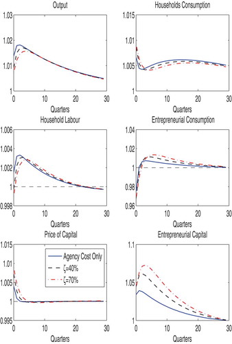
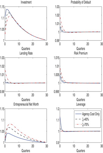
Figure 2. Impulse responses from a positive technology shock

Source: Author’s calculations

The positive productivity shock increases output, household consumption and net worth on impact. The increase in output and net worth results in an increased demand for capital which pushes the price of capital up. As the price of capital rises, the demand for investment falls which dampens the initial increase in output. As demand for investment falls, it boosts household consumption which in turn reduces household labour supply and dampens the increase in output. Though there is an increase in net worth, because the positive shock increases wages (including entrepreneurial wages) and rental income, the high price of capital makes the initial increase sluggish.

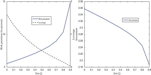
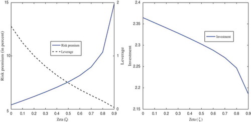
Figure 3. Relationship between expected leverage, expected risk premium, investment and limited enforcement in response to productivity shocks

Source: Author’s calculations

Increasing returns to entrepreneurial internal funds additionally increases net worth as the risk-neutral entrepreneur takes advantage of the rising price of capital by reducing their consumption. As the price of capital returns to its steady-state level, net worth attains it maximum before returning to the steady state. The increase in demand for investment and value of net worth leads to an increase in demand for external funds. This pushes up the default threshold and the probability of default on the impact of the shock. Following from the rise in the probability of default, the lending rate rises on the impact of the shock. Additionally, the increase in the value of internal funds, profit and the resulting increase in demand for external funds contributes to an increase in leverage.

The amplification effect of limited contract enforcement in the model is displayed by the three different lines corresponding to the different cases of contract enforceability. The growth in investment is dampened by limited enforcement. With a higher degree of limited enforcement, the risk premium and the probability of default are much more sensitive to increases in borrowing. As displayed in Figure 3, increases in the degree of limited enforcement ($\zeta )$ results in an increase in the risk premium and a decrease in leverage. Figure 3 also shows that the rate of investment falls with the degree of limited enforcement. Therefore, given a productivity shock, with a higher degree of limited enforcement, it is more difficult for entrepreneurs to use their net worth to expand investment (hence the lower growth in investment in Figure 2). Output responds to investment by displaying higher growth when the degree of limited enforcement is at its lowest level. When the degree of limited enforcement is at its highest level, the growth in output is at its lowest level. This reaction of aggregate output to the shock is consistent with the findings of Cooley et al. (2003) and Amaral and Quintin (2010). The negative effect of the limited enforcement on investment amplifies the increases in household consumption which in turn reduces household labour supply. The reduction in labour input is highest when the degree of limited enforcement is highest.

As limited enforcement worsens, the price of capital rises. This is as a result of the rise in the risk premium and a fall in the supply of capital resulting from the dampened growth in investment. As a result of this rise in the price of capital, both entrepreneurial capital and net worth increase the most when the degree of limited enforcement is highest. As earlier discussed, weak enforceability also exacerbates the effect of the shock on the probability of default, the lending rate and leverage. On impact of the shock, the probability of default rises by $2\mathrm{\%}$ when the degree of limited enforcement is $70\mathrm{\%}$ (i.e. when a firm can walk away with $70\mathrm{\%}$ of its output after default), $1\mathrm{\%}$ when the degree of limited enforcement is $40\mathrm{\%}$ (i.e. when a firm can walk away with $40\mathrm{\%}$ of its output after default) and $0.6\mathrm{\%}$ when there is “perfect” enforcement. The impact of the probability of default is reflected in the lending rate rising by $1.6\mathrm{\%}$, $0.5\mathrm{\%}$ and $0.2\mathrm{\%}$, respectively, when the degree of limited enforcement is $70\mathrm{\%}$, $40\mathrm{\%}$ and $0\mathrm{\%}$. As the lending rate and net worth increase following an increase in the degree of enforcement, external funding is reduced resulting in leverage being lowest when the degree of limited enforcement is highest.

2.3.2. Shocks to net worth

Figures 4 and 5 display the impulse responses to a shock to net worth, for three cases of limited enforcement (i.e. $\zeta =0\mathrm{\%}$ (perfect enforcement), $\zeta =40\mathrm{\%}$ (limited enforcement) and $\zeta =70\mathrm{\%}$ (imperfect enforcement)). This shock will be a one-time transfer of capital from entrepreneurs to households (lenders). The redistribution is $20\mathrm{\%}$ of the steady-state capital stock. This transfer increases household capital and reduces entrepreneurial net worth. This reduction in entrepreneurial net worth raises the demand for external financing and thus raising agency costs of investment. The decrease in net worth reduces investment which in turn decreases the supply of capital, therefore raising the equilibrium price of capital. This decrease in investment also leads to higher household consumption which serves as an incentive for households to decrease their labour input. The total impact is therefore a reduction in output. The decrease in value of net worth and demand for investment and the subsequent increase in demand for external funds increase the probability of default. Following the rise in the probability of default, the lending rate rises. Additionally, the fall in the value of internal funds leads to an increase in demand for external funds which in turn contributes to an increase in leverage.

The amplification effect of limited contract enforcement in the model is displayed by the three different lines corresponding to the different cases of contract enforceability. As earlier argued, higher degree of limited enforcement results in the risk premium and the probability of default being more sensitive to increases in borrowing. As displayed in Figure 6, increases in the degree of limited enforcement ($\zeta )$ results in an increase in the risk premium and a decrease in leverage.

Figure 4. Impulse responses from a negative shock to net worth

Source: Author’s calculations

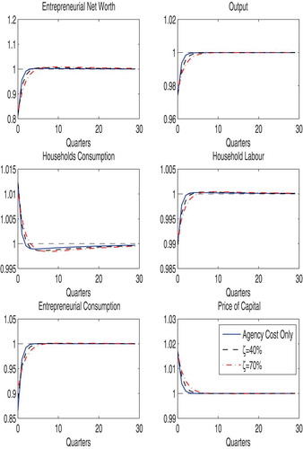
Figure 5. Impulse responses from a negative shock to net worth

Source: Author’s calculations

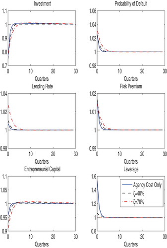
Figure 6 shows that the rate of investment falls with the degree of limited enforcement.

A one-time wealth transfer to households instantaneously reduces net worth. Therefore, given a higher $\zeta$, it is even much more difficult for entrepreneurs to use their net worth to expand investment (hence the lower growth in investment in Figure 5). The output is at its lowest when the degree of limited enforcement is at its highest level but highest when the degree of limited enforcement is lowest. The negative effect of the limited enforcement on investment further amplifies the increase in household consumption which in turn reduces household labour supply. The reduction in labour input is highest when the degree of limited enforcement is highest.

Figure 6. Relationship between expected leverage, expected risk premium, investment and limited enforcement in response to net worth shocks

Source: Author’s calculations

The negative impact of limited enforcement on both household labour supply and investment results in the effect of the shock on the output being equally amplified. The fall in net worth, investment and output results in entrepreneurial capital also falling and attaining its lowest level when the degree of limited enforcement is highest. As the degree of limited enforcement increases, the effect of the transfer on the probability of default, the lending rate and the degree of leverage is amplified. For instance, after the shock, the probability of default rises by $3.3\mathrm{\%}$ when the cost of enforcement is $70\mathrm{\%}$ (when a firm can walk away with $70\mathrm{\%}$ of its output after default), $2.5\mathrm{\%}$ when the cost of enforcement is $40\mathrm{\%}$ (i.e. when a firm can walk away with $40\mathrm{\%}$ of its output after default) and $2.5\mathrm{\%}$ when there is “perfect” enforcement.⁶ The impact of the probability of default is reflected in the lending rate rising by $3\mathrm{\%}$, $1.1\mathrm{\%}$ and $0.7\mathrm{\%}$, respectively, when the degree of limited enforcement is $70\mathrm{\%}$, $40\mathrm{\%}$ and $0\mathrm{\%}$. As lending rate increases and net worth decreases following an increase in the degree of limited enforcement, external funding is reduced resulting in the degree of leverage being lowest when the degree of limited enforcement is highest.

2.3.3. Sensitivity analysis: limited enforcement, output and net worth

In Table 2, following a positive productivity shock, an increase in the degree of limited enforcement, from $0\mathrm{\%}$ to $40\mathrm{\%}$, is associated with a decrease in output volatility from $2.37\mathrm{\%}$ to $2.20\mathrm{\%}$ whilst an increase in the degree of limited enforcement from $0\mathrm{\%}$ to $70\mathrm{\%}$, is associated with a decrease in output volatility from $2.37\mathrm{\%}$ to $2.05\mathrm{\%}$. Similarly, expected output decreases as the degree of limited enforcement increases. In contrast, we find that as the degree of limited enforcement increases, expected net worth and its volatility follow similar trends. In a similar vein, expected lending rate and its volatility increase with the degree of limited enforcement. Our results are consistent with other studies (Cooley et al., 2003; Quintin, 2000) which made similar findings on the impact of limited contract enforcement on output.

Table 1. Calibration

Description	Parameter	Value
Contract Enforcement	$\zeta$	(0,1)
Verification Cost	$\mu$	0.15
Discount Factor	$\beta$	0.99
Labour Supply Disutility	$\nu$	2.52
Productivity Parameter	$A$	1.00
Persistence in Aggregate Technology Shock	${\rho }_A$	0.95
Depreciation Rate of Capital	$\delta$	$2\mathrm{\%}$
Share of Capital in Production	${\alpha }_K$	$36\mathrm{\%}$
Share of Entrepreneurial Labour in Production	${\alpha }_e$	$0.01\mathrm{\%}$
Share of Household Labour in Production	${\alpha }_H$	$63.99\mathrm{\%}$
Additional Discount Rate for Entrepreneurs	$\gamma$	$91\mathrm{\%}$
Fraction of Entrepreneurs	$\eta$	$10\mathrm{\%}$
Standard Deviation of $\mathrm{\Phi }(\omega )$	${\sigma }_{\omega }$	$20.7\mathrm{\%}$
Standard Deviation of Net Worth Shock	${\sigma }_n$	$10\mathrm{\%}$
Standard Deviation of Aggregate Productivity Shock

Table 2. Productivity shock

Cost of Enforcement	$0\mathrm{\%}$	$40\mathrm{\%}$	$70\mathrm{\%}$	$0\mathrm{\%}$	$40\mathrm{\%}$	$70\mathrm{\%}$
Statistic	Mean			Volatility
Output	1.01	1.00	0.99	$2.37\mathrm{\%}$	$2.20\mathrm{\%}$	$2.05\mathrm{\%}$
Net Worth	0.91	1.41	1.80	$7.10\mathrm{\%}$	$10.36\mathrm{\%}$	$12.44\mathrm{\%}$
Lending Rate	$0.47\mathrm{\%}$	$1.36\mathrm{\%}$	$6.22\mathrm{\%}$	$0.11\mathrm{\%}$	$0.30\mathrm{\%}$	$1.16\mathrm{\%}$

We measure volatility by standard deviations expressed in percentages.

Table 3 presents our findings following a one-time wealth transfer from entrepreneurs to households (lenders). One interesting finding in the data is that countries with more limited contract enforcement tend to exhibit more volatility in output. The result from our model with one-time wealth transfer is able to reproduce this observation. Whist expected output decreases, the volatility of output increases as the degree of limited enforcement increases. Similarly, both expected net worth and its volatility increase as the degree of limited enforcement increases. The preceding outcome is not different in terms of the lending rate. Expected lending rate and its volatility increase as the degree of limited enforcement rises.

Table 3. One-time wealth transfer

Cost of Enforcement	$0\mathrm{\%}$	$40\mathrm{\%}$	$70\mathrm{\%}$	$0\mathrm{\%}$	$40\mathrm{\%}$	$70\mathrm{\%}$
Statistic	Mean			Volatility
Output	1.01	1.00	0.99	$2.28\mathrm{\%}$	$2.32\mathrm{\%}$	$2.19\mathrm{\%}$
Net Worth	0.91	1.41	1.80	$18.49\mathrm{\%}$	$18.46\mathrm{\%}$	$18.92\mathrm{\%}$
Lending Rate	$0.47\mathrm{\%}$	$1.36\mathrm{\%}$	$6.22$	$0.36\mathrm{\%}$	$0.62\mathrm{\%}$	$1.87\mathrm{\%}$

We measure volatility by standard deviations expressed in percentages.

This result may be seen as being especially pertinent for the case of small firms that use their net worth as collateral and rely largely on external finance for production. As contract enforcement weakens from $0\mathrm{\%}$ to $40\mathrm{\%}$ and from $0\mathrm{\%}$ to $70\mathrm{\%}$ (Tables 2 and 3), the lending rate increases by $189.3\mathrm{\%}$ and $1,223.4\mathrm{\%}$, respectively. This suggests entrants and smaller firms are credit constrained and find the cost of investment high. As a consequence, the growth of such firms as well as the growth of the overall economy is impeded (Albuquerque & Hopenhayn, 2000; Amaral & Quintin, 2010).

2.3.4. Sensitivity analysis: welfare consequences of limited contract enforcement

A very important issue worth commenting on is the effect of limited enforcement on household welfare, the presumption being that weaker enforcement reduces welfare. Following Lucas (1987), we estimate welfare loss (consumption equivalent) as the percentage decrease in household consumption in the economy with perfect enforcement which makes households indifferent between the economy with limited enforcement and the economy with perfect enforcement (Appendix 4.5). In the context of the present model, when enforceability is poor, investment responds positively. In light of this, in response to a positive productivity shock, household consumption increases which results in household labour supply falling. This leads to household welfare increasing accordingly. However, the initial increase in welfare is dampened when enforcement worsens. The result displayed in Table 4 provides an additional support for the effect of limited enforcement on household welfare when there is a positive productivity shock. The result shows that as the degree of limited enforcement increases from $40\mathrm{\%}$ to $70\mathrm{\%}$, the average household consumption equivalent welfare loss increases from $0.86\mathrm{\%}$ to $1.84\mathrm{\%}$.

Table 4. Welfare loss

Cost of Enforcement	40%	$70\mathrm{\%}$	$40\mathrm{\%}$	$70\mathrm{\%}$
Statistic	Productivity Shock		Wealth Transfer
Consumption Equivalent of Welfare Loss	0.86%	1.84%	0.9%	1.89%

Welfare consequences of productivity shock and one-time wealth transfer

In response to a one-time transfer of wealth from entrepreneurs to households, consumption of the latter increases which then results in labour supply falling. This leads to household welfare increasing, on the impact of the shock. However, as the transfer is one-time the initial increase in welfare is short-lived. Table 4 presents the results of the impact of the wealth transfer on households. We show that as the degree of limited enforcement increases from $40\mathrm{\%}$ to $70\mathrm{\%}$, the average consumption equivalent welfare loss increases from $0.9\mathrm{\%}$ to $1.89\mathrm{\%}$.

2.3.5. Limited enforcement, monitoring cost and output

Table 5 displays the effect of changes in monitoring cost and the degree of limited enforcement on output.

Table 5. Effect of limited enforcement and monitoring cost on output

	Monitoring and Verification Cost
	$\mu =5$	$\mu =10\mathrm{\%}$	$\mu =15\mathrm{\%}$	$\mu =20\mathrm{\%}$	$\mu =25\mathrm{\%}$
Degree of Enforcement	Percentage Change in Output
$\zeta =0\mathrm{\%}$	$1.82\mathrm{\%}$	$1.71\mathrm{\%}$	$1.66\mathrm{\%}$	$1.62\mathrm{\%}$	$1.59\mathrm{\%}$
$\zeta =40\mathrm{\%}$	$0.90\mathrm{\%}$	$0.89\mathrm{\%}$	$0.88\mathrm{\%}$	$0.88\mathrm{\%}$	$0.86\mathrm{\%}$
$\zeta =70\mathrm{\%}$	$-0.42\mathrm{\%}$	$-0.19\mathrm{\%}$	$-0.10\mathrm{\%}$	$-0.04\mathrm{\%}$	$0.00\mathrm{\%}$

Smaller $\mu$ means better credit information. Smaller $\zeta$ means better contract enforcement.

Percentage change in output relative to the steady-state output when $\zeta =70\mathrm{\%}$

It is observed that as monitoring cost fall (i.e. as credit information improves), its effect on output increases. Similarly, as enforcement improves, its impact on output increases. This finding is consistent with the empirical result (Cooley et al., 2003; Steinberg, 2013), particularly, where we establish that both poor depth of credit information and limited enforcement have a negative effect on output.

3. Concluding remarks

This study presents a dynamic stochastic general equilibrium model of asymmetric information and limited contract enforcement in financial markets. The first of these features—a fairly standard way of incorporating capital market frictions into macroeconomic models is reflected in the idea of costly state verification by financial intermediaries. The second feature—a much less standard way of capturing such frictions—is reflected in the notion of institutional weaknesses in holding defaulters to account. It is this second aspect on which our interest has been focused and in which the contribution of the analysis is mainly found. The findings have shown how limited contract enforcement may affect fluctuations in key macroeconomic variables such as output, employment and investment through its impact on key financial variables such as interest rates, risk premium, default risk and leverage. Furthermore, the findings have shown that lower level of output with an accompanying higher output volatility characterises weakly enforced financial contracts. The findings also show the phenomenon has negative consequences for firm growth and welfare to the society. These findings are particularly relevant for developing countries, where institutions are often weak, fragile and fragmented because of poor quality of governance and further suggest that improving such quality has the potential to improve the prospects of such countries.

Additional information

Funding

The author received no direct funding for this research.

Notes on contributors

Adams Sorekuong Yakubu Adama

Adams Sorekuong Yakubu Adama is an Assistant Professor at the School of Economics, University of Cape Coast, Ghana. He holds a PhD in Economics from the University of Manchester, UK. His research interest includes: Small firm financing and growth, institutional quality and development especially in emerging economies where such institutions are weak and fragile, Macroeconomic policy issues and dynamic stochastic general equilibrium (DSGE) modelling. My current work is focusing on how institutional weakness vis-à-vis limited contract enforcement is affecting African firms. Adama is an ad hoc reviewer for Reviewer for Development Studies Research.

Notes

1. That is to say bad enforcement results in self-financing of production and on a small scale.

2. In the general equilibrium setting, risk-averse households are the source of loanable funds to entrepreneurs. However, in terms of the financial contract, they will be effectively risk neutral because (1) there will be no aggregate uncertainty over the duration of the contract and (2) households can diversify away all idiosyncratic risk.

3. See Appendix (4.4) for detailed derivation.

4. See Appendix (4.1) for detailed derivation.

5. In the earlier working paper version of their paper, Carlstrom and Fuerst (1997) assumed that a constant fraction of the entrepreneurs died each period, and sold their accumulated capital stock to households. In terms of consumption, this is equivalent to assuming that the entrepreneurs consume a constant fraction of their capital holdings each period.

6. In the second quarter, for instance, the probability of default is 1.9%, 1% and 0.6% when the cost of enforcement is 70%, 40% and 0%, respectively.

Appendix A

4.1 Household Optimisation Problem

Households maximise expected lifetime utility

${\mathbb{E}}_0\left[\sum _{t=0}^{\mathrm{\infty }}{\beta }^{t}U(c_t,(1-L_t))\right]$

subject to

$c_t+q_t\left[k_{t+1}^h-(1-\delta )k_t^h\right]=w_t{L}_t+r_t{k}_t^h$

where $U(c_t,(1-L_t))=ln(c_t)+\nu (1-L_t)$

Lagrange for the problem:

$\mathcal{L}={\mathbb{E}}_0\left[\sum _{t=0}^{\mathrm{\infty }}{\beta }^t\left[ln(c_t)+\nu (1-L_t)\right]\right]+{\mathbb{E}}_0\left[\sum _{t=0}^{\mathrm{\infty }}{\beta }^t\left[{\lambda }_t\left(w_t{L}_t+r_t{k}_t^h-c_t-q_t(k_{t+1}^h-(1-\delta )k_t^h)\right)\right]\right]$

First Order Conditions from household maximisation problem:

(11) $c:U_c(c_t,1-L_t)-{\lambda }_t=0$(11)

(12) $k_{t+1}^h:-q_t{\lambda }_t+\beta {\mathbb{E}}_t\left[{\lambda }_{t+1}\left(r_{t+1}+q_{t+1}(1-\delta )\right)\right]=0$(12)

(13) $L:U_L(c_t,1-L_t)+{\lambda }_t{w}_t=0$(13)

Equation (13)(13) $L:U_L(c_t,1-L_t)+{\lambda }_t{w}_t=0$(13) implies ${\lambda }_t=\frac{\nu }{W_t}$

Note that $U_c(c_t,1-L_t)=c_t^{-1}$; $U_L(c_t,1-L_t)=-\nu$. Then

(14) $w_t=\frac{U_L(c_t,1-L_t)}{U_c(c_t,1-L_t)}=\frac{\nu }{c_t^{-1}}$(14)

Equation (14)(14) $w_t=\frac{U_L(c_t,1-L_t)}{U_c(c_t,1-L_t)}=\frac{\nu }{c_t^{-1}}$(14) implies:

$c_t={\left(\frac{\nu }{w_t}\right)}^{-1}=\left(\frac{w_t}{\nu }\right)$

Using Equations (11)(11) $c:U_c(c_t,1-L_t)-{\lambda }_t=0$(11) and (12(12) $k_{t+1}^h:-q_t{\lambda }_t+\beta {\mathbb{E}}_t\left[{\lambda }_{t+1}\left(r_{t+1}+q_{t+1}(1-\delta )\right)\right]=0$(12) ) we can write the Euler Equation as:

(15) $q_t{U}_c(c_t,1-L_t)=\beta {\mathbb{E}}_t\left[U_c(c_{t+1},1-L_{t+1})\left(r_{t+1}+q_{t+1}(1-\delta )\right)\right]$(15)

Equation (15)(15) $q_t{U}_c(c_t,1-L_t)=\beta {\mathbb{E}}_t\left[U_c(c_{t+1},1-L_{t+1})\left(r_{t+1}+q_{t+1}(1-\delta )\right)\right]$(15) is then simplified as:

$q_t{c}_t^{-1}=\beta {\mathbb{E}}_t\left[c_{t+1}^{-1}\left(r_{t+1}+q_{t+1}(1-\delta )\right)\right]$

4.2 Consumption-good Producing Firms

We specify the production function as:

$Y_t=A_t{K}_t^{{\alpha }_K}{H}_t^{{\alpha }_H}{H}_t^{e{\alpha }_e}$

Perfect competition in factor markets implies the following factor prices:

$r_t=A_t{F}_1(K_t,H_t,H_t^e)={\alpha }_K{A}_t{K}_t^{{\alpha }_K-1}{H}_t^{{\alpha }_H}{H}_t^{e{\alpha }_e}=\frac{Y_t}{K_t}$

$w_t=A_t{F}_2(K_t,H_t,H_t^e)={\alpha }_H{A}_t{K}_t^{{\alpha }_K}{H}_t^{{\alpha }_H-1}{H}_t^{e{\alpha }_e}=\frac{Y_t}{H_t}$

$w_t^e=A_t{F}_3(K_t,H_t,H_t^e)={\alpha }_e{A}_t{K}_t^{{\alpha }_K}{H}_t^{{\alpha }_H}{H}_t^{e{\alpha }_e-1}=\frac{Y_t}{H_t^e}$

4.3 The Entrepreneur

Entrepreneurs maximise their expected lifetime utility

(16) ${\mathbb{E}}_0\left[\sum _{t=0}^{\mathrm{\infty }}{(\beta \gamma )}^t{c}_t^e\right]$(16)

subject to

(17) $K_{t+1}^e=\left(\eta w_t^e+K_t^e\left[q_t(1-\delta )+r_t\right]\right)\frac{f(\bar{\omega }(q_t))}{1-q_{t}g(\bar{\omega }(q_t))}-\frac{c_t^e}{q_t}$(17)

Lagrange for the problem:

$\mathcal{L}={\mathbb{E}}_0\sum _{t=0}^{\mathrm{\infty }}{\beta }^t(c_t^e)+{\mathbb{E}}_0\sum _{t=0}^{\mathrm{\infty }}{\beta }^t\left[{\lambda }_t\left(\left(\eta w_t^e+K_t^e\left[q_t(1-\delta )+r_t\right]\right)\frac{f(\bar{\omega }(q_t))}{1-q_{t}g(\bar{\omega }(q_t))}-\frac{c_t^e}{q_t}-K_{t+1}^e\right)\right]$

$c_t^e:u_{{ }^{c^e}}(t)-{\lambda }_t/q_t=0$

${\lambda }_t=q_t$

$K_{t+1}^e:-{\lambda }_t+(\beta \gamma ){\mathbb{E}}_t\{{\lambda }_{t+1}(q_{t+1}(1-\delta )+r_{t+1})\frac{f(\bar{\omega }(q_{t+1}))}{(1-q_{t+1}g(\bar{\omega }(q_{t+1})))}\}=0$

(18) $q_t=(\beta \gamma ){\mathbb{E}}_t\left[(q_{t+1}(1-\delta )+r_{t+1})\frac{q_{t+1}f(\bar{\omega }(q_{t+1}))}{(1-q_{t+1}g(\bar{\omega }(q_{t+1})))}\right]$(18)

4.4 Optimal contract

The optimal contract is given by the pair $(i,\bar{\omega })$ (taking as given net worth $n$ and capital price $q)$ which solves:

$\underset{i,\bar{\omega }}{max}qif(\bar{\omega })$

subject to

$qig(\bar{\omega })\ge i-n{\mathrm{L}\mathrm{e}\mathrm{n}\mathrm{d}\mathrm{e}\mathrm{r}}^{\prime }\mathrm{s}\mathrm{P}\mathrm{a}\mathrm{r}\mathrm{t}\mathrm{i}\mathrm{c}\mathrm{i}\mathrm{p}\mathrm{a}\mathrm{t}\mathrm{i}\mathrm{o}\mathrm{n}\mathrm{c}\mathrm{o}\mathrm{n}\mathrm{s}\mathrm{t}\mathrm{r}\mathrm{a}\mathrm{i}\mathrm{n}\mathrm{t}$

$qif(\bar{\omega })\ge n{\mathrm{E}\mathrm{n}\mathrm{t}\mathrm{r}\mathrm{e}\mathrm{p}\mathrm{r}\mathrm{e}\mathrm{n}\mathrm{e}\mathrm{u}\mathrm{r}}^{\prime }\mathrm{s}\mathrm{P}\mathrm{a}\mathrm{r}\mathrm{t}\mathrm{i}\mathrm{c}\mathrm{i}\mathrm{p}\mathrm{a}\mathrm{t}\mathrm{i}\mathrm{o}\mathrm{n}\mathrm{c}\mathrm{o}\mathrm{n}\mathrm{s}\mathrm{t}\mathrm{r}\mathrm{a}\mathrm{i}\mathrm{n}\mathrm{t},\mathrm{a}\mathrm{l}\mathrm{w}\mathrm{a}\mathrm{y}\mathrm{s}\mathrm{s}\mathrm{a}\mathrm{t}\mathrm{i}\mathrm{s}\mathrm{f}\mathrm{i}\mathrm{e}\mathrm{d}$

Technically, only the first constraint binds.

Lagrangian for this problem:

$\mathcal{L}=qif(\bar{\omega })+\lambda \left[qig(\bar{\omega })-i+n\right]$

The First Order Conditions:

(19) $\frac{\mathrm{\partial }\mathcal{L}}{\mathrm{\partial }i}=qf(\bar{\omega })+\lambda \left[qg(\bar{\omega })-1\right]=0$(19)

(20) $\frac{\mathrm{\partial }\mathcal{L}}{\mathrm{\partial }\bar{\omega }}=qi{f}^{\prime }(\bar{\omega })+\lambda qi{g}^{\prime }(\bar{\omega })=0$(20)

(21) $\frac{\mathrm{\partial }\mathcal{L}}{\mathrm{\partial }\lambda }=qig(\bar{\omega })-i+n=0$(21)

Re-arranging Equation (19)(19) $\frac{\mathrm{\partial }\mathcal{L}}{\mathrm{\partial }i}=qf(\bar{\omega })+\lambda \left[qg(\bar{\omega })-1\right]=0$(19) :

$q\left[\frac{1}{\lambda }f(\bar{\omega })+g(\bar{\omega })\right]=1$

$\lambda =-\frac{f^{\prime }(\bar{\omega })}{g^{\prime }(\bar{\omega })}$

Then, re-arranging Equation (20)(20) $\frac{\mathrm{\partial }\mathcal{L}}{\mathrm{\partial }\bar{\omega }}=qi{f}^{\prime }(\bar{\omega })+\lambda qi{g}^{\prime }(\bar{\omega })=0$(20) , we get

$\frac{1}{\lambda }=\frac{g^{\prime }(\bar{\omega })}{-f^{\prime }(\bar{\omega })}=\frac{(1-\zeta )(1-\mathrm{\Phi }(\bar{\omega }))-\mu \varphi (\bar{\omega })}{(1-\zeta )(1-\mathrm{\Phi }(\bar{\omega }))}=1-\frac{\mu \varphi (\bar{\omega })}{(1-\zeta )(1-\mathrm{\Phi }(\bar{\omega }))}$

Then, combined with Equation (6)(6) $f(\bar{\omega })+g(\bar{\omega })=1-\mu \mathrm{\Phi }(\bar{\omega })$(6) , we have the following condition:

(22) $q\left[1-\mu \mathrm{\Phi }(\bar{\omega })-\frac{\mu \varphi (\bar{\omega })f(\bar{\omega })}{(1-\zeta )(1-\mathrm{\Phi }(\bar{\omega }))}\right]=1$(22)

This can also be written as:

$q\left[1-\mu \mathrm{\Phi }(\bar{\omega })+\mu \varphi (\bar{\omega })\frac{f(\bar{\omega })}{f^{\prime }(\bar{\omega })}\right]=1$

4.5 Consumption Equivalent Welfare Loss

Let $\lambda$ denote consumption equivalent welfare loss, the fraction of consumption one would be willing to give up each period in the economy with perfect enforcement.

$\mathbb{E}(V_t^{\mathbf{p}\mathbf{e}\mathbf{r}\mathbf{f}\mathbf{e}\mathbf{c}\mathbf{t}\mathbf{e}\mathbf{n}\mathbf{f}\mathbf{o}\mathbf{r}\mathbf{c}\mathbf{e}\mathbf{m}\mathbf{e}\mathbf{n}\mathbf{t}}(\lambda ))=\mathbb{E}\left[\left(ln(c_t(1+\lambda ))+\nu (1-L_t)\right)+\beta {\mathbb{E}}_t\left[V_{t+1}^{\mathbf{p}\mathbf{e}\mathbf{r}\mathbf{f}\mathbf{e}\mathbf{c}\mathbf{t}\mathbf{e}\mathbf{n}\mathbf{f}\mathbf{o}\mathbf{r}\mathbf{c}\mathbf{e}\mathbf{m}\mathbf{e}\mathbf{n}\mathbf{t}}\right]\right]$

$\lambda$ shows up every period and we assume it is deterministic and this reduces to:

$\mathbb{E}(V_t^{\mathbf{p}\mathbf{e}\mathbf{r}\mathbf{f}\mathbf{e}\mathbf{c}\mathbf{t}\mathbf{e}\mathbf{n}\mathbf{f}\mathbf{o}\mathbf{r}\mathbf{c}\mathbf{e}\mathbf{m}\mathbf{e}\mathbf{n}\mathbf{t}}(\lambda ))=\frac{1}{1-\beta }(1+\lambda )+$

$\mathbb{E}\left[\left(ln(c_t)+\nu (1-L_t)\right)+\beta {\mathbb{E}}_t\left[V_{t+1}^{\mathbf{p}\mathbf{e}\mathbf{r}\mathbf{f}\mathbf{e}\mathbf{c}\mathbf{t}\mathbf{e}\mathbf{n}\mathbf{f}\mathbf{o}\mathbf{r}\mathbf{c}\mathbf{e}\mathbf{m}\mathbf{e}\mathbf{n}\mathbf{t}}\right]\right]$

The term in brackets is then:

$\mathbb{E}(V_t^{\mathbf{p}\mathbf{e}\mathbf{r}\mathbf{f}\mathbf{e}\mathbf{c}\mathbf{t}\mathbf{e}\mathbf{n}\mathbf{f}\mathbf{o}\mathbf{r}\mathbf{c}\mathbf{e}\mathbf{m}\mathbf{e}\mathbf{n}\mathbf{t}}(\lambda ))=\frac{1}{1-\beta }(1+\lambda )+\mathbb{E}(V_t^{\mathbf{p}\mathbf{e}\mathbf{r}\mathbf{f}\mathbf{e}\mathbf{c}\mathbf{t}\mathbf{e}\mathbf{n}\mathbf{f}\mathbf{o}\mathbf{r}\mathbf{c}\mathbf{e}\mathbf{m}\mathbf{e}\mathbf{n}\mathbf{t}})$

Then, we want to find the $\lambda$ that equates this with expected welfare in an economy with limited enforcement. We have:

$\mathbb{E}(V_t^{\mathbf{p}\mathbf{e}\mathbf{r}\mathbf{f}\mathbf{e}\mathbf{c}\mathbf{t}\mathbf{e}\mathbf{n}\mathbf{f}\mathbf{o}\mathbf{r}\mathbf{c}\mathbf{e}\mathbf{m}\mathbf{e}\mathbf{n}\mathbf{t}}(\lambda ))=\mathbb{E}(V_t^{\mathbf{l}\mathbf{i}\mathbf{m}\mathbf{i}\mathbf{t}\mathbf{e}\mathbf{d}\mathbf{e}\mathbf{n}\mathbf{f}\mathbf{o}\mathbf{r}\mathbf{c}\mathbf{e}\mathbf{m}\mathbf{e}\mathbf{n}\mathbf{t}})$

Or

$\frac{1}{1-\beta }(1+\lambda )+\mathbb{E}(V_t^{\mathbf{p}\mathbf{e}\mathbf{r}\mathbf{f}\mathbf{e}\mathbf{c}\mathbf{t}\mathbf{e}\mathbf{n}\mathbf{f}\mathbf{o}\mathbf{r}\mathbf{c}\mathbf{e}\mathbf{m}\mathbf{e}\mathbf{n}\mathbf{t}})=\mathbb{E}(V_t^{\mathbf{l}\mathbf{i}\mathbf{m}\mathbf{i}\mathbf{t}\mathbf{e}\mathbf{d}\mathbf{e}\mathbf{n}\mathbf{f}\mathbf{o}\mathbf{r}\mathbf{c}\mathbf{e}\mathbf{m}\mathbf{e}\mathbf{n}\mathbf{t}})$

Then

$\lambda =exp\left[(1-\beta )\times (\mathbb{E}(V_t^{\mathrm{l}\mathrm{i}\mathrm{m}\mathrm{i}\mathrm{t}\mathrm{e}\mathrm{d}\mathrm{e}\mathrm{n}\mathrm{f}\mathrm{o}\mathrm{r}\mathrm{c}\mathrm{e}\mathrm{m}\mathrm{e}\mathrm{n}\mathrm{t}})-\mathbb{E}(V_t^{\mathrm{p}\mathrm{e}\mathrm{r}\mathrm{f}\mathrm{e}\mathrm{c}\mathrm{t}\mathrm{e}\mathrm{n}\mathrm{f}\mathrm{o}\mathrm{r}\mathrm{c}\mathrm{e}\mathrm{m}\mathrm{e}\mathrm{n}\mathrm{t}}))\right]-1$

If we take the economy with perfect enforcement to have higher welfare, then $\lambda <0$. This means you would be willing to give up consumption in the high welfare economy to have the same welfare as an economy with lower welfare (limited enforcement).

References

- Albuquerque, R., & Hopenhayn, H. (2000). Optimal dynamic lending contracts with imperfect enforceability. In Afa 2001 new orleans meetings (pp. 00–24). Berkeley, CA.
- Amaral, P. S., & Quintin, E. (2010). Limited enforcement, financial intermediation, and economic development: A quantitative assessment. International Economic Review, 51(3), 785–811. doi:10.1111/iere.2010.51.issue-3
- Bernanke, B. S., Gertler, M., & Gilchrist, S. (1999). The financial accelerator in a quantitative business cycle framework. In J. B. Taylor & M. Woodford (Eds.). Handbook of macroeconomics (Vol. 1 Part C, pp. 1341–1393). Amsterdam, The Netherlands: Elsevier.
- Boedo, H. J. M., Senkal, A., & D’Erasmo, P. (2011). Misallocation, informality and human capital. In 2011 meeting papers (pp. 881), Society for Economic Dynamics. Ghent, Belgium.
- Carlstrom, C. T., & Fuerst, T. S. (1997). Agency costs, net worth, and business fluctuations: A computable general equilibrium analysis. The American Economic Review, 87(5), 893–910.
- Carlstrom, C. T., & Fuerst, T. S. (1998). Agency costs and business cycles. Economic Theory, 12(3), 583–597. doi:10.1007/s001990050236
- Carlstrom, C. T., & Fuerst, T. S. (2001). Monetary shocks, agency costs, and business cycles. Carnegie-Rochester Conference Series on Public Policy, 54(1), 29–35.
- Carlstrom, C. T., Fuerst, T. S., & Paustian, M. (2010). Optimal monetary policy in a model with agency costs. Journal of Money, Credit and Banking, 42(s1), 37–70. doi:10.1111/jmcb.2010.42.issue-s1
- Castro, R., Clementi, G. L., & MacDonald, G. (2004). Investor protection, optimal incentives, and economic growth. The Quarterly Journal of Economics, 119(3), 1131–1175. doi:10.1162/0033553041502171
- Cooley, T., Marimon, R., & Quadrini, V. (2003). Aggregate consequences of limited contract enforceability. (Tech. Rep.). National Bureau of Economic Research. Massachusetts, USA.
- De Fiore, F., Teles, P., & Tristani, O. (2011). Monetary policy and the financing of firms. American Economic Journal: Macroeconomics, 3(4), 112–142.
- Gertler, M. (1988). Financial structure and aggregate economic activity: An overview. Journal of Money, Credit, and Banking, 20(3). doi:10.2307/1992535
- Gertler, M., & Bernanke, B. (1989). Agency costs, net worth and business fluctuations. In F. Kydland (Ed.), Business cycle theory. London: Edward Elgar Publishing Ltd.
- Khan, A., & Ravikumar, B. (2001). Growth and risk-sharing with private information. Journal of Monetary Economics, 47(3), 499–521. doi:10.1016/S0304-3932(01)00053-8
- Levin, A. T., Natalucci, F. M., & Zakrajsek, E. (2004). The magnitude and cyclical behavior of financial market frictions. Washington, DC.
- Levine, R., Loayza, N., & Beck, T. (2000). Financial intermediation and growth: Causality and causes. Journal of Monetary Economics, 46(1), 31–77. doi:10.1016/S0304-3932(00)00017-9
- Lucas, R. E. (1987). Models of business cycles (Vol. 26). Oxford: Basil Blackwell.
- Marcet, A., & Marimon, R. (1992). Communication, commitment, and growth. Journal of Economic Theory, 58(2), 219–249. doi:10.1016/0022-0531(92)90054-L
- Quintin, E. (2000). Limited enforcement and the organization of production. Unpublished manuscript. Federal Reserve Bank of Dallas. Texas, USA.
- Steinberg, J. B. (2013). Information, contract enforcement, and misallocation.Mimeo, 1. Minnesota, USA: University of Minnesota.