Mapping of sovereign risks in small island economies: An application of contingent claim approach to fiji

Abstract

While a decline in the market value of sovereign assets (below a benchmark level of liabilities) can trigger sovereign distress/default risk, volatility in sovereign assets can increase the risk premium on domestic debt and credit spread on external debt. These can escalate the probability of debt default. Therefore, measuring the probability and distance to debt distress associated with sovereign positions is important for assessing the macro-financial risks of an aggregate economy. This paper presents an application of the Contingent Claim Approach (CCA) for measuring the implied asset value and its volatility for the case of Fiji. The CCA captures non-linear changes to sovereign assets and liabilities that are hardly captured by other macroeconomic variables. Our consistent empirical findings indicate no sovereign debt distress for Fiji. Unavailability of partial data on the certain composition of sovereign assets and liabilities is a limitation, but our results are consistent and useful guide to debt policy in Fiji. It is also useful for future research on debt sustainability in other similar smaller developing economies.

Keywords:

• Sovereign risk
• contingent claim approach
• macro-financial risk analysis
• south pacific
• Fiji

Jel:

• F31
• F32
• E52
• F4

PUBLIC INTEREST STATEMENT

Sovereign liabilities (Government and Monetary Authority combined) are promised payments on the debts against the uncertain market value of sovereign assets. A decline in the value of assets below a certain level of promised payments can trigger sovereign distress or default. This paper employs the Contingent Claim Approach to assess the sustainability of Government debt in a small economy (Fiji) by analyzing the distance to debt distress and the probability of default. It finds that despite the internal-external shocks, Fiji has low levels of debt stress and between 2%-3% probability of default.

1. Introduction

Traditional analysis of sovereign debt based on vulnerability indices and macro fundamentals do not adequately capture the non-linear changes to sovereign assets and liabilities. Macro-financial risk assessment based on Contingent Claim Analysis (CCA) adequately supplements the overall macro-financial risk assessment of an aggregate economy because CCA assesses the evaluation of uncertainty in the future value of sovereign assets related to sovereign liabilities, where option pricing is used to construct risk-adjusted balance sheet factoring market information.

The core of CCA is to consider sovereign liabilities as contingent claims¹ on sovereign assets whose valuations are uncertain. This uncertainty is calculated by a probability distribution along a time horizon. It derives the implied value of sovereign assets and their volatility from the market value of liabilities to establish sovereign sustainability. Therefore, it is a method of embedding financial market developments with accounting information to deal with market imperfections. The CCA applied to a national balance sheet can effectively analyze the value of assets and liabilities based on the uncertain value of assets, risk transmission between alternative sectors and risk exposure subdued within the national balance sheet. The volatility in sovereign assets increases the risk premium on domestic debt and credit spread on international bonds. Therefore, this paper discusses various aspects of sovereign risks of Fiji to help manage foreign debt and attract sustainable capital inflows to support national economic development.

The South Pacific region consists of about a dozen small island states with all having “population penalty²” syndrome unhealthy for scale-effects. Additionally, there are other challenges (dependence on foreign aid and foreign-capital, capacity constraints, and lack of adequate resources, primitive technology, small domestic market, and greater vulnerability to climate-related events). Further, a small domestic/external friction can create a big impact on the macro-financial health of such economies. As such, assessing the macro-financial risks are important for such economies who have limited capacity to mitigate large shocks to their incomes and welfare. The proposed work in this paper is a pioneering attempt to study CCA using the Balance Sheet Framework for Fiji. Although it is primarily based on Gray, Merton, and Bodie (2009) method, with few modifications being introduced to contextualize the analysis. These are (i) equity (base money and other local currency debt) is used as one-composite variable (ii) historical spot-rate is used instead of the forward rate due to lack of data.

This paper is organized as follows. The following briefly introduces the Pacific context and the Fijian economy. The next section surveys prominent works on the CCA with important models based on this are discussed in section 4. The conceptual framework of the paper is presented in Section 5. Model specification, variable definitions, and the empirical results for Fiji’s sovereign sector balance sheet analysis are in sections 7 and 8, respectively. The final section 8 concludes.

2. Macro-financials of the Fiji economy

Fiji is an emerging, open economy. Since 2008, Fiji has recorded an average economic growth rate of 3% (IMF, 2019-October)³ while the growth of per capita income has been modest to average just over 1% per annum. Fiji has sustained many shocks such as trade boost (1989), devaluation (1988, 1998 & 2009), political crises (1987, 2000 & 2006) and fuel price hikes (various years) and tropical cyclones & flash-flooding (once every year). The impact of these events has been significant. So far, the implications have not been analyzed using the BSA framework for Fiji or for the Pacific region. There are several reasons for selecting Fiji. First, it is perhaps the best economy of the region which is fast emerging to be an upper-middle-income country. Second, most financial crises have impacted countries where financial markets were not well developed. Third, Fiji remains dependent on external debt (government) and domestic debt (private) financing. Finally, since financial risks are not evenly distributed across economic sectors, the Fijian economy is a good case study for small and vulnerable economies. However, before we go into details, it is important to review the past monetary and fiscal policy responses to various shocks.

In the period 1970–2007, the first major reform (after independence in 1970) was the pegging of the Fiji dollar with USD in 1974. Earlier it was pegged with the British Pound. The Fiji Dollar was pegged against a basket of currencies (based on major trading partners) in 1975. The monetary function was managed by then the Central Monetary Authority, until the formation of Reserve Bank of Fiji (RBF) in 1984. Initially, the RBF had been using direct quantitative policy, until 1988 (Jayaraman & Choong, 2008) when the first major devaluation of the Fiji Dollar (by 33%) was announced in 1988. Under a fixed exchange rate regime, monetary authority usually practices devaluation of the currency to absorb serious shocks that may impact the level of foreign reserves. Subsequently, large-scale financial sector reforms were undertaken in 1989 in order to ease lending and promote financial market activity. Financial liberalization also promoted the RBF to start conducting open market operations using its own bond (RBF Notes). The PIR (Policy Indicative Rate) and MLR (Minimum Lending Rate) were introduced and managed through monetary policy. At the onset of the Asian Financial Crisis, the RBF had to devaluate the Fiji Dollar by 20%. Subsequent years from 2000 to 2005, Fiji has recorded growth due to fiscal stimulus and growth in credit to private sectors. This has led to increases in current account deficit promoting unprecedented monetary policy measures (increase in PIR and SRD (Statutory Reserve Deposit)) to counter widening current account deficit in 2005 and 2006. With a new Government in power in 2006, no major tightening of monetary policy was announced—RBF continued to accommodate an expansionary fiscal stance.

The effects of the 2008/9 global financial crisis were visible in exports, tourism earnings, remittances, FDI, exchange rate, and the rate of economic growth⁴ (Reddy, 2008). Fiji’s growth rate averaged 0.8% during the 2006–2010 period mainly due to high oil and food prices, domestic political ill-will, and climate-related events (Wainiquolo, 2013). Capital controls were introduced to maintain foreign reserves without any change to the interest rate. The current account deficit was high with imports being as much as 70% of GDP in 2008. A large budget deficit was also financed through an internationally raising Government bond of USD150 Million around that time (in 2006). With weakening trade performance, the Fiji dollar was further devalued in April 2009 to avoid a currency crisis. Foreign exchange reserves and currency positions were stabilized after the new allocation of SDR quota of $ 168 million from IMF in 2009. By the end of 2009, the economy rebounded with an annual growth rate being over 3%. This was largely driven by tourism receipts and government and private sector spending. Fiji continued to broaden its economic base and experimented with bold reforms. Its debt ratio went over 50% but the sovereign rating remained stable and positive.⁵ Core inflation remained low compared to its regional peers and absolute Government debt declined but remained relatively higher the comparators.⁶ Foreign direct investment has not been robust but the economy is growing above the regional average rate of 2.7% and the world average of 2.4%. However, the short term (2019–2021) outlook for Fiji not very promising (RBF, 2019), although economic fundamental remains intact and promising for the medium to long term.

3. Survey of related literature

The application of CCA to measure sovereign risks was initiated by Merton (1973), see Gray and Malone (2008). The CCA framework uses the basic structure of a conventional balance sheet and adds market prices and uncertainty as key inputs to derive forward-looking risk indicators (Gapen, Gray, Lim, & Xiao, 2008). A summary of the key developments in CCA can be documented as follows: Black & Scholes (1973)⁷ and Merton (1973) are considered as the pioneers in asset pricing and modeling credit risk at firm-level. Their combined (BSM) model forms the basis of the modern CCA and is now applied at national level balance sheets. Gray et al. (2009) present a simple framework to analyze four key economic sectors⁸ while Gapen et al. (2008) developed a CCA framework for analyzing sovereign balance sheets and credit risk indicators. This work compared the risk indicators calculated using the CCA with actual market data (risk-neutral credit spread, actual credit default swap (CDS) spread and EMBI (emerging market bond index) spread) and found the model had high predictive power. Gray, Merton, and Bodie (2007) regress CCA indicators (distance to distress) on sovereign credit default spreads and suggest that these indicators are helpful to investors in finding the right kind of sovereign bond investment and possible arbitrage opportunities. Keller, Kunzel, and Souto (2007) further confirm that the risk indicators developed under CCA are highly correlated with market data (CDS and EMPI).⁹ Thus, the application of CCA has been varied and useful.

There is a good discussion in the literature on the predictability of Merton’s BSM model. Bharath and Shumway (2004) draw attention to the complex computational procedures of solving the two unknowns¹⁰ in BSM. Another important feature of BSM is that it relies on the market price of equity, assuming a perfectly competitive market where all the information is available to all participants. There are instances in the past where high equity prices indicated a low probability of default (PD) for a firm, whereas, these high equity prices were manipulated through insider trading or other market imperfections. The authors also argue that the predictive power of other models (e.g. the KMV-Merton model, see below), is superior due to its functional form. They subsequently propose a Naïve model that takes similar inputs and captures approximates the probability of default. While the results are similar, Duffie, Saita, and Wang (2007) argue in favor of the KMV-Merton Model. As explained in equations from 15 to 17, this model incorporates equity price and market information to estimate the probability of default. Subsequently, Campbell, Hilscher, and Szilagyi (2008) extend and combine the KMV-Model with Hazard models (Cox and Oakes (1984)) to improve on its predictive power. Chava and Jarrow (2004) label the Hazard model as superior to other credit risk models. Lu (2008) has detailed default forecasting models with their critical properties. Afik, Arad, and Galil (2016) critically analyze the KMV-Merton Model on three parameters such as the default barrier, expected return on the firm’s assets, and the asset return volatility of the firm. The authors question the predictable power of historical equity return for the forward-looking expected return. They suggest minimizing negative returns by using procedures of the Capital Asset Pricing Model.

4. Analytical framework of contingent claim analysis

The original Black & Scholes (1973) model was modeled for a European option that can be exercised only at the expiry of the option. The equity of a firm is a residual claim on the assets or cash flows of the company. The debts are considered as senior claims. A call option holder expects the price will go up and a put option holder’s expectations are otherwise. If the current value of a firm’s equity is greater than total debts and external liabilities, the equity holders will get a payoff. The option pricing for Call are:

(1) $C=S_{0}N\left(d_1\right)-K{e}^{-rt}N\left(d_2\right)$(1)

(2) $P=K{e}^{-rt}N\left(-d_2\right)-S_{0}N\left(-d_1\right)$(2)

(3) $d_1=\frac{\left\{ln\left(S_0/k\right)+\left(r+{\sigma }^2/2\right)T\right\}}{\sigma \sqrt{T}}$(3)

(4) $d_2=d_1-\sigma \sqrt{T}$(4)

where C is the price of Call, P the price of Put option, S₀ is stock price at time t = 0, N(d₁) is cumulative standard probability distribution, K is strike price of the option, r is risk-free rate of interest (continuously compounded), σ² is a variance and T is the time period of the option. When S₀ is large, the value of d₁ and d₂ also follows it and the value of N(d₁) and N(d₂) are very close to 1.

To measure risk in quantifiable terms, Option Greeks are being calculated and monitored by option traders as hedging strategies. These are also calculated to determine an option’s sensitivity to price changes. They also capture the non-linearity of price changes and their possible impactions on the option portfolio. Option Greeks are:

1. δ (delta) = measures the sensitivity of an option to the actual price fluctuation of the underlying stock.

2. V (vega) = measures the changes in the volatility of the underlying stock.

3. Γ (gamma) = tracks the sensitivity of the delta of an option

4. Θ (theta) = captures the sensitivity of time decay of an option.

Merton (1973) while clarifying the Black–Scholes Model (BSM), extended the option pricing analogy to corporate debt and liabilities in general. Merton Model is also called the default forecasting model. It has been used for pricing other financial instruments as well. He prescribes equity as a call option on the assets of a firm and book value of debt as strike price over a certain period of time. This basic model has several assumptions. We denote this as the BSM model below and is expressed as:

(5) $A_t=E_t\left(A,t\right)+D_t\left(A,t\right)$(5)

The first assumption is that a public trading firm has a simple capital structure in the form of debt and equity. Equity (E) is a function A (asset) at a time (t) and likewise debt (D).

(6) $D_t=B{e}^{-r(T-t)}-P_t$(6)

It also assumes that the entity under the study has a single and homogenous class of bond and maturity with a promise to pay at maturity. A(t) is the total market value of assets at any time. It consists of a total market value of equity (E(t)) and risky debts (D(t)) maturing at time T. The equity and risky debts derive their values from uncertain assets. The risky debt D(t) is defined as default-free debt (Be^—r(T-t)) minus expected loss due to default or debt guarantee (P(t)). Thus, as long as the assets are higher in value than debt, equity is realized.

If A_{t <} D_t E_t < 0,

This implies that there is no payout to equity holders, full claims of creditors no default may occur. The probability of default (PD) may take place until the end period. Equity holders will wait till the end of the period to walk away or declare a default. One of the assumptions of the BSM model is that the value of a firm or assets follow a stochastic process.¹¹ In mathematics, it is also called geometric Brownian motion (GBM). The notation under GBM is as follows:

(7) $\mathrm{d}\mathrm{A}={\mu }_{\mathrm{A}}\mathrm{A}\mathrm{d}\mathrm{t}+{\sigma }_{\mathrm{A}}\mathrm{A}\mathrm{d}\mathrm{W}$(7)

where A is the total value of the firm, dA reflects the changes in A, µ_A is expected rate of the return on the asset (continuously compounded), σ_A is the volatility and dW is a standard Weiner process.¹² Based on these assumptions, the two important components (liabilities and the probability distribution) of debt are important to estimate the value of equity.

(8) $\mathrm{E}=\mathrm{A}\mathrm{N}\left({\mathrm{d}}_1\right)-\mathrm{D}{\mathrm{e}}^{-\mathrm{r}\mathrm{T}}\mathrm{N}\left({\mathrm{d}}_2\right)$(8)

where N(.) is cumulative standard normal distribution function, r is a risk-free interest rate, T is time to maturity and D is the face value of debt of the firm. The d₁ and d₂ have been defined in Equations (3(3) $d_1=\frac{\left\{ln\left(S_0/k\right)+\left(r+{\sigma }^2/2\right)T\right\}}{\sigma \sqrt{T}}$(3) ) and (4(4) $d_2=d_1-\sigma \sqrt{T}$(4) ). The most important assumption of this model is the relationship of equity volatility (σ_E) and asset volatility (σ_A). As E is a function of A and T, the relationship between equity volatility and asset volatility is derived through Ito’lemma process¹³ summarized as follows:

(9) $\sigma E=\frac{A}{E}{\hspace{0.17em}}_{\mathrm{\partial }A}^{\mathrm{\partial }E}\sigma A$(9)

This is explained in the original BS model as:

(10) $\sigma E=\frac{A}{E}N\left(d_1\right)\sigma A$(10)

We have Equations (8(8) $\mathrm{E}=\mathrm{A}\mathrm{N}\left({\mathrm{d}}_1\right)-\mathrm{D}{\mathrm{e}}^{-\mathrm{r}\mathrm{T}}\mathrm{N}\left({\mathrm{d}}_2\right)$(8) ) and (10(10) $\sigma E=\frac{A}{E}N\left(d_1\right)\sigma A$(10) ) with two unknowns (A and $\sigma A$). In the BS and BSM models, values of these two variables are unobservable and need to be solved using either of the two options below:

1. Iterative approach

2. Simultaneous equations of E and σE

As mentioned earlier, asset price follows the Brownian motion. Using Weiner’s and Ito’lemma process, Equation (10)(10) $\sigma E=\frac{A}{E}N\left(d_1\right)\sigma A$(10) is derived in the model. For solving the system of equations, we can infer the initial value of A and σA as follows:

(11) $A_t=E_t+D_t$(11)

(12) $\sigma \mathrm{A}=\sigma E_{E+D}^E$(12)

σE is usually calculated using historical returns data from equity prices assuming a forecasting period of 1 year (T = 1). After having the values of all variables in the model, distance to default (DD) can be written as follows:

(13) $DD=\frac{ln\left(\frac{A}{D}\right)+\left[r-.5\sigma A^2\right]T}{\sigma A\surd T}$(13)

The distance to default (DD) is log-normal and usually found in between A and D. The probability of default (PD) can be estimated from DD as follows:

(14) $PD=N\left(-DD\right)$(14)

where normally distributed value of assets falls below distance to default. If it is calculated for a Call Option, it will not be exercised because of zero-intrinsic value.

A commercial extension of the Merton Model was introduced by Kealhofer, McQuown & Vasicek as KMV model (Crosbie & Bohn 2003). This model redefines the concept of D (face value of debt). It is argued that not all debt mature in 1 year and default barrier should be short-term debt maturity during 1 year and approximately half of long-term debt can be included in the calculation of D. The variable D is re-introduced as default barrier. This has been empirically applied in several studies including Campbell et al. (2008) for example. Another important point to note in Equation (13)(13) $DD=\frac{ln\left(\frac{A}{D}\right)+\left[r-.5\sigma A^2\right]T}{\sigma A\surd T}$(13) is that it uses (r) to calculate the distance to default (DD) and the probability of default (PD). It may not be correct as the value of a firm may actually follow the expected return on a firm’s assets instead of risk-free interest rate (r). Thus, Equation (13)(13) $DD=\frac{ln\left(\frac{A}{D}\right)+\left[r-.5\sigma A^2\right]T}{\sigma A\surd T}$(13) can be rewritten as follows:

(15) $DDkmv=\frac{ln\left(\frac{A}{D}\right)+\left[\mu \mathrm{A}-.5\sigma {\mathrm{A}}^2\right]T}{\sigma A\surd T}$(15)

The term µA is expected return on assets included to replace r (risk-free interest rate). In Equation (7)(7) $\mathrm{d}\mathrm{A}={\mu }_{\mathrm{A}}\mathrm{A}\mathrm{d}\mathrm{t}+{\sigma }_{\mathrm{A}}\mathrm{A}\mathrm{d}\mathrm{W}$(7) while defining the Brownian motion, the variable µA is used as a drift rate. There are few methods in the literature related to the calculation of the drift rate. Afik et al. (2016) illustrate three methods to calculate this term but the most popular method is the use of capital asset price model (CAPM). It is expected that an asset must generate a return above the risk-free return. If the β_A (beta coefficient) is equal to 1, it indicates the market return on asset is equal to risk-free return. Under CAPM, µA is stated as follows:

(16) $\mu \mathrm{A}=\mathrm{r}+{\beta }_{\mathrm{A}}\mathrm{R}\mathrm{P}$(16)

where β_A is a beta coefficient of asset and RP is a risk premium on the market asset. In some empirical testing, if the stock is traded in exchange, the exchange index such as the S&P 500 is used to calculate the beta coefficient. The estimation of β_A is:

(17) ${\beta }_A={\beta }_E\left({\sigma }_{\mathrm{A}}/{\sigma }_E\right)$(17)

The β_A represents the slope of the line for σ_A (excess return on asset) and σ_E (excess return on equity). The high beta coefficient indicates high volatility and vice versa. The KMV-Merton model is more accurate in empirical studies as it incorporates equity price and market information to estimate default probability.

The Moody Credit Rating Agency took over the KMV model in 2002 and named it as Moody’s KMV model with certain propriety modifications in the original model. It is an implementation of the Vasicek-Kealhofer model (VK model). The VK model can evaluate barrier options and perpetual options.¹⁴ Moody’s KMV does not use a cumulative normal distribution to calculate DD and PD. It uses its own historical database to calculate the empirical distribution. This model is more dynamic as it allows us to account for classes and maturities of debt. This model is also mapped to the actual default database by a software called Credit Monitor. In this model, PD is defined as the expected default frequency (EDF). The conceptual grounding of EDF is provided by Nazeran and Dwyer (2015). The forward-looking asset volatility has been added for mapping the EDF. This model describes default point (DP) as short-term debt plus half of the long-term debts. The distance to default (DD) is the distance between the market value of the firm’s asset and DP.

Bharath and Shumway (2004) suggest a simplified version of the KMV-Merton model also. They called this the Naïve Predictor which avoids the simultaneous determination of parameters. It assumes that debt value is equal to the accounting value of debt. It captures the same information as KMV-Merton model to approximate the functional form of the Merton Model (BSM model). The model estimates the volatility of debt (assuming a link between the risks of debt with the firm’s equity) as follows:

(18) $\sigma {\mathrm{D}}_{\mathrm{n}\mathrm{a}\mathrm{i}\mathrm{v}\mathrm{e}}=0.05+0.25\sigma {\mathrm{E}}_{\mathrm{n}\mathrm{a}\mathrm{i}\mathrm{v}}$(18)

where 0.05 represents term structure volatility, 0.25 times historical equity volatility (σE_naive) to calculate debt volatility or the volatility linked to default risk. Asset volatility can be estimated as follows:

(19) $\sigma {\mathrm{A}}_{\mathrm{n}\mathrm{a}\mathrm{i}\mathrm{v}\mathrm{e}}=(\left(\mathrm{E}/\left(\mathrm{E}+\mathrm{D}\right)\right)\sigma {\mathrm{E}}_{\mathrm{n}\mathrm{a}\mathrm{i}\mathrm{v}\mathrm{e}}+(\left(\mathrm{D}/\left(\mathrm{E}+\mathrm{D}\right)\right)\sigma {\mathrm{D}}_{\mathrm{n}\mathrm{a}\mathrm{i}\mathrm{v}}$(19)

It is assumed that expected returns on a firm’s assets are equal to the firm’s actual return of previous year µ_naive = r_{it −1}

where µ is expected return on the asset in naïve predictor and r_it-1 is the asset return of the firm of the previous year. The model estimates the distance to default as follows:

(20) $D{D}_{Naive}=\frac{ln[\left(E+D\right)/D)]+\left(r_{it-1}-0.5\sigma A^{2}naive\right)T}{\sigma Anaive\surd T}$(20)

DD_naive is the distance to default in this model. The authors claim that the Naïve model is easy and does not require any complicated iterative procedure but still captures all information of the KMV-Merton model (Bharath & Shumway, 2004). This model is also not free from criticism. For example, Chava and Jarrow (2004) found Hazard models superior to other models and Cox and Oakes (1984) estimated default probability based on Hazard models noting its leverage in forecasting performance.

5. The conceptual framework of CCA

The contingent claim analysis is rooted in the option pricing theory of Black & Scholes (1973) and Merton (1973) where the value of a financial asset is contingent upon the future value of another asset. Liabilities are claims on assets, divided into debt and equity. Debt is considered senior claim¹⁵ compared to equity (junior claim) on a firm’s assets. This is also applicable to the sovereign balance sheet, where the main idea is that the payoff of a promised payment (external debt) should exceed future cash flows from the assets to avoid default. The uncertainty in the future value of a financial asset needs to be quantified to assess sovereign risk and default probabilities. Also, it must be noted that macroeconomic variables follow autoregressive processes but changes in asset price follow random-walk, implying that returns on financial assets are not correlated with time (Gray & Malone, 2008). The CCA intends to discover the probability of the random-walk.

The nonlinear stochastic processes of asset prices may impact the sovereign balance sheet and later macroeconomic fundamentals of the economy. The CCA approach is well suited to study risk transmission mechanisms from financial distresses to macroeconomic crises (Gray et al., 2009). The main contribution of CCA is to estimate the implied value of assets and its volatility based on observable values in the balance sheet. In the context of credit risk assessment based on the sovereign balance sheet, the value of assets hovers around distress barriers or promised payments on debt obligations at any point in time. Default risk arises when the implied value of assets falls below the distress barrier.¹⁶

The application of CCA to an aggregate economy is based on the balance sheet approach where the economy is divided into four major sectors (i) Corporate (ii) Financial (iii) Household (iv) and Sovereign (Government and monetary) sector. Based on the assumptions about the priority of liabilities and movement of the asset price, sector-wise classification of contingent claims is designed, see Figure 1.

Figure 1. Four-sector framework of CCA

Source: Gray and Malone (2008).

6. Model specification

For a sovereign entity, the distress originates when the sovereign assets are not sufficient to cover promised payments (book value of short-term foreign currency debts plus interest up to the time of maturity). The short-term foreign currency debts are maturity within a span of 1 year. The sovereign distress is dependent on three key variables and their functional relationship can be written as follows:

(21) $\mathrm{S}\mathrm{o}\mathrm{v}\mathrm{e}\mathrm{r}\mathrm{e}\mathrm{i}\mathrm{g}\mathrm{n}\mathrm{d}\mathrm{i}\mathrm{s}\mathrm{t}\mathrm{r}\mathrm{e}\mathrm{s}\mathrm{s}=\mathrm{f}\left({\mathrm{A}}_{\mathrm{s}\mathrm{o}\mathrm{v}},\sigma {\mathrm{A}}_{\mathrm{s}\mathrm{o}\mathrm{v},}\mathrm{D}\mathrm{B}\right)$(21)

where A_sov is implied value of sovereign assets, σ A_sov is implied volatility of sovereign assets and DB is a distress barrier. The distress barrier can be defined (see KMV model, and Crouhy et.al. 2000) as:

DB (distress barrier) = book value of short-term foreign currency debt + promised interest payment for next 12 months + half of long-term foreign currency debt.

The sovereign balance sheet has three segments of liabilities (foreign currency debt domestic currency debt and base money). The domestic currency debt (DCD) and base money (BM) are always in domestic currency. The quantity of domestic currency debt and base money are observable in the market. These two items in local currency are identical to equity as a sovereign authority has the power to re-adjust liabilities. These local currency liabilities take a subordinate position vis-à-vis foreign currency debts (FCD), thus we can equate the local currency liability as sovereign equity (or domestic currency liabilities as a ratio of domestic liabilities (DL)). It converts domestic currency base money and domestic currency debt (DCD) into foreign currency because the distress barrier is observable in foreign currency (USD). The functional relationship for estimating a Call Option in the BSM model is described as follows:

(22) $\mathrm{E}={\mathrm{f}}_1\left(\mathrm{A},{\sigma }_{\mathrm{A}},\mathrm{D}\mathrm{B},\mathrm{r},\mathrm{t}\right)$(22)

(23) $\mathrm{E}{\sigma }_{\mathrm{E}}={\mathrm{f}}_2\left(\mathrm{A},{\sigma }_{\mathrm{A}},\mathrm{D}\mathrm{B},\mathrm{r},\mathrm{t}\right)$(23)

The value and volatility of equity can be observed through these five variables. There are two unknown variables (A, σ_A) and need Ito lemma process or the iteration method to compute. Equations (8(8) $\mathrm{E}=\mathrm{A}\mathrm{N}\left({\mathrm{d}}_1\right)-\mathrm{D}{\mathrm{e}}^{-\mathrm{r}\mathrm{T}}\mathrm{N}\left({\mathrm{d}}_2\right)$(8) ) and (9(9) $\sigma E=\frac{A}{E}{\hspace{0.17em}}_{\mathrm{\partial }A}^{\mathrm{\partial }E}\sigma A$(9) ) can be re-written as follows:

(24) $\mathrm{D}\mathrm{C}{\mathrm{L}}_{\mathrm{\$}}={\mathrm{f}}_1\left({\mathrm{A}}_{\mathrm{s}\mathrm{o}\mathrm{v},}\sigma {\mathrm{A}}_{\mathrm{s}\mathrm{o}\mathrm{v}},\mathrm{B},\mathrm{r},\mathrm{t}\right)$(24)

(25) $\mathrm{D}\mathrm{C}{\mathrm{L}}_{\mathrm{\$}}\sigma \mathrm{D}\mathrm{C}{\mathrm{L}}_{\mathrm{\$}}={\mathrm{f}}_2\left({\mathrm{A}}_{\mathrm{s}\mathrm{o}\mathrm{v},}\sigma {\mathrm{A}}_{\mathrm{s}\mathrm{o}\mathrm{v}},\mathrm{B},\mathrm{r},\mathrm{t}\right)$(25)

Now the next step is to calculate the value of DCL_$. The DCL has two components BM (base money) and DCD (domestic currency debt). Both the variables need to be converted in foreign currency terms using a 1-year forward exchange rate. Simply, BM_$ = BM*1-year forward rate, and DCD_$ = DCD* 1-spot rate. The revised DCL, therefore is:

(26) $\mathrm{D}\mathrm{C}{\mathrm{L}}_{\mathrm{\$}}=\mathrm{B}{\mathrm{M}}_{\mathrm{\$}}+\mathrm{D}\mathrm{C}{\mathrm{D}}_{\mathrm{\$}}$(26)

The functional relationship of its volatility σDCL_$ is as follows (Gray & Malone, 2008):

(27) $\sigma \mathrm{D}\mathrm{C}{\mathrm{L}}_{\mathrm{\$}}=\mathrm{f}\left(\mathrm{B}\mathrm{M},\mathrm{D}\mathrm{C}\mathrm{D},\mathrm{D}\mathrm{R},\sigma \mathrm{B}{\mathrm{M}}_{\mathrm{\$}},\sigma \mathrm{D}\mathrm{C}\mathrm{D},\mathrm{F}\mathrm{R},\sigma \mathrm{F}\mathrm{R},\rho \mathrm{D}\mathrm{C}\mathrm{D},\mathrm{F}\mathrm{R},\rho \mathrm{B}{\mathrm{M}}_{\mathrm{\$}},\mathrm{D}\mathrm{C}{\mathrm{D}}_{\mathrm{\$}}\right)$(27)

where all variables are as defined earlier, σX is the volatility of respective variable X, ρ(DCD,FR) is the covariance of forward rate and domestic debt and ρ(BM_$,DCD_$) likewise. Before estimating σDCL_$, there is a need for annualized volatility of its two key variables BM_$ and DCD_$. The formula for calculation of σDCD_$ is drawn from (Gray & Malone, 2008, p 126–127) is:

(28) $\sigma DC{D}_{\mathrm{\$}}=\sqrt{\left({\sigma }^{2}DCD+{\sigma }^{2}FR\right)-\left(2\rho DCD,FR\sigma FR{\sigma }^{2}DCD\right)}$(28)

Annualized volatility of base money in foreign currency is:

(29) $\sigma B{M}_{\mathrm{\$}}=\sqrt{\left({\sigma }^{2}BM+{\sigma }^{2}FR\right)-\left(2\rho BM,FR\sigma FR\sigma BM\right)}$(29)

Based on Equation (14)(14) $PD=N\left(-DD\right)$(14) and (15(15) $DDkmv=\frac{ln\left(\frac{A}{D}\right)+\left[\mu \mathrm{A}-.5\sigma {\mathrm{A}}^2\right]T}{\sigma A\surd T}$(15) ), the next calculation, annualized volatility of domestic currency in foreign currency term (σDCL_$) in formula (30) is as follows:

(30) $\text{sigma DC{L\_\$ } = sqrt matrix{ {left({{{B{M\_\$ }} over {B{M\_\$ } + DC{D\_\$ }}}} right)^2}{sigma ^2}B{M\_\$ } + left({{{DC{D\_\$ }} over {B{M\_\$ } + DC{D\_\$ }}}} right){sigma ^2}DC{D\_\$ } cr + 2rho B{M\_\$ }DC{D\_\$ }left({{{B{M\_\$ }} over {B{M\_\$ } + DC{D\_\$ }}}} right){ }{sigma ^2}B{M\_\$ } times DC{D\_\$ }left({{{DC{D\_\$ }} over {B{M\_\$ } + DC{D\_\$ }}}} right){ } cr}}$(30)

Now Equation (5)(5) $A_t=E_t\left(A,t\right)+D_t\left(A,t\right)$(5) is re-written by substituting the variables of the sovereign balance sheet as:

(31) $\text{DC{L\_\$ } = {A\_{sov\$ }}N{left({{d\_1}} right)\_ } - DB{e^{-{ }rft}}Nleft({{d\_2}} right)}$(31)

where A_sov$ is implied sovereign asset in foreign currency terms, r_f is risk-free interest rate and t is expressing the time to maturity. N(d) is standard normal. The equations for d₁ and d₂ can be re-written as follows:

(32) ${\mathrm{d}}_1=(\mathrm{l}\mathrm{n}\left({\mathrm{A}}_{\mathrm{s}\mathrm{o}\mathrm{v}\mathrm{\$}}/\mathrm{D}\mathrm{B}\right)+{\left({\mathrm{r}}_{\mathrm{f}}+.5{\sigma }^2{\mathrm{A}}_{\mathrm{s}\mathrm{o}\mathrm{v}\mathrm{\$}}\right)}^{\mathrm{t}}/\sigma {\mathrm{A}}_{\mathrm{s}\mathrm{o}\mathrm{v}\mathrm{\$}}\mathrm{S}\mathrm{q}\mathrm{r}\left(\mathrm{t}\right)$(32)

(33) ${\mathrm{d}}_2={\mathrm{d}}_1-\left(\sigma {\mathrm{A}}_{\mathrm{s}\mathrm{o}\mathrm{v}\mathrm{\$}}\mathrm{S}\mathrm{q}\mathrm{r}\left(\mathrm{t}\right)\right)$(33)

Note that the value of A_sov$ and σA_sov$ are not observable directly. The solution lies in using the option pricing formula and an integration method of two equations of two unknowns. Under the assumption of the BSM model, equity is a call option on the value of a firm’s assets and time and maturity is 1 year. It follows the stochastic process (geometric Brownian motion)¹⁷ and when we apply Ito’s lemma process, we get:

(34) $\mathrm{D}\mathrm{C}{\mathrm{L}}_{\mathrm{\$}}\sigma \mathrm{D}\mathrm{C}{\mathrm{L}}_{\mathrm{\$}}={\mathrm{A}}_{\mathrm{s}\mathrm{o}\mathrm{v}\mathrm{\$}}\sigma {\mathrm{A}}_{\mathrm{s}\mathrm{o}\mathrm{v}\mathrm{\$}}\mathrm{N}\left({\mathrm{d}}_1\right)$(34)

Now, there are two unknown variables implied value of sovereign assets (A_sov$) and its estimated volatility (σA_sov$) and two Equations (17(17) ${\beta }_A={\beta }_E\left({\sigma }_{\mathrm{A}}/{\sigma }_E\right)$(17) , 20(20) $D{D}_{Naive}=\frac{ln[\left(E+D\right)/D)]+\left(r_{it-1}-0.5\sigma A^{2}naive\right)T}{\sigma Anaive\surd T}$(20) ). The iterative procedure is commonly used and is also software-driven (MATLAB), see Lu (2008) for details. We then compute the distance to default (DD) and its probability (PD). These two parameters, respectively, are:

(35) $\mathrm{D}{\mathrm{D}}_{\mathrm{s}\mathrm{o}\mathrm{v}}={\mathrm{A}}_{\mathrm{s}\mathrm{o}\mathrm{v}\mathrm{\$}}-\mathrm{D}{\mathrm{B}}_{\mathrm{\$}}/{\mathrm{A}}_{\mathrm{s}\mathrm{o}\mathrm{v}\mathrm{\$}}\ast \sigma {\mathrm{A}}_{\mathrm{s}\mathrm{o}\mathrm{v}\mathrm{\$}}$(35)

(36) $\mathrm{I}\mathrm{P}{\mathrm{D}}_{\mathrm{s}\mathrm{o}\mathrm{v}}=\mathrm{N}\left(-\mathrm{D}{\mathrm{D}}_{\mathrm{s}\mathrm{o}\mathrm{v}}\right)$(36)

Having established the analytical framework, it is now being applied to Fiji data. The objective is to estimate the PD and initially assess the implied sovereign risks to the Fijian economy. Government debt issues had been contentious in Fiji, especially in the lead-up to the 2018 general elections but without any sound empirically analysis. It is intended to show an alternative dimension to the basic economic analysis presented by the respective authorities and researchers in Fiji. Due to data limitations, the results at this stage, are only indicative.¹⁸

7. Data analysis and empirical results

The Net International Investment Position (NIIP) is also called as Net Foreign Liabilities (NFL) of a sovereign balance sheet. The NFL position as percentage of GDP has been termed as one of the gross indicators of sovereign distress. (Catão & Milesi-Ferretti, 2013). We have included this in our analysis. Figure 2 displays an increasing negative external exposure.

Figure 2. NIIP/GDP Ratio

Source: Fiji Island Bureau of Statistics and International Financial Statistics (2018).

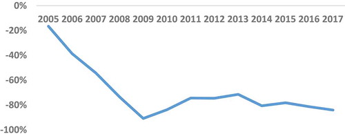
At the first glance, it appears to be alarming as Catao and Milesi-Ferretti (2013) state that four countries (Greece, Ireland, Portugal, and Spain) had NIIP/GDP ratio between (70%) to (90%) when they got into the last global financial crisis. The analysis of the NFL (Figure 2) strongly encourages us to apply the CCA framework to make an immediate assessment of sovereign distress. The CCA framework for Macro-financial risk analysis has analogously been designed on the financial risk assessment model at the firm level. At a firm level, share-price and a market cap of a firm capture the volatility and probability of default. The volatility of local currency liabilities (LCL) is measured by the exchange rate and the quantity of local currency debts. If there is a fixed or managed exchange rate regime (such as Fiji), the major part of volatility will come from the sterilization operations (changes in local currency public debts). Purposefully, the following analysis will bring quantitative risk measures such as distance to distress and probability of default for small sovereign balance sheets such as Fiji.

The present analysis uses the option pricing embedded in the BSM model and the workable framework provided by Gray et al. (2007). This BSM model suggests calculating implied values of assets and their volatilities. Since the subject of this paper is sovereign risk, there is a consolidation of the economic balance sheet of the Government and the Monetary Authority (RBF). The estimates are shown in Table 1. Based on these estimates, two sovereign risk indicators were developed (Table 2).

Table 1. Estimates of key parameters

Year	PV of DB	σDCL$	σAsov$	d1	d2	N(d1)	N(d2)
2014	423.82	9.07	7.64	4.2754	4.1990	0.9999	0.9999
2015	392.31	9.78	8.33	4.6061	4.5228	0.9999	0.9999
2016	417.89	3.92	3.32	2.9062	2.8730	0.9981	0.9979
2017	452.01	7.32	6.27	3.7972	3.7345	0.9999	0.9999

Source: Quarterly RBF Review June 2018 and Author’s estimates

Table 2. Distance and probability to default

Year	Distance to Default (DD)	Implied Probability of Default (IPD)*
2014	2.0230	0.0215
2015	2.0759	0.0189
2016	2.5457	0.0054
2017	2.2642	0.0117

Source: Author’s estimate

The findings indicate a significant decline in the present value of the default barrier in 2015 and d1 and d2 in 2016. The years 2015 and 2016 are significant for Fiji. Fiji was jolted by severe cyclone Winston (category 5) at the beginning of 2015. Total external debts were reduced by 5% and 4 %, respectively, during this period due to excessive inflow of foreign aid for cyclone rehabilitation and the privatization of a few public entities. The international bonds were rolled over successfully at a much lower rate of interest (MOE, 2018, December). However, their probabilities did not change significantly. Based on these variables, there are estimations of DD and the implied PD. The distance to default is in terms of standard deviations and IPD in percentage terms in Table 2.

Table 2 indicates “limited to no sovereign risk” for Fiji. Since this sector has significant foreign currency debt, they also have a huge potential to transmit negative implications to the wider economy—which is abated due to low-risk position. To gain confidence, the distance to default (DD_m) is being compared with the Naïve model (DD_naive).¹⁹ It has helped us to interpret the variations across the methodologies. It has enriched our overall analysis of sovereign distress. Comparative statistics (relative difference in percent) are in Table 3.

Table 3. Comparative analysis of BSM and Naïve

Year	DDm	DDnaive	% diff.	IPDm	IPDnaive	% diff.
2014	2.0230	1.7131	0.31	0.02	0.04	−0.02
2015	2.0759	1.6520	0.42	0.02	0.05	−0.03
2016	2.5457	1.7929	0.75	0.01	0.04	−0.03
2017	2.2643	1.8605	0.40	0.01	0.03	−0.02

Source: Author’s estimate

Both estimates produce similar signals of strong positions and stability, minor differences are due to the use of alternative methodologies. Based on the above analysis, it can be summarized that sovereign risks are low and very much manageable in Fiji. The limiting factor of this analysis is that the contingent liabilities (government guarantees) could not be factored while calculating the distress barrier.

8. Concluding remarks

The CCA framework has the potential for better sovereign risk analysis and applies to even small economies with consistent data. The analysis shows that there is a distance of more than 2 standard deviations from the distress barrier, the probability of sovereign default risk is very low. The calculations have implications for policy, in that, while the Fijian Government is mainly debt financing, it should shop for low-interest debt (below 2%)—IPD compared to the actual average interest rate paid on external debt, indicates that the Government is moving in the right direction. However, this analysis has limitations due to the availability of quality data for doing such analyses.

We are developing the overall framework of macro-financial risk analysis for the South Pacific region. Along with the CCA framework, we have also developed the Foreign Currency Exposure index to gauge the impact of exchange rate volatility on the sovereign balance sheet. The determinants of exchange rate volatility have also been analyzed using co-integration and OLS methods. Currently, we are also linking this research to the wider issue of financial contagion from large economies of the close neighborhood to small economies.

Data derived from public domain resources

1. http://data.imf.org/?sk=4C514D48-B6BA-49ED-8AB9-52B0C1A0179B

2. www.rbf.gov.fj/Statistics/e-GDDS

3. www.rbf.gov.fj/Publications-(1)/Quarterly-Reviews

4. https://www.statsfiji.gov.fj/index.php/statistics/economic-statistics

Data Sources

The sources of data are indicated in A2.

Additional information

Funding

This research did not receive any specific grant from funding agencies in public, commercial, or not-for-profit sectors.

Notes on contributors

Devendra Kumar Jain

Devendra Jain Senior Lecturer in Finance, Westminster International University of Tashkent. Had a distinguished banking career specializing in financial market, banking treasury, currency trading, financial risk management and AML Compliance. Research interests: Macro-Financial Risks, Foreign Currency Exposure and Macro-Financial Risk Indicators.

Rup Singh

Rup Singh Acting Head and Senior Lecturer in Economics, Faculty of Business and Economics (FBE) University of South Pacific (Suva) Fiji. Former Central Banker. Research interests: Economic Growth, Monetary Policy and Applied Econometrics.

Arvind Patel

Arvind Patel Acting Dean and Professor of Accounting and Finance, Faculty of Business and Economics (FBE), University of South Pacific (Suva) Fiji. Distinguished career as an academic and administrator. Research interest: Corporate Governance, Fraud, Ethics and Auditing. Professional memberships to Fiji Institute of Accountants, CPA Australia, American Accounting Association, Accounting Association of Australia and New Zealand and Institute of Internal Auditors.

Notes

1. A contingent claim is defined as a financial contract or derivative whose future value is derived from underlying asset. Financial derivatives such as forwards, futures, and options are examples of contingent claims whose valuations depend on stock-indices, interest rate, exchange rate, commodities, and mortgage-backed securities.

2. Population penalty is used to express the small size of population in island countries. It is referred to as one of the capacity constraints of small economies, Haque, Knight, and Jayasuriya (2012).

3.  Figure A1(Appendix A)-Compares the annual changes in GDP growth of Fiji with average of the Pacific Islands region and the emerging & developing economies average.

4. Impact from 2008 to 2009: Total exports fell from 1471 m to 1230.3 m; Imports from 3601.4 to 2807.9; Visitor arrivals from 585,031 to 542,186: GDP recorded negative growth of −1.4% (RBF Qtr. Review, March 2016).

5. B+ (stable) by S&P (1 May 2015) and B1 (positive) by Moody’s (5 June 2016). https://tradingeconomics.com/fiji/rating.Accessed on 20 August 2017.

6.  Figure A2 (Appendix A) compares General Government Gross Debt (as a percentage of GDP) with the average of the Pacific Islands and the emerging and developing economies.

7. Black & Scholes (1973) model valued contingent claims (options and futures). This option-pricing model was an important tool to analyze and compare asset prices and to measure the risks of financial instruments.

8. The modern theory of CCA has also been successfully used for firm-level analysis.

9.  Gray and Malone (2008) have detailed CCA concepts and descriptions of CCA models.

10. Algebraic solving systems of two equations in two unknowns (variables whose values are not known).

11. The Markov process is a particular type of stochastic process where only the present value of an asset is relevant for predicting future value. It is assumed that the probability distribution of the price at a particular future time is not dependent on past behavior of the price. The Markov stochastic process is identified with a mean zero and variance of 1.

12. A Wiener process is a normal distribution scaled by a factor of √ dt. The drift of the process is zero and the variance rate is 1.00 per unit of time.

13. It is a process where the drift and variance rate of X can be a function of both X itself and time. The changes in X in a very short period of time are normally distributed but not for a longer period of time. For detailed mathematical derivations see (page 217–232 Hull (2003) fifth Edition).

14. A barrier option is dependent on a preset price trigger of an underlying asset. Its exercise or value depends on the barrier events. A perpetual option is an unconventional and non-standard option. It has no expiry date and can be exercised at any point in time.

15. Seniority of liability is not strictly by legal status as in the financial world. Short-term external debt is considered as a senior claim over the assets of a sovereign balance sheet. It is assumed that a sovereign state will prioritize external debt over domestic debt and base money during the period of distress or financial crisis.

16. While valuing implied asset value and expected returns under CCA, it is advised to take risk-adjusted or risk-neutral distribution of asset value by using risk-free interest rate.

17. The detail process of deriving the geometric Brownian motion and Ito’s lemma process is explained in Lu (2008) p 10–24.

18. We intend to develop this analysis further as a future research agenda of the University and regional Governments, under the Pacific Centre for Economic Policy and Modeling, USP.

19. A slight modification is made in the equity return parameter (µ_it-1). We used the simple US 5-year swap rate, rest of the parameters of the Naïve model maintained.

Appendix A

Figure A1. Real GDP Growth (Annual Percentage Change)

Source: IMF: World economic outlook (October 2019)

Figure A2. General government debt (As percentage of GDP)

Source: IMF: World economic outlook (October 2019)

Appendix B Table 4

Table

List of Variables Used
Asov	Implied Value of sovereign assets
σ Asov	Implied Volatility of sovereign assets
σ Asov$	Implied Volatility of sovereign assets in USD
DB	Distress Barrier
DB$	Distress Barrier in USD
DCD	Domestic Currency Debt
DCD$	Domestic Currency Debt in USD
BM	Base Money
BM$	Base Money in USD
FCD	Foreign Currency Debts
DL	Domestic Liabilities
A	Assets
σ A	Volatility of assets
DCL$	Domestic Currency Liabilities in USD
DCL	Domestic Currency Liabilities in local currency
σ DCL$	Volatility of Domestic Currency Liabilities in USD
DCD	Domestic Currency Debt
DCD$	Domestic Currency Debt in USD
σ DCD$	Volatility of Domestic Currency Debt in USD
FR	Forward Rate
σ FR	Volatility of Forward Rate
R,f,t	foreign interest rate up to time
DDsov	Distance to Default or Distress
d1	Conditional probability
d2	Probability adjusted value

Note: σ is volatility, ρ indicates correlation and $ is used to express value in foreign currency

References

- Afik, Z., Arad, O., & Galil, K. (2016). Using Merton model for default prediction: An empirical assessment of selected alternatives. Journal of Empirical Finance, 35(1), 43–17. doi:10.1016/j.jempfin.2015.09.004
- Bharath, S., & Shumway, T. (2004, December 17). Forecasting default with the KMV-merton model. Retrieved from www.citeseerx.ist.psu.edu:http://citeseerx.ist.psu.edu/viewdoc/download?doi=10.1.1.139.1671&rep=rep1&type=pdf
- Black, F., & Scholes, M. (1973). The pricing of options and corporate liabilities. Chicago Journal, 81(3), 637–654.
- Campbell, J., Hilscher, J., & Szilagyi, J. (2008). In search of distress risk. The Journal of Finance, 63(6), 2899–2938. doi:10.1111/j.1540-6261.2008.01416.x
- Catão, L., & Milesi-Ferretti, G. (2013). External liabilities and crises. IMF Working Paper no WP/13/113. pp. 1–30.
- Chava, S., & Jarrow, R. (2004). Bankruptcy prediction with industry effects. Review of Finance, 8, 537–569. doi:10.1093/rof/8.4.537
- Cox, D., & Oakes, D. (1984). Analysis of survival data. New York: Chapman and Hall.
- Crosbie, P., & Bohn, J. (2003). Modeling default risk. New York, NY: Moody's KMV Company.
- Duffie, D., Saita, L., & Wang, K. (2007). Multi-period corporate default prediction with stochastic covariates. Journal of Financial Economics, 83(3), 635–665. doi:10.1016/j.jfineco.2005.10.011
- Galai, D., & Mark, R. (2000). Risk management. New York, NY: McGraw-Hill.
- Gapen, M., Gray, D., Lim, C., & Xiao, Y. (2008). Measuring and analyzing sovereign risk with contingent claims. IMF Staff Working Paper, 55(1), 1–40.
- Gray, D., Merton, R., & Bodie, Z. (2007). Contingent claims approach to measuring and managing sovereign credit risk. Journal of Investment Management, 5(4), 5–28.
- Gray, D., Merton, R., & Bodie, Z. (2009). New framework for measuring and managing macrofinancial risk and financial stability. Central Bank of Chile, Agustinas,wp, 541, 1–35.
- Gray, F., & Malone, W. (2008). Macrofinancial risk analysis. West Sussex UK: John Wiley & Sons Ltd.
- Haque, T., Knight, D., & Jayasuriya, D. (2012). Capacity constraints and public financial management in small pacific Island. The World Bank, Policy Research Working Paper, 6297, 1–36.
- Hull, J. (2003). Options, futures and other derivatives (Fifth ed.). New Jersey: Prentice Hall.
- IMF. (2019, October). World economic outlook. Washignton DC: Author.
- Jayaraman, T., & Choong, C. (2008). Exchange market pressure in a small pacific Island country: A study of Fiji. International Journal of Social Economics, 35(12), 985–1004. doi:10.1108/03068290810911507
- Keller, C., Kunzel, P., & Souto, M. (2007). Measuring sovereign risk in Turkey: An application of the contingent claims approach. IMF, wp 07/233. pp. 1–27.
- Lu, Y. (2008, June 19). Default forecasting in KMV. Retrieved from www.core.ac.uk:https://core.ac.uk/download/pdf/97111.pdf
- Merton, R. C. (1973). Theory of rational option pricing. The Bell Journal of Economics and Management Science, 4(1), 141–183. doi:10.2307/3003143
- MOE. (2018, December). Government of Fiji: Debt Report. Suva: Ministry of Economy, Government of Fiji.
- Narayan, P. (2003). Macroeconomic impact of natural disasters on a small Island economy. Applied Economic Letters, 10(11), 721–723. doi:10.1080/1350485032000133372
- Nazeran, P., & Dwyer, D. (2015). Credit risk modeling of public firms: EDF9. New York, NY: Moody’s Analytics.
- RBF. Quarterly review. (2019). June, Dec 2018, Dec 2016. Suva: Reserve Bank of Fiji.
- Reddy, S. (2008). Impact of the global crisis on Fiji’s economy. BIS Review, (138/2008). pp. 1–4.
- Wainiquolo, I. (2013). Towards a macroeconomic model for Fiji. Reserve Bank of Fiji, Economics Group wp 2013/02. pp. 1–15.