Volatility spillovers between the European and South African foreign exchange markets

Abstract

This article investigates the exchange rate volatility spillover and dynamic conditional correlation between the euro and the South African rand following the Eurozone sovereign debt crisis. It employs two multivariate generalized autoregressive conditional heteroskedasticity (MGARCH) models, namely bivariate BEKK-GARCH (1,1) a nd DCC-GARCH(1,1). Based on two datasets, for the crisis and post-crisis periods, the study identifies significant uni-directional volatility spillovers from the euro to the rand during crisis and post-crisis periods. Further, increased volatility spillovers and time-varying correlations between currencies were evident during the Eurozone crisis. This suggests pure form of financial contagion between the two foreign exchange markets. As such, investors and policy makers in the stock and/or foreign exchange markets in South Africa should monitor euro volatility due to its contagious impacts on the rand and decoupling strategies should be formulated to insulate the rand from contagion. The contributions of the study are twofold. First, it informs the investors in the foreign exchange market on the extent to which shocks in the euro affect the rand. Second, it adds to the literature on pure form of contagion by testing whether there exists an asymmetric correlation between the rand and euro over tranquil periods as opposed to financial upheaval ones.

Keywords:

• BEKK–GARCH
• DCC-GARCH
• volatility spillover
• contagion test

Subjects:

• C32
• F31
• G150

PUBLIC INTEREST STATEMENT

This paper analyses the transmission of shocks between the euro and the South African rand following the currency turbulences in the wake of the Eurozone sovereign debt crisis. The data consist of the daily exchange rates of the rand and euro against the US dollar for 2009–2017. The data were divided into two sub-periods (namely the crisis and post-crisis periods) to contrast the shock transmission intensity between the two sub-periods. During the period of financial upheaval, there existed a significant increase in the strength of shock transmission between the rand and euro. This phenomenon is a pure form of financial contagion, where the transmission of shocks is due to reasons other than economic fundamentals and is rather a result of the irrational behaviours of market participants, such as panic, herd behaviour, and risk aversion.

1. Introduction

Since the South African authorities’ adoption of a free-floating currency regime in 2001, exchange rates are determined by market forces and uncertain returns are a natural outcome (Patnaik, 2013). These uncertain returns—commonly referred to as volatility—may persist over time¹ and give rise to what is usually referred to in the finance literature as volatility clustering or volatility pooling. Volatility may also spread from one market to another, resulting in volatility spillovers (Patnaik, 2013).

This study investigates volatility spillovers to provide insights to investors and policy makers on the volatility dynamics in the South African foreign exchange (FX) market caused by shocks emanating from developed countries in general and from the Eurozone countries specifically. The findings provide information on the formulation and implementation of reliable hedging strategies to protect the rand against the contagious effects of the euro. Furthermore, the study will help policy makers formulate possible decoupling or coupling strategies to insulate the rand from the contagious effects of the euro.

The choice of the South African FX market was motivated by the fact that the South African economy is an emerging market economy (EME). Ozkan and Unsal (2012) stressed that EMEs are more prone to experience volatility spillovers (or financial contagion) due to factors such as their high degree of trade openness and the scale of foreign currency-denominated debt in the domestic economy, commonly known as liability dollarization. The Eurozone FX market was selected as the source (ground zero) market. The choice of the Eurozone market was mainly enthused by the fact that it is South Africa’s largest trading partner and foreign investment source, accounting for 72% of South Africa’s total foreign direct investment stocks (Tralac, 2019).

This study uses multivariate autoregressive conditional heteroskedasticity (MGARCH) models to estimate volatility spillovers and financial contagion. Volatility spillovers have been identified in the academic financial literature “as the cause and/or effect of financial contagion” (Roy & Roy, 2017, p. 1). However, studies such as those of Abou-Zaid (2011) and Diebold and Yilmaz (2009) use the terms volatility spillover and contagion interchangeably. Financial contagion can be defined as “a significant increase in cross-market linkage after a shock to one country or group of countries” (Forbes & Rigobon, 2002, p. 3) and occurs when cross-country correlations increase during crisis periods relative to tranquil periods.

A literature survey identified only one study that investigated the exchange rate volatility spillover in South Africa: Raputsoane (2008) examined volatility spillover between the rand and other currencies in selected developed and emerging markets in Europe, Asia, and Latin America. Using an augmented univariate GARCH model, Raputsoane (2008) found significantly negative exchange rate effects between the rand and European currencies. However, no volatility spillovers were identified between the rand and Asian and Latin American currency markets. However, a standard univariate GARCH model does not consider volatility spillover across markets. Additionally, univariate GARCH models cannot test the significance level of correlation between markets during financial disturbances (Mei, 2016). This study fills this gap by using two multivariate GARCH models. First, the BEKK-GARCH is used to determine the direction of transmission of disturbances between the rand and euro and ensure the positive variance–covariance of a multivariate time series matrix (Carsamer, 2015). Second, the dynamic conditional correlation (DCC)-GARCH model is employed, as it allows correlations to be time-varying in addition to the conditional variances. Hence, this study assesses whether the correlations between the euro and rand are time varying and evolve according to market conditions (e.g., periods of stability versus periods of turmoil).

The rest of this article is structured as follows. Section 2 reviews the literature on volatility spillover in FX markets, Section 3 describes the data and methodology used in the study, and Section 4 discusses the results and findings. Finally, concluding remarks and policy implications are presented in Section 5.

2. Literature review

Studies on the transmission of crises in the context of FX markets include, among others, the pioneering study by Ito et al. (1990), who used meteorological analogies to explain volatility spillovers between the Japanese yen and the US dollar. They posited that the transmission of news can either follow “a heat wave process”, in the sense that “a hot day in New York is likely to be followed by another hot day in New York but not typically by a hot day in Tokyo”, or “a meteor shower process” in which meteors rain down on the earth as it turns; hence, “a meteor shower in New York will almost surely be followed by one in Tokyo” (Ito et al., 1990, p. 4). Using ARCH and GARCH models, they rejected the heat wave hypothesis and found that the yen/dollar FX market is not dextrous (i.e., the equilibrium price does not respond instantaneously and completely to news); instead, it suffers from volatility spillover or volatility clustering because of stochastic policy coordination. Further, Bubák, Kočenda and Žikeš (2011) investigated the dynamics of volatility transmission between Central European currencies and the euro against the US dollar using daily exchange rate volatility based on intraday data. They found strong evidence of spillovers and that volatility spillovers tend to increase in periods characterized by currency market uncertainty. Antonakakis (2012) evaluated spillovers in relation to returns on the euro, British pound, Swiss franc, and Japanese yen against the US dollar before and after the introduction of the euro. He found significant volatility spillovers and co-movements across the four exchange rates and concluded that the volatility declined with the introduction of the euro and suggested that its launch may have brought greater stability in the global financial markets. Moreover, Antonakakis (2012) results indicated that, of the currencies analysed in his paper, the euro is dominant in terms of volatility transmission, as its volatility significantly affects the volatility expectations of the franc, pound, and yen. Xu, Wu, and Wu (2015) studied the dynamic relationship between the renminbi (RMB) and six East Asian currencies, using foreign exchange spot rate data from 2005 to 2013. Using DCC-GARCH and quantile regression models, they found evidence of time-varying correlation and an increasing influence of the RMB in East Asia over the analysed period. They also noted that East Asian currencies behaved differently before the crisis but showed some similarities after it. Xu et al. (2014) also noted that East Asian currencies prefer to “follow” the RMB when it depreciates but are reluctant to do so when it appreciates. They argued this may be related to the different macroeconomic environment in the East Asian region before and after the crisis, China’s rising economic influence, and the internationalization of the RMB. Fratzscher and Mehl (2014) used a three-factor global model of foreign exchange returns to study co-movement between the RMB and East Asian currencies. They found that co-movement is mainly driven by the RMB and co-movements increased markedly after China launched its exchange rate reform in 2005.

Colavecchio and Funke (2008) used switching autoregressive conditional heteroscedasticity time series models to examine volatility dependence between nine Asian markets. Based on the weekly returns on forward exchange rates of the nine countries, they identified two regimes with different volatility levels, each displaying considerable persistence. Pontines and Siregar (2012) used the smooth transition autoregressive model to examine the behaviours of emerging markets in Indonesia, Korea, the Philippines, and Thailand. They found that the central banks of these four economies tend to be more tolerant of the depreciation than the appreciation of their local currencies against the US dollar.

Carsamer (2015) used an unrestricted multivariate BEKK-GARCH model to estimate volatility transmission in selected African countries and found that the FX market on this continent is more susceptible to global market than intra-regional volatility spillovers in for both volatility and mean spillover.

As previously noted, the only study on volatility spillovers in the FX market from a South African perspective is that of Raputsoane (2008), who analysed exchange rate volatility spillovers between the rand and selected currency markets in developed and emerging countries in Europe, Asia, and Latin America. Using a univariate GARCH model, the author found significantly negative exchange rate effects between the rand and European currencies, but no spillover effects between the rand and the Asian and Latin American currency markets.

3. Data and methodology

This section describes the data and econometric models used to investigate the volatility spillovers between the European and South African FX markets, following the Eurozone sovereign debt crisis. The data consist of the daily spot exchange rate of the rand and euro against the US dollar and multivariate GARCH models are used.

3.1. Data

This study used the daily spot exchange rate of the rand and euro against the US dollar from October 2009 to February 2017. All data were sourced from Datastream (Reuters). The study used daily data to obtain a meaningful statistical generalization and a clear picture of the movement of market returns. A potential drawback is the effectiveness of daily data due to trading hour differences; however, as Forbes and Rigobon (2002) stressed, this represents a relative problem and attempts to circumvent the problem by using the average returns failed to find a meaningful difference in their results.

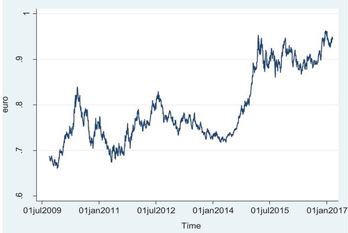
Figures 1 and 2 display the time series plots of the spot exchange rates of the rand and euro against the US dollar, respectively. The time series is non-stationary due to the non-constant mean.

Figure 1. Daily spot exchange rate of the rand against the US dollar from 1 October 2009 to 28 February 2017

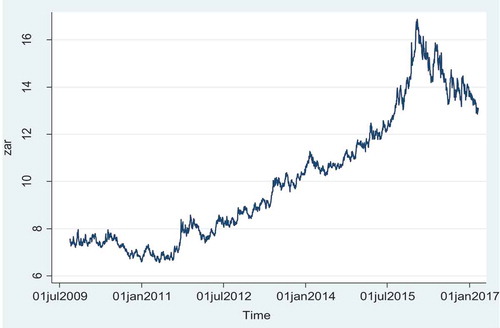
Figure 2. Daily spot exchange rate of the euro against the US dollar from 1 October 2009 to 28 February 2017

To prepare the data for analysis, the spot exchange rates were transformed into logarithmic exchange returns using the following formula:

$R_t=ln\left(P_t\right)-ln\left(P_{t-1}\right)$

where $P_t$ is the spot exchange rate for period t, $P_{t-1}$ is the spot exchange rate for period t-1, and $R_t$ is the logarithmic exchange returns on each currency between times t and t—1. Therefore, $R_t<0$ reflects the appreciation of local currencies against the US dollar. The daily logarithmic exchange returns are displayed in Figures 3 and 4.

Figure 3. Daily changes in logarithmic exchange returns for the rand against the US dollar

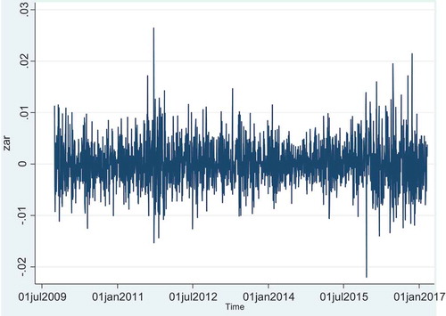
Figure 4. Daily changes in logarithmic exchange returns for the euro against the US dollar

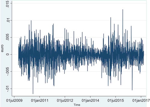
The series display volatility clustering, that is, periods with high volatility are followed by periods of high volatility, and correspondingly, periods with low volatility are followed by periods of low volatility.

3.2. Methodology

As previously mentioned, this study employs two MGARCH models: (1) Engle and Kroner (1995) bivariate BEKK-GARCH, which consists of a conditional covariance matrix and was chosen to determine the direction of transmission of disturbances between the rand and euro and (2) the DCC-GARCH, developed by Engle (2002), to detect the correlation and volatility spillover between the rand and the euro. The models are discussed below.

3.2.1. BEKK-MGARCH

The BEKK-MGARCH model, initially proposed by Engle and Kroner (1995), enables us to reveal the existence of any volatility transmission from one currency to another. The positive definiteness of the conditional covariance matrix is achieved by formulating the model so that this property is implied by the model structure (Yonis, 2011). The following mean equation is estimated for the yield of each currency:

(1) $r_t={\mu }_t+{\epsilon }_t$(1)

${\epsilon }_t\left|{\mathrm{\Omega }}_{t-1}\to \mathrm{N}\right.\left(0,{\mathrm{H}}_t\right)$

where $r_t$ is an 2 × 1 vector of daily exchange rate returns at time t, ${\epsilon }_t$ is a 2 × 1 vector of random errors for each market at time t, ${\mathrm{\Omega }}_{t-1}$ represents the market information that is available at time t-1 with its corresponding 2 × 2 conditional variance-covariance matrix H_t, and $C_t$ is a 2 × 1 vector representing the long-term coefficient drift. The conditional matrix can be written as:

(2) $H_t=C_0^{\prime }C+A_{1,1}^{\prime }{\epsilon }_{t-1}{\epsilon }_{t-1}^{\prime }{A}_{1,1}+G_{1,1}^{\hspace{0.17em}}{H}_{t-1}{G}_{1,1}$(2)

$H_t$ can also take the following form:

(3) $H_t=C_0^{\prime }C+{\left[\begin{array}{cc}{a}_{11}& a_{12}\\ a_{21}& a_{22}\end{array}\right]}^{\prime }\left[\begin{array}{cc}{\epsilon }_{1,t-1}^2& {\epsilon }_{1,t-1}{\epsilon }_{2,t-1}\\ {\epsilon }_{1,t-1}{\epsilon }_{2,t-1}& {\epsilon }_{2,t-1}^2\end{array}\right]\left[\begin{array}{cc}{a}_{11}& a_{12}\\ a_{21}& a_{22}\end{array}\right]+{\left[\begin{array}{cc}{g}_{11}& g_{12}\\ g_{21}& g_{22}\end{array}\right]}^{\prime }{H}_{t-1}\left[\begin{array}{cc}{g}_{11}& g_{12}\\ g_{21}& g_{22}\end{array}\right]$(3)

where

$H_t=\left[\begin{array}{cc}{h}_{11}& h_{12}\\ h_{21}& h_{22}\end{array}\right]$

Further expanded by the matrix multiplication, H_t can also be expressed as:

(4) $h_{11,t}=c_{11}^2+a_{11}^2{\epsilon }_{1,t-1}^2+2a_{11}{a}_{21}{\epsilon }_{1,t-1}{\epsilon }_{2,t-1}+a_{21}^2{\epsilon }_{2,t-1}^2+g_{11}^2{h}_{11,t-1}+2g_{11}{g}_{12}{h}_{12,t-1}+g_{21}^2{h}_{22,t-1}$(4)

(5) $\begin{array}{rl}& h_{12,t}=c_{11}{c}_{12}+a_{11}{a}_{21}{\epsilon }_{1,t-1}^2+\left(a_{21}{a}_{12}+a_{11}{a}_{22}\right){\epsilon }_{1,t-1}{\epsilon }_{2,t-1}+a_{21}{a}_{22}{\epsilon }_{2,t-1}^2+g_{11}{g}_{12}{h}_{11,t-1}\\ & +\left(g_{21}{g}_{12}+g_{11}{g}_{22}\right)h_{12,t-1}+g_{21}{g}_{22}{h}_{22,t-1}\end{array}$(5)

(6) $h_{22,t}=c_{21}^2{c}_{22}^2+a_{12}^2{\epsilon }_{1,t-1}^2+2a_{12}{a}_{22}{\epsilon }_{1,t-1}{\epsilon }_{2,t-1}+a_{22}^2{\epsilon }_{2,t-1}^2+g_{12}^2{h}_{11,t-1}+2g_{12}{g}_{22}{h}_{12,t-1}+g_{22}^2{h}_{22,t-1}$(6)

As Engle and Kroner (1995) posited, since ${\epsilon }_t\left|{\mathrm{\Omega }}_{t-1}\to \mathrm{N}\right.\left(0,{\mathrm{H}}_t\right)$, the above BEKK systems can be estimated efficiently and consistently using the full information maximum likelihood. The log-likelihood function of the joint distribution is the sum of all log-likelihood functions of the conditional distributions, that is, the sum of the logs of the multivariate-normal distribution. Letting $l_t$ be the log-likelihood of observation t, n the number of stock markets, and L the joint log-likelihood, the function takes the following form:

(7) $L\left(\theta \right)={\sum }_{t=1}^p{l}_t\left(\theta \right)\mathrm{a}\mathrm{n}\mathrm{d}{l}_t\left(\theta \right)=-\mathrm{l}\mathrm{o}\mathrm{g}2\pi -\frac{1}{2}log\left|H_t\left(\theta \right)\right|-\frac{1}{2}{\epsilon }_t^{\prime }{H}_t^{-1}\left(\theta \right){\epsilon }_t\left(\theta \right)$(7)

where $L\left(\theta \right)={\sum }_{t=1}^p{l}_t\left(\theta \right)$ denotes the vector of all unknown parameters.

3.2.2. DCC-GARCH

The DCC model was introduced by Engle (2002) to capture dynamic time-varying of conditional covariance. The DCC-GARCH model is a dynamic model with time-varying mean, variance, and covariance of return series $r_t$:

$r_t=u_t+{\epsilon }_t$

${\epsilon }_t\left|{\mathrm{\Omega }}_{t-1}\to \mathrm{N}\right.\left(0,{\mathrm{H}}_t\right)$

From the residuals of the mean equation, the conditional variance of each return is derived as:

(8) $h_{i,t}^2={\alpha }_0+\sum _{j=1}^{p_i}{\alpha }_j{\epsilon }_{i,t-j}^2+\sum _{j=1}^{q_i}{\beta }_j{\sigma }_{i,t-j}^2$(8)

where$\sum _{j=1}^{Pi}{\alpha }_j+\sum _{j=1}^{q_i}{\beta }_j<1$.

Then, the multivariate conditional variance ${\mathrm{H}}_{\mathrm{t}}$ is estimated as follows:

(9) ${\mathrm{H}}_{\mathrm{t}}={\mathrm{D}}_{\mathrm{t}}{\mathrm{R}}_{\mathrm{t}}{\mathrm{D}}_{\mathrm{t}}$(9)

where $H_t$ is the conditional covariance matrix of $r_t$, ${\mathrm{D}}_{\mathrm{t}}$ represents a (k × k) diagonal matrix of time varying standard deviations obtained from the univariate GARCH specifications in Equation (8)(8) $h_{i,t}^2={\alpha }_0+\sum _{j=1}^{p_i}{\alpha }_j{\epsilon }_{i,t-j}^2+\sum _{j=1}^{q_i}{\beta }_j{\sigma }_{i,t-j}^2$(8) , ${\mathrm{R}}_{\mathrm{t}}$ is the (k x k) time varying correlations matrix derived by first standardizing the residuals of mean Equation (1)(1) $r_t={\mu }_t+{\epsilon }_t$(1) of the univariate GARCH model with their conditional standard deviations derived from Equation (8)(8) $h_{i,t}^2={\alpha }_0+\sum _{j=1}^{p_i}{\alpha }_j{\epsilon }_{i,t-j}^2+\sum _{j=1}^{q_i}{\beta }_j{\sigma }_{i,t-j}^2$(8) to obtain ${\eta }_{it}={\epsilon }_{it}/\sqrt{{h_{it}}^2}$.

The standardized residuals are then used to estimate the parameters of conditional correlation as per Equations (10)(10) $R_t={\left(\mathrm{d}\mathrm{i}\mathrm{a}\mathrm{g}\left({\mathrm{Q}}_{\mathrm{t}}\right)\right)}^{-1/2}{Q}_t\left(\mathrm{d}\mathrm{i}\mathrm{a}\mathrm{g}{\left({\mathrm{Q}}_{\mathrm{t}}\right)}^{-1/2}\right)$(10) and (11(11) $Q_t=\left(1-{\theta }_1-{\theta }_2\right)\bar{Q}+{\theta }_1{\eta }_{t-1}\eta {\prime }_{t-1}+{\theta }_2{Q}_{t-1}$(11) ):

(10) $R_t={\left(\mathrm{d}\mathrm{i}\mathrm{a}\mathrm{g}\left({\mathrm{Q}}_{\mathrm{t}}\right)\right)}^{-1/2}{Q}_t\left(\mathrm{d}\mathrm{i}\mathrm{a}\mathrm{g}{\left({\mathrm{Q}}_{\mathrm{t}}\right)}^{-1/2}\right)$(10)

(11) $Q_t=\left(1-{\theta }_1-{\theta }_2\right)\bar{Q}+{\theta }_1{\eta }_{t-1}\eta {\prime }_{t-1}+{\theta }_2{Q}_{t-1}$(11)

where $\bar{Q}$ is the unconditional covariance of the standardized residuals. $Q_t$ does not generally have ones on the diagonal, so it is scaled as in Equation (3)(3) $H_t=C_0^{\prime }C+{\left[\begin{array}{cc}{a}_{11}& a_{12}\\ a_{21}& a_{22}\end{array}\right]}^{\prime }\left[\begin{array}{cc}{\epsilon }_{1,t-1}^2& {\epsilon }_{1,t-1}{\epsilon }_{2,t-1}\\ {\epsilon }_{1,t-1}{\epsilon }_{2,t-1}& {\epsilon }_{2,t-1}^2\end{array}\right]\left[\begin{array}{cc}{a}_{11}& a_{12}\\ a_{21}& a_{22}\end{array}\right]+{\left[\begin{array}{cc}{g}_{11}& g_{12}\\ g_{21}& g_{22}\end{array}\right]}^{\prime }{H}_{t-1}\left[\begin{array}{cc}{g}_{11}& g_{12}\\ g_{21}& g_{22}\end{array}\right]$(3) to derive $R_t$, which is a positive definite matrix. In this model, the conditional correlations are dynamic or time varying. ${\theta }_1$ and ${\theta }_2$ from Equation (11)(11) $Q_t=\left(1-{\theta }_1-{\theta }_2\right)\bar{Q}+{\theta }_1{\eta }_{t-1}\eta {\prime }_{t-1}+{\theta }_2{Q}_{t-1}$(11) are assumed to be positive scalars with ${\theta }_1$ + ${\theta }_2$ < 1.

Finally, the conditional correlation coefficient, ${\rho }_{ij}$, between two foreign exchange rates, i and j, is expressed by the following equation:

(12) ${\rho }_{ij}=\frac{q_{ij,\mathrm{t}}}{\sqrt{q_{ij,\mathrm{t}},q_{jj,\mathrm{t}}}},\mathrm{i},\mathrm{j}=1,2,.......,\mathrm{n},\mathrm{a}\mathrm{n}\mathrm{d}i\ne j$(12)

${\rho }_{ij}=\frac{\left(1-{\theta }_1-{\theta }_2\right){\bar{q}}_{12}+{\theta }_1{\eta }_{1,\mathrm{t}-1}{\eta }_{2,\mathrm{t}-1}+{\theta }_2{q}_{12,t-1}}{\sqrt{\left[\left(1-{\theta }_1-{\theta }_2\right){\bar{q}}_{11}+{\theta }_1{\eta }_{1,t-1}^2+{\theta }_2{q}_{11,\mathrm{t}-1}\right]}\sqrt{\left[\left(1-{\theta }_1-{\theta }_2\right){\bar{q}}_{22}+{\theta }_1{\eta }_{2,t-1}^2+{\theta }_2{q}_{22,\mathrm{t}-1}\right]}}$

The parameters of the DCC model are estimated using the likelihood of this estimator and can be written as:

(13) $L=-\frac{1}{2}\sum _{t=1}^T\left(nlog\left(2\pi \right)+2log\left|D_t\right|+log\left|R_t\right|+\eta {\prime }_t{R}_t^{-1}{\eta }_t\right)$(13)

where $D_t=diag\left\{\sqrt{h_{i,t}}\right\}$ and $R_t$ is the time varying correlation matrix.

One of the stylized facts of financial time series data is that they deviate in two respects from the usual white noise generated under a Gaussian stochastic process. First, the unconditional distribution is severely leptokurtic. In other words, it is more peaked in the centre and displays fat tails, with more unusually large and small observations than would be implied under the Gaussian law. Second, they exhibit volatility clustering, where calm and volatile episodes are observed, so that at least the variance appears predictable (Chinzara & Aziakpono, 2009). Consequently, the Gaussian assumptions in the DCC-GARCH procedure can be violated. To circumvent this problem, this study also uses the t-DCC-GARCH procedure, in which the DCC model is applied under the assumption that market yields follow a multivariate t-distribution, as suggested by Pesaran and Pesaran (2007). To achieve this, Pesaran and Pesaran (2007) introduced the use of devolatilized returns, which are approximately Gaussian, instead of standardized returns.

Devolatilized returns ${\bar{r}}_{it}$ are computed by allowing returns to be normalized by realized volatility rather than by conditional volatilities in GARCH-type models (Barassi et al., 2011).

(14) ${\bar{r}}_{it}=\frac{r_{it}}{{\sigma }_{it}^{{ }^{realised}}}{\tilde{\sigma }}_{it}^2\left(d\right)=\frac{{\sum }_{s=0}^{d-1}{r}_{1,t-s}^2}{d}$(14)

The devolatilized returns, ${\bar{r}}_{it}$, are used in Equation (5)(5) $\begin{array}{rl}& h_{12,t}=c_{11}{c}_{12}+a_{11}{a}_{21}{\epsilon }_{1,t-1}^2+\left(a_{21}{a}_{12}+a_{11}{a}_{22}\right){\epsilon }_{1,t-1}{\epsilon }_{2,t-1}+a_{21}{a}_{22}{\epsilon }_{2,t-1}^2+g_{11}{g}_{12}{h}_{11,t-1}\\ & +\left(g_{21}{g}_{12}+g_{11}{g}_{22}\right)h_{12,t-1}+g_{21}{g}_{22}{h}_{22,t-1}\end{array}$(5) to calculate the conditional correlations.

4. Results and discussion

To test volatility spillovers and time varying correlations between the rand and euro during the Eurozone crisis, this study used two sets of data, namely (1) a crisis period between 1 October 2009 and 29 February 2012 and (2) a post-crisis period between 1 March 2012 and 28 February 2017.²

4.1. Summary statistics

The summary statistics (sample mean, maximum, minimum, median, standard deviation, the kurtosis, and skewness) of the data, namely daily changes in the logarithmic exchange returns of the rand during the crisis and post-crisis periods ($R_{zar,t}^{crisis}$ and $R_{zar,t}^{post-crisis}$), as well as the daily changes in the logarithmic exchange returns of the euro during the crisis and post-crisis periods (the $R_{eu,t}^{crisis}$ and $R_{eu,t}^{post-crisis}$), are listed in Table 1. None of the statistics appear to have a normal distribution, as skewness is non-zero, that is, the market returns of both currencies are either skewed to the right or left and they all appear to be more peaked compared to a standard normal distribution.

Table 1. Summary statistics

	$R_{zar,t}^{crisis}$	$R_{zar,t}^{post-crisis}$	$R_{eu,t}^{crisis}$	$R_{eu,t}^{post-crisis}$
Observations	799	1,085	799	1,085
Mean	0.00015	0.00040	0.00014	0.00020
Minimum	−0.03518	−0.05059	−0.02287	−0.03035
Maximum	0.06081	0.04935	0.02653	0.02400
Standard deviation	0.00996	0.00992	0.00670	0.00546
Skewness	0.39889	0.22870	0.15275	−0.15271
Kurtosis	5.13009	4.89393	3.69046	5.51464

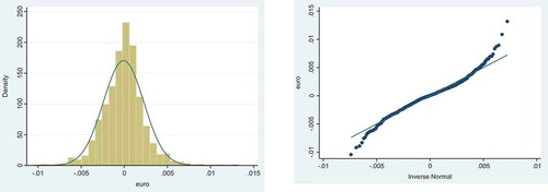
Histograms returns on currencies (overlaid with the curve from a normal distribution) are shown in Figures 5 and 6. The series are leptokurtic, as the centre of the histogram has a high peak and the tails are relatively heavy compared to the normal distribution.

Quantile-quantile (Q–Q) plots for a standard normal Gaussian distribution are also plotted next to each histogram. A theoretical Q–Q plot takes the shape of the line y = x with the data expected to have points lying around the normal prediction line. Deviations of the data points away from this line indicate deviations from normality (Ijumba, 2013). From Figures 5 and 6, the points of the Q–Q plots lie on the normal line, except towards the ends of the plots, indicating the presence of heavy tails.

Figure 5. Density histogram and QQ plot under the Gaussian normal distribution assumption for the yield of the rand versus the US dollar

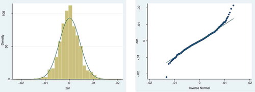
Figure 6. Density histogram and QQ plot under the Gaussian normal distribution assumption for the yield of the euro versus the US dollar

4.2. Estimation of the BEKK-GARCH model

The study first estimates the bivariate BEKK-GARCH model to determine the direction of transmission of disturbances. Additionally, the model effectively captures own and cross volatility spillovers between the two currency markets. Tables 2 and 3 present the estimated coefficients from the variance-covariance matrix of the bivariate BEKK-GARCH model used to analyse the volatility relationship between the rand and euro. The estimates are presented for both the crisis and post-crisis periods.

Table 2. Summary of the BEKK-GARCH model parameter estimates for the rand and euro during the crisis period

	Estimate	Std. error
C11	−0.00612***	0.000377
C12	−0.02073***	0.000579
C22	0.005191***	0.000737
A11	−0.06765	0.07247
A12	0.548501***	0.09458
A21	−0.09757	0.043888
A22	−0.50218***	0.056842
G11	−0.08569	0.193077
G12	−0.05205	0.087893
G21	0.280459***	0.106543
G22	−0.2422	0.082126

***, **, and * significant at 1%, 5%, and 10%, respectively.

Table 3. Summary of the BEKK-GARCH model parameter estimates for the rand and euro during the post-crisis period

	Estimate	Std. error
C11	0.005054***	0.001065
C12	0.004255	0.00561
C22	0.006536***	0.000842
A11	0.302989***	0.047744
A12	−0.10482*	0.030514
A21	−0.01929	0.032267
A22	0.396738***	0.052174
G11	−0.17188	0.618079
G12	0.747106	1.643285
G21	−0.04441	0.389596
G22	0.169976	0.612032

***, **, and * significant at 1%, 5%, and 10%, respectively.

Considering the parameter estimates, the diagonal values in matrix A indicate own innovation (ARCH effects) spillover and the diagonal values in matrix G represent persistence in own conditional volatility (GARCH effects).

From Table 2, A₂₂ is statistically significant. This indicates the presence of the rand’s own volatility spillover effects during the crisis period. In other words, the current volatility of the rand is highly dependent on its volatility in the previous period. Conversely, Table 2 indicates that parameter A₁₁ for the euro is not statistically significant, meaning that its own volatility spillover was negligible during the crisis period. The analysis could not identify the presence of own conditional variance in both currencies, as both diagonal matrices G₁₁ and G₂₂ were statistically insignificant for the crisis period.

The crisis period off-diagonal matrices A and G in Table 2 capture cross-market effects, such as shock and volatility spillover. There is a uni-directional linkage in the transmission of shocks from the euro to the rand, as the parameter A₁₂ is the only statistically significant off-diagonal parameter.

The results of the parameter estimates in Table 3 for the post-crisis period yield results similar to the crisis period. However, it is worth noting that parameter A₁₂ for the post-crisis period is negative, indicating the presence of anti-correlation.

The above results indicate that volatility transmission in the South African FX market follows the meteor shower hypothesis. These results are also in line with Carsamer (2015), who found strong evidence of persistent volatility spillovers between South Africa and United Kingdom’s (UK) FX markets. However, for the UK, transmission was bidirectional.

4.3. Estimation of the DCC-GARCH model

Summary estimates of the DCC-GARCH model parameters are displayed in Table 4. The univariate GARCH(1,1) parameter estimates for each of the currency yields, represented by diagonal elements D_t, are as defined in Equation (9)(9) ${\mathrm{H}}_{\mathrm{t}}={\mathrm{D}}_{\mathrm{t}}{\mathrm{R}}_{\mathrm{t}}{\mathrm{D}}_{\mathrm{t}}$(9) , whereas ${\theta }_1$ and ${\theta }_2$ represent the DCC conditional correlation parameters.

Table 4. Summary of parameter estimates for the DCC model during the crisis period

	Parameter	Estimate
$R_{zar,t}^{crisis}$	${\alpha }_0$	8.93e-06
	$\sum _{j=1}^{p_i}{\alpha }_j$	0.10665***
	$\sum _{j=1}^{q_i}{\beta }_j$	0.80302 ***
$R_{eu,t}^{crisis}$	${\alpha }_0$	0.00002*
	$\sum _{j=1}^{p_i}{\alpha }_j$	0.12264 ***
	$\sum _{j=1}^{q_i}{\beta }_j$	0.45454*
	${\theta }_1$	0.03607**
	${\theta }_2$	0.89713***
${\rho }_{ij}$[corr (zar, euro)]		0.58724
Maximized log likelihood		5,599.10100

*****, and * significant at 1%, 5%, and 10%, respectively.

The parameter estimates for the crisis period appear significantly different from zero. Moreover, 1the sum of the estimates, $\left(\sum _{j=1}^{p_i}{\alpha }_j+\sum _{j=1}^{q_i}{\beta }_j\right)$, is less than unity for both returns (0.98957 for the rand and 0.57718 for the euro). For the euro, sum $\sum _{j=1}^{p_i}{\alpha }_j+\sum _{j=1}^{q_i}{\beta }_j$ is 0.57718, which indicates a relatively lower persistence of volatility during the crisis period.

However, the DCC correlation parameters for the crisis period differ from zero, implying that the correlation between the two currencies is dynamic. Additionally, the correlation parameter estimates show adherence to the restriction imposed on them, that is, ${\theta }_1$+${\theta }_2$ = 0.93320 <1.

As indicated in Table 1 the Gaussian assumption in the DCC-GARCH model on the return of the two currencies is violated. To capture the fat-tailed nature of returns, the DCC model was combined with t multivariate distributions. The results for the crisis period using t-DCC are displayed in Table 5.

Table 5. Summary of parameter estimates for the t-DCC model during the crisis period

	Parameter	Estimate
$R_{zar,t}^{crisis}$	${\alpha }_0$	6.45e-06
	$\sum _{j=1}^{p_i}{\alpha }_j$	0.09958**
	$\sum _{j=1}^{q_i}{\beta }_j$	0.83632***
$R_{eu,t}^{crisis}$	${\alpha }_0$	0.00002
	$\sum _{j=1}^{p_i}{\alpha }_j$	0.10161***
	$\sum _{j=1}^{q_i}{\beta }_j$	0.54928
	${\theta }_1$	0.02895
	${\theta }_2$	0.92106***
${\rho }_{ij}$[corr (zar, euro)]		0.59946***
Maximized log likelihood		5,627.95900

***, **, and * significant at 1%, 5%, and 10%, respectively.

The results of the t-DCC-GARCH model in Table 5 show similar results to the normal DCC-GARCH; however, parameter estimates $\sum _{j=1}^{q_i}{\beta }_j$ and ${\theta }_1$ are not statistically significant. This means conditional volatility is negligible for the euro. These results confirm the findings obtained using the BEKK-GARCH model displayed in Table 2. Given that the maximum likelihood values for t-DCC GARCH are greater than those for the normal DCC-GARCH (5627.959 > 5599.101), we conclude that t-DCC is the most appropriate model to capture the fat-tailed nature of the returns.

Parameter estimates for the post-crisis period were also computed and are displayed in Table 6.

Table 6. Summary of parameter estimates for the DCC model during the post-crisis period

	Parameter	Estimate
$R_{zar,t}^{crisis}$	${\alpha }_0$	1.51e-06*
	$\sum _{j=1}^{p_i}{\alpha }_j$	0.04911 ***
	$\sum _{j=1}^{q_i}{\beta }_j$	0.93644 ***
$R_{eu,t}^{crisis}$	${\alpha }_0$	5.49e-07***
	$\sum _{j=1}^{p_i}{\alpha }_j$	0.06012 ***
	$\sum _{j=1}^{q_i}{\beta }_j$	0.92202***
	${\theta }_1$	0. 02503**
	${\theta }_2$	0.94301***
${\rho }_{ij}$[corr (zar, euro]		0.34113 ***
Maximized log likelihood		7,748.14600

***, **, and * significant at 1%, 5%, and 10%, respectively.

The parameter estimates for the post-crisis period also appear significantly different from zero. The significance of the univariate GARCH parameters $\sum _{j=1}^{p_i}{\alpha }_j$ and $\sum _{j=1}^{q_i}{\beta }_j$ and sum $\left(\sum _{j=1}^{p_i}{\alpha }_j+\sum _{j=1}^{q_i}{\beta }_j\right)$ being close to unity implies that conditional volatility for both the euro and rand is highly persistent. Moreover, the sum of the estimates, $\left(\sum _{j=1}^{p_i}{\alpha }_j+\sum _{j=1}^{q_i}{\beta }_j\right)$, is less than unity for both returns (i.e., 0.84956 for the rand and 0.72571 for the euro).

However, the DCC-GARCH correlation parameters for the post-crisis period are also different from zero, implying the correlation between the two currencies is dynamic. Additionally, the correlation parameter estimates show adherence to the restriction imposed on them, that is, ${\theta }_1$ + ${\theta }_2$ = 0.96120 < 1, suggesting that estimated correlation matrix Dt is positively defined.

We also use the t-DCC-GARCH model to capture the fat-tailed nature of returns during the post-crisis period. The results for the post-crisis period using the t distribution are displayed in Table 7.

Table 7. Summary of parameter estimates for the t-DCC model during the post-crisis period

	Parameter	Estimate
$R_{zar,t}^{crisis}$	${\alpha }_0$	1.40e-06
	$\sum _{j=1}^{p_i}{\alpha }_j$	0.05660***
	$\sum _{j=1}^{q_i}{\beta }_j$	0.93297***
$R_{eu,t}^{crisis}$	${\alpha }_0$	3.90e-07**
	$\sum _{j=1}^{p_i}{\alpha }_j$	0.06161***
	$\sum _{j=1}^{q_i}{\beta }_j$	0.92500 ***
	${\theta }_1$	0.02509***
	${\theta }_2$	0.95245***
corr (zar, euro)		0.36389
Maximized log likelihood		7,808.54500

***, **, and * significant at 1%, 5%, and 10%, respectively.

The results of the t-DCC-GARCH model in Table 7 are in line with those of the normal DCC-GARCH. The maximum likelihood values for t-DCC-GARCH are greater than those for the normal DCC-GARCH (7808.54500 > 7748.14600); hence, the t-DCC model is the most appropriate model to capture the fat-tailed nature of the returns.

A graphical representation of conditional correlation between the rand and euro over time is presented in Figures 7 and 8 for the crisis and post-crisis periods, respectively.

Figure 7. Conditional correlation between the rand and euro during the crisis period

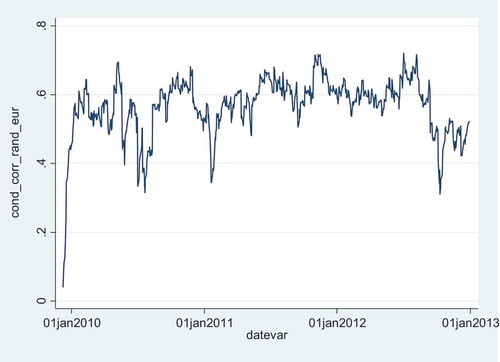
Figure 8. Conditional correlation between the rand and euro during the post-crisis period

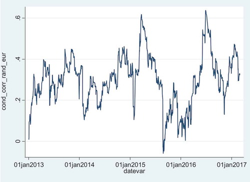
During the crisis period, the conditional correlation was relatively high compared to the post-crisis period. Throughout the crisis period, the conditional correlation remained positively high. Conversely, during the post-crisis period, the correlation decreased significantly and even reached negative values towards the end of 2015. Interestingly, the period of negative correlation coincides with a period of volatility in the rand caused by what is commonly known as Nenegate, that is, when the South African president controversially sacked his then finance minister Mr. Nhlanhla Nene, resulting in a sharp weakening of the rand.

The fact that the conditional correlation between the rand and euro is significantly higher during tranquil periods compared to crisis periods suggests the presence of financial contagion between the European and South African FX markets.

5. Conclusions and policy implications

This study investigated the behaviour of the rand vis-à-vis the euro before and after the recent Eurozone sovereign debt crisis to determine whether there existed volatility spillovers between the two currencies during the crisis. Multivariate GARCH models were employed using two sets of data—for the crisis and post-crisis periods. We found evidence of volatility spillovers and time-varying correlation between the euro and rand in both periods.

We also found evidence that the volatility spillover from the euro to the rand is unidirectional and volatility is more prevalent during periods of turmoil than during stable periods. Hence, financial contagion took place between the European and South African FX markets.

Since the volatility spillovers between the euro and rand are unidirectional, the policy implications are as follows: (i) policy makers, traders, investors, and regulatory authorities should focus on monitoring the volatility of the euro as the efforts by the South African authorities to stabilize volatility spillovers from the euro to rand are futile because volatility emanates from the Eurozone countries; (ii) the regulatory authorities should formulate international economic policies and macro-prudential regulations that enable investors to significantly reduce the risk exposure of the rand to the euro; (iii) international trading firms in South Africa should formulate and implement reliable hedging strategies against the contagious effects of the euro to serve as shock absorber of volatilities emanating from EU markets; and (iv) South African authorities should also strive to increase the attractiveness of the country’s goods and services to other markets besides the EU, which will help decrease the co-movement of economic cycles between the two markets. Finally, it is imperative that the regulatory, supervisory, and monetary authorities work together to formulate a comprehensive regulatory framework that allows investors and traders to benefit from increased currency stability.

Additional information

Funding

This work was supported by the South African Reserve Bank, through the financial stability grant. The work was also presented at Financial stabilitly research conference on 26 & 27 October 2017.

Notes on contributors

Olivier Niyitegeka

Olivier Niyitegeka is a lecturer with the Regent Business School and a PhD student at the University of Zululand. His research interests include international economics, behavioural finance, financial risk management, time series analysis of macroeconomic variables, and development economics.

Devi Datt Tewari

Devi Datt Tewari is a professor with the Department of Economics, Faculty of Commerce, Administration and Law, University of Zululand. Professor Tewari holds a PhD from the University of Saskatchewan, Canada. He has published eight books and more than 100 articles in peer reviewed journals.

Notes

1. That is, periods of high volatility are followed by periods of high volatility and periods of low volatility are followed by periods of low volatility.

2. While other studies use a crisis and a pre-crisis period, the authors are of the opinion that the period prior to the Eurozone crisis was also characterized by financial turmoil and is thus not a good representation of a tranquil period.

References

- Abou-Zaid, A. S. (2011). Volatility spillover effects in emerging MENA stock markets. Review of Applied Economics, 7(1076–2016–87178), 107–17. https://ageconsearch.umn.edu/record/143429/
- Antonakakis, N. (2012). Exchange return co-movements and volatility spillovers before and after the introduction of euro. Journal of International Financial Markets, Institutions and Money, 22(5), 1091–1109. https://doi.org/10.1016/j.intfin.2012.05.009
- Barassi, M., Dickinson, D., & Le, T. (2011, August 4–6). TDCC GARCH modeling of volatilities and correlations of emerging stock markets. In Singapore Economics Review Conference, Mandarin Orchard Singapore.
- Bubák, V., Kočenda, E., & Žikeš, F. (2011). Volatility transmission in emerging European foreign exchange markets. Journal of Banking & Finance, 35(11), 2829–2841. https://doi.org/10.1016/j.jbankfin.2011.03.012
- Carsamer, E. (2015). Exchange rate co-movement and volatility spill over in Africa. National Institute of Development Administration. http://libdcms.nida.ac.th/thesis6/2014/ba188419.pdf.
- Chinzara, Z., & Aziakpono, M. J. (2009). Dynamic returns linkages and volatility transmission between South African and world major stock markets. Studies in Economics and Econometrics, 33(3), 69–94. https://journals.co.za/content/bersee/33/3/EJC21489
- Colavecchio, R., & Funke, M. (2008). Volatility transmissions between renminbi and Asia- Pacific on-shore and off-shore US dollar futures. China Economic Review, 19(4), 635–648. https://doi.org/10.1016/j.chieco.2008.05.003
- Diebold, F. X., & Yilmaz, K. (2009). Measuring financial asset return and volatility spillovers, with application to global equity markets. The Economic Journal, 119(534), 158–171. https://doi.org/10.1111/j.1468-0297.2008.02208.x
- Engle, R. (2002). Dynamic conditional correlation: A simple class of multivariate generalized autoregressive conditional heteroskedasticity models. Journal of Business & Economic Statistics, 20(3), 339–350. https://doi.org/10.1198/073500102288618487
- Engle, R. F., & Kroner, K. F. (1995). Multivariate simultaneous generalized ARCH. Econometric Theory, 11(1), 122–150. https://doi.org/10.1017/S0266466600009063
- Forbes, K. J., & Rigobon, R. (2002). No contagion, only interdependence: Measuring stock market comovements. The Journal of Finance, 57(5), 2223–2261. https://doi.org/10.1111/0022-1082.00494
- Fratzscher, M., & Mehl, A. (2014). China’s dominance hypothesis and the emergence of a tri‐ polar global currency system. The Economic Journal, 124(581), 1343–1370. https://doi.org/10.1111/ecoj.2014.124.issue-581
- Ijumba, C. (2013). Multivariate analysis of the BRICS financial markets [Unpublished master’s thesis]. University of KwaZulu-Natal.
- Ito, T., Engle, R. F., & Lin, W. L. (1990). Where does the meteor shower come from? The role of stochastic policy coordination (No. w3504). National Bureau of Economic Research.
- Mei, G. (2016, December 19). University of Colorado Boulder. https://scholar.colorado.edu/honr_theses/1195/
- Ozkan, M. F. G., & Unsal, D. F. (2012). Global financial crisis financial contagion, and emerging markets (No. 12-293). International Monetary Fund.
- Patnaik, A. (2013). A study of volatility spillover across select foreign exchange rates in India using dynamic conditional correlations. Journal of Quantitative Economics, 11(1/2) 28–47.https://www.econbiz.de/Record/a-study-of-volatility-spillover-across-select-foreign-exchange-rates-in-india-using-dynamic-conditional-correlations-patnaik-anuradha/10010338354
- Pesaran, B., & Pesaran, M. H. (2007). Modelling Volatilities and Conditional Correlations in Futures Markets with a Multivariate t Distribution (No. 2906). Institute of Labor Economics (IZA).
- Pontines, V., & Siregar, R. Y. (2012). Exchange rate asymmetry and flexible exchange rates under inflation targeting regimes: Evidence from four East and Southeast Asian countries. Review of International Economics, 20(5), 893–908. https://doi.org/10.1111/roie.12002
- Raputsoane, L. (2008). Exchange rate volatility spillovers and the South African currency.In TIPS Annual Conference (eds), Annual Forum 2008: South Africa’s Economic Miracle – Has the Emperor Lost his Clothes? South Africa: TIPS, 1-16. http://www.tips.org.za/files/Leroi_Exchange_rate_volatility_spillovers-24_Oct_2008.pdf
- Roy, R. P., & Roy, S. S. (2017). Financial contagion and volatility spillover: An exploration into Indian commodity derivative market. Economic Modelling, 67(2017), 368–380. https://doi.org/10.1016/j.econmod.2017.02.019
- Tralac. (2019). South Africa: A 2018 trade and investment profile. Trade Law Centre (Tralac). https://www.tralac.org/publications/article/13932-south-africa-a-2018-trade-and- investment-profile.html
- Xu, X., Wu, S., & Wu, Y. (2015). The relationship between renminbi’s exchange rate and east asia currencies before and after the “financial crisis”. China Finance Review International.
- Yonis, M. (2011). Stock market co-movement and volatility spillover between USA and South Africa [Unpublished master’s thesis]. Umeå,Universitet.