The behaviour of the real effective exchange rate of South Africa: Is there a misalignment?

Abstract

This paper examines the extent of misalignment of the real effective exchange rate (REER) of South African rand. With South Africa being an open emerging market economy closely linked with global markets, the country’s economy is susceptible to external shocks and changes in global trade patterns. Based on the behavioural equilibrium exchange rate framework of Clark and MacDonald (1998) the study uses a cointegration technique, which caters for endogeneity to estimate the equilibrium value of the REER of the rand. Next, the study uses a Markov regime-switching (MSM) method to determine whether the exchange rate’s departure from the equilibrium level is meaningful enough to be considered as either over- or undervalued. The results show that long-run equilibrium relationship between the rand’s REER and economic variables inclusive of terms of trade, external openness, capital flows and government expenditure. The MSM correctly captures exchange rate misalignment as distinct episodes of exchange rate overvaluation and undervaluation. Most of the exchange rate undervaluation episodes identified in the study have been in response to either idiosyncratic shocks emanating from internal economic/political challenges or systemic global factors transmitted through either the nominal exchange rate or capital flows and not policy-induced behaviour.

Keywords:

• exchange rate
• misalignment
• ARDL
• Markov regime-switching
• economic growth

Subjects:

• F31
• F41

PUBLIC INTEREST STATEMENT

This paper analyses the behaviour of the exchange rate of the South African rand to determine whether it is misaligned. The study uses quarterly data from 1990 to 2018. This study finds evidence that a long-run equilibrium relationship exists between the real effective exchange rate of the rand and the terms of trade, external openness, capital flows, investment and government expenditure. The results show that the exchange rate deviates from its equilibrium level over time and that the exchange rate has been, on average, more overvalued than undervalued over the period covered in study. The undervaluations episodes have tended to be abrupt and at times extreme with a quick correction and sharp movement to overvaluation. Most of the exchange rate undervaluation episodes identified have been in response to either idiosyncratic shocks emanating from internal economic/political challenges or systemic global factors transmitted through either the nominal exchange rate or capital flows and not policy-induced behaviour.

1. Introduction

The exchange rate remains arguably one of the most closely watched economic indicators by policymakers, financial market participants and industries involved in international trade. Since it reflects a country’s competitiveness in international markets, the exchange rate has a major influence on economic activity mainly through the external sector. Exchange rate misalignment, when the exchange rate deviates from its long-run equilibrium level resulting in either an over- or undervalued currency, has generated wide interest in recent years due to increased levels of external openness that support global trade and capital flows. There is evidence in the literature to suggest that keeping the exchange rate close to its equilibrium level is a necessary pre-condition for growth, with countries that avoid currency overvaluation linked to export-led economic growth and export diversification (Elbadawi et al., 2012).

Debate about the equilibrium level of the South African rand and the factors driving the currency are ongoing, with a concomitant lack of consensus on the most appropriate level of the exchange rate in line with the country’s economic fundamentals. Within this context, the aim of this paper is to determine the extent to which the rand’s real effective exchange rate (REER) is misaligned with its equilibrium level. This is achieved via the following manner: (i) use co-integration techniques in the Behavioural Equilibrium Exchange Rate (BEER) framework of Clark and MacDonald (1998) to estimate the equilibrium value of the rand consistent with economic fundamentals; and (ii) interpret the deviation of the observed exchange rate from this equilibrium level as REER misalignment. In a similar fashion to Terra and Valladares (2010), a Markov regime-switching (MSM) is then applied to quantify whether the exchange rate’s departure from the equilibrium level is meaningful enough to be considered as either over- or undervalued.

The paper is structured as follows: Section 2 provides a historical background of the rand’s movements with reference to developments in the South Africa’s economy. Section 3 presents a review of relevant previous studies on exchange rate modelling in South Africa. The empirical method applied is presented in Section 4, with the results presented in Section 5. The conclusion and policy implications are provided in Section 6.

2. Exchange rate performance in South Africa

The evolution of the exchange rate (both nominal and real) is represented in Figure 1, which indicates that the nominal effective exchange rate (NEER) has depreciated most of the time since 1970. The REER, on the other hand, has undergone periods of cyclical movement with appreciation periods followed by subsequent weakening in the currency, with movements in the exchange rate also indicating the presence of volatility. Between 1970 and 2018, about five REER major directional currency movement episodes can be identified: two appreciation and two depreciation periods.

From the early 1970 s up until the pre-1994 democratic elections, political tensions in South Africa, economic sanctions and capital controls had a major influence on the country’s exchange rate movements. This period was marred by a consistent depreciation in the nominal exchange rate, capital outflows, low GDP growth and a positive balance on the current account. Although the 1985 debt crisis (where foreign banks recalled their loans to South Africa with no new credit extended) caused a sharp decline in the exchange rate, the REER appreciated modestly between 1986 and 1993 with the index rising from around 81 in 1986 to 111.04 at the end of 1992, mainly on the back of a decline in South Africa’s inflation rate. The period between 1993 and 2001 saw the REER index decline from above 110 to reach 71 at the end of 2001, with the currency depreciating steeply between 1998 and 2001. This took place against the backdrop of improved macroeconomic performance and a re-integration of the country into the global economy following the successful transition to democracy in 1994. A number of factors may have been responsible for this, such as possible contagion effect of the 1997–1998 Asian financial crisis, low global commodity prices and speculative attacks on the currency.

Figure 1. Rand REER and NEER historical performance: 1970–2018.

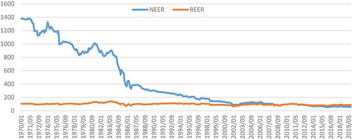
The currency recovered sharply from the end of 2001, resulting in an appreciation episode from 2002 until 2006 where the REER strengthened by around 34%. This episode was driven by an appreciation in the NEER and declines in the inflation rate. The extent and speed of the recovery in the rand suggest that the currency might have been highly undervalued in 2001, thus necessitating a correction. As noted by Saayman (2007), the strengthening currency in 2002 raised debate about the appropriate level of the exchange rate and competitiveness of South African exports with mining companies, the manufacturing sector and labour movements being the most vocal about the negative economic impact of the stronger currency.

Another episode occurred following the global financial crisis in 2007 and the subsequent collapse in global trade flows, the decline in economic performance and the increase in global financial market volatility (especially risk perception towards emerging markets such as South Africa). The REER declined from 90.78 at the beginning of 2007 to 77.55 in 2008Q4 before regaining about 30% to recover and reach a level of 106.76 in 2010Q2. The REER depreciated gradually from this 2010 level to end 2014 at 81.20. Between 2008Q3 to 2011Q4 the values of REER and NEER coincided, but from 2012Q1, the value of the REER continues to be higher than the NEER. Such developments, especially the extent of the weakness in the nominal exchange rate, again raised apprehension about whether such movements reflect South Africa’s economic fundamentals and whether the currency was correctly priced, or whether this signified a misalignment in the exchange rate.

3. Literature review

On a broad level, estimation of equilibrium exchange rates has taken theoretical approaches based on either the Fundamental Equilibrium Exchange Rate (FEER) methodology (macroeconomic balance or external sustainability) or the BEER approach (equilibrium exchange rate) with several variations of both approaches identifiable in the literature (Aflouk, Jeong, Mazier & Saadaoui, 2010). Lòpez-Villavicencio et al. (2012, p. 60) state that despite the conceptual differences, FEER and BEER methodologies rather complement one another instead of being substitutes. The BEER approach is the preferred approach for the study for its practical approach to equilibrium exchange rate estimation and ease of application to developing countries (Gan et al., 2013). A major shortcoming of the fundamental equilibrium exchange rate approach is that the equilibrium level of the exchange rate is highly influenced by the normative assumptions around the internal (full employment and low employment condition) and external balance (sustainable current account) positions (Ajevskis et al., 2012). The BEER method on the other hand is highly statistical and free of normative judgements.

Empirical literature on exchange rate modelling and REER misalignment across countries is abundant. Given the wide-ranging nature literature, the review presented is not exhaustive and focuses on studies specific to South Africa. Aron et al. (1997) are credited with pioneering modelling of the rand’s long-run equilibrium real exchange rate. Using quarterly data from 1970 to 1995, they employ cointegration and error correction methodology to model the long- and short-run determinants of the real exchange rate within the macroeconomic balance approach. Their study concludes that the exchange rate is a function of variables such as trade policy, terms of trade, capital flows, technology, official reserves and government expenditure. Aron et al. (1997) find that the real exchange rate fluctuates over time to reflect changes in several economic fundamentals and shocks to the economic system.

MacDonald and Ricci (2004) use the BEER method within a vector error correction model (VECM) framework to estimate a long-run cointegrating relationship between the REER and economic variables over the period from 1970 to 2002. They find that long-run real exchange rate movements in South Africa could be explained by commodity price movements, productivity,¹ real interest rate differentials against trading partners, the fiscal balance, net foreign assets position and trade openness. Several manifestations of exchange rate misalignment were identified in the study, confirming that the rand was undervalued by more than 25% in early 2002 following the sharp depreciation in the nominal exchange rate in 2001. MacDonald and Ricci (2004) state that deviations from the equilibrium exchange rate would normally be eliminated within a short period of time if there are no other shocks to the system (8% speed of adjustment in the cointegrating equation).

Du Plessis (2005) raises the important issue of endogeneity in econometric modelling and questions the validity of MacDonald and Ricci (2004) results since the exchange rate was weakly exogenous in their preferred model. Besides the existence of an equilibrium relationship between the real exchange rate and the economic fundamentals, Du Plessis (2005) states that the other condition necessary for an equilibrium exchange rate model is that the exchange rate should be endogenous in the model such that disequilibria must have a feedback effect on the real exchange rate. With MacDonald and Ricci’s model violating the condition of endogeneity, Du Plessis (2005) concludes that their model does not qualify as an equilibrium exchange rate model. In response to Du Plessis (2005), MacDonald and Ricci (2005) extend their data by six quarters to address the issue and argue that limited degrees of freedom explained the weak exogeneity. The authors also contend that the absence of weak endogeneity does not significantly affect their equilibrium model.

Saayman (2007) estimates the BEER using different measures of the real exchange rate (price inflation, cost inflation and labour cost adjusted real exchange rates). Also applying a VECM, the objective was to ascertain how the different real exchange rate measures influence the equilibrium long-run exchange rate and the extent of misalignment. Using relative GDP rates (measured as the log of relative GDP per capita of South Africa versus the United States (US)), real interest rate differentials, terms of trade, net foreign assets, gold price, trade openness, the fiscal balance, government expenditure, gross reserves and a commodity index as explanatory variables, the author finds that the equilibrium exchange rate follows a similar path irrespective of the specification of the real exchange rate. In a more recent paper, Saayman (2010) uses BEER methodology and applies Fully Modified Ordinary Least Squares (FMOLS) and Dynamic OLS (DOLS) methods in a panel approach to identify the determinants of the long-run equilibrium exchange rate of the rand against the US dollar, British pound, Japanese yen and the euro together with episodes of exchange rate misalignment. The study finds episodes of both over- and undervaluation of South Africa’s long-run equilibrium exchange rate, although the currency would revert to equilibrium within a short period. Both studies by Saayman (2007, 2010) focus on bilateral real exchange rates as opposed to the REER which is more reflective of the country’s external competitiveness.

A study by De Jager (2012) follows the BEER approach and applies a VECM to examine the various economic indicators that influence the REER; and further model the equilibrium real exchange rate and the extent of exchange rate misalignment using data from 1982 to 2011. De Jager (2012) separates the explanatory variables into five broad areas: the financial sector, commodity prices and terms of trade, the fiscal balance sector, and the real and international sectors, and concludes that trends in economic fundamentals play an essential role in determining the equilibrium exchange rate. The study confirms that the REER can deviate from its equilibrium level and affirms the findings by MacDonald and Ricci (2004) that the rand was undervalued by about 20% in early 2001. De Jager (2012) cautions that the equilibrium real exchange rate level is a function of the set of fundamentals specified in the model, and accordingly notes that results would differ should the model be specified differently. One shortcoming of the study is that it makes no reference to endogeneity in the model as specified by Du Plessis (2005).

The limited studies that consider REER equilibrium levels and exchange rate misalignment in South Africa apply a similar methodology (linear cointegration methods) with all of them (except for De Jager, 2012) using data predating the global financial crisis. The exchange rate, in a similar fashion to other financial variables, is subject to abrupt changes in behaviour which linear modelling methods sometimes cannot capture appropriately. Nonlinear models, on the other hand, are better suited to capture sharp and discrete changes in the economic mechanism that generates the data being studied, hence the increasing popularity of Markov switching frameworks in modelling financial time series. Since exchange rate misalignment could be considered to exhibit two distinctly separate sets of behaviour, a regime switching methodology—which captures these characteristics—might be more appropriate to model such behaviour.

This study adds to the literature in the following aspects: firstly, recent data is applied to estimate the equilibrium REER and exchange rate misalignment; secondly, the subject of exogeneity in the equilibrium exchange rate model is addressed to ensure a proper specification is obtained. Finally, the study uses a nonlinear regime switching methodology to model the misalignment behaviour such that the rand’s misalignment dynamics are seen as originating from one of the two distinct regimes, namely over- or undervaluation episodes. With the exception of Terra and Valladares (2010) who include South Africa in a panel specification, the authors have no knowledge of a study that has used a similar approach.

4. Methodology

4.1. BEER framework and exchange rate misalignment

The BEER approach focuses on modelling the behavioural link between real exchange rates and the appropriate economic variables using a reduced-form equation. This method is aimed at identifying statistically significant long-term drivers of the REER and subsequently modelling the exchange rate in a behavioural context. The reduced-form equation of the REER may be expressed as follows (Baak, 2012; Gan et al., 2013):

(1) $LREE{R}_t={\beta }^{\prime }{F}_t+{ϵ}_t$(1)

where LREER_t is the log of the REER, F represents a vector of values of economic fundamentals that have long-run persistent effects on the equilibrium real exchange rate and ϵ_t is the random disturbance term.

Empirical studies differ on the choice of economic fundamentals that drive the exchange rate in the long run. For the purpose of this study, the variables that enter the model were selected based on economic theory, the empirical literature, data availability and—most importantly—South Africa’s economic (and political) history which has had a profound impact on exchange rate movements. From being the largest gold producer globally in the 1970 s, experiencing economic and political sanctions in the 1980 s, the transition to popular democracy in 1994 and rising to be one of the leading global emerging markets attracting significant capital flows, the country’s economic fundamentals and the factors influencing the exchange rate have evolved over time. The following variables were entered into the final long-run REER model²:

4.1.1. Net capital flows (+)

Net capital flows provide a reflection of a country’s external position and, in principle, a surge in capital inflows improves the country’s net external position, thus causing the exchange rate to appreciate over time. Net capital flows are calculated as the sum of net changes in unrecorded transactions (errors and omissions) and the net balances on the capital transfer and financial accounts, expressed as a percentage of GDP. This description of net capital flows correctly captures the change in the country’s liabilities as a result of transactions by both locals and foreigners within the balance of payments. With the gradual relaxation of exchange controls after 1994, the integration of the country with the global economy and South Africa’s highly developed financial markets, capital flows have become an important economic indicator. This measure of net capital flows is adopted from Rangasamy (2009).

4.1.2. Terms of trade (±)

Terms of trade epitomise a channel for the transmission of global macroeconomic shocks to the local economy and the indicator is calculated as the price of the country’s exports relative to the price of imports. The effect of terms of trade on the REER occurs through the income and substitution effects, with the net impact depending on the relative strength of each of the factors since they work in opposite directions. Although theoretically important as a determinant of the REER, the direction of the impact of terms of trade on the exchange rate remains largely unclear. As South Africa is a relatively small open economy, it is highly exposed to terms of trade shocks that occur mainly via the trade channel. The terms of trade variable used in the study includes the price of gold since the rand has been historically associated with movements in the price of bullion given the country’s role as one of the largest producers of the yellow metal.

4.1.3. External openness (±)

Calculated as the sum of exports plus imports divided by GDP, this variable measures the extent to which the country is connected to the rest of the world and is a reflection of trade liberalisation. Openness has an influence on the exchange rate since its extent affects the prices and volumes of exports and imports that are sensitive to the exchange rate. The direction of influence of trade openness on the exchange rate is inconclusive in the empirical literature but generally depends on the weight of imports versus exports in the economy.

4.1.4. Government expenditure (±)

The ratio of government expenditure to GDP is a popular explanatory variable in REER models and represents a proxy for demand pressures in the economy. The empirical literature on the sign of the effect of government expenditure on the real exchange rate is inconclusive as it depends on whether extra government funds are channelled towards tradable or nontradable goods. A permanent expansion in government expenditure that increases demand for nontradable goods would induce an appreciation in the REER, whilst government expenditure channelled towards imports of, for example, capital equipment for infrastructure development, would cause the exchange rate to depreciate (Goldfajn & Valdés, 1999).

4.1.5. Investment (+)

Investment is measured as the ratio of gross fixed Capital formation to GDP. The available empirical literature suggests a positive relationship between investment and the REER (Eita & Sichei, 2006; Korsu & Braima, 2011).

The following equation was therefore estimated to determine the equilibrium REER:

(2) $LREE{R}_t=\alpha +{\beta }_{1}TOT+{\beta }_{2}OPEN+{\beta }_{3}CAP+{\beta }_{4}GOV+B_{5}INV+{ϵ}_t$(2)

where TOT is terms of trade, OPEN is external openness, GOV is government expenditure, INV is investment and CAP is a capital flow variable.

4.2. Data and sources

Quarterly data from 1990 to 2018 is used with a total of 116 observations. Except for the CAP, all the variables used for the models are transformed into natural logarithms. The data were obtained from the South African Reserve Bank online statistical query. Table 1 presents a summary of the variable definitions and source.

Table 1. Definition of variables and sources of data

Variable	Code	Definition	Sources
TOT	KBP5037 L	Foreign trade: Terms of trade, including gold	SARB
GOV	KBP4434 K	National government expenditure as a percentage of GDP	SARB
Exports	KBP6013D	Exports of goods & services	SARB
Imports	KBP6014D	Imports of goods & services	SARB
GDP	KBP6006D	Gross domestic product at market prices/mid-year population	SARB
OPEN		((Exports + Imports)/GDP)*100	SARB
REER	KBP5392 M	Real effective exchange rate of the rand: Average for the period—20 trading partners—Trade in manufactured goods	SARB
NEER	KBP5390 M	Nominal effective exchange rate of the rand: Average for the period—20 trading partners	SARB
CAP	KBP6204 J	Net capital inflow from rest of the world	SARB
INV	KBP6282 L	Ratio of gross fixed capital formation to GDP	SARB

Source: Compiled by authors.

4.3. Econometric procedure

The Johansen (1995) cointegration procedure is used to estimate the long-run relationship amongst the variables. After the identification of a cointegrating equation and confirmation that the exchange rate is endogenous in the long-run model based on a weak exogeneity test,³ a single equation model is then used to estimate the cointegration relationship. In line with Goldfajn and Valdés (1999), the Dynamic Ordinary Least Squares (DOLS) methodology advocated by Saikkonen (1992) and Stock and Watson (1993) is applied to estimate Equation 2(2) $LREE{R}_t=\alpha +{\beta }_{1}TOT+{\beta }_{2}OPEN+{\beta }_{3}CAP+{\beta }_{4}GOV+B_{5}INV+{ϵ}_t$(2) . The DOLS method is preferred to the VECM since it augments the cointegration equation with leads and lags of first differences of the explanatory variables. This improves the estimation results and thus corrects for serial correlation in the residuals and possible endogenous fundamentals (Goldfajn & Valdés, 1999). The DOLS equation is specified as follows:

(3) $LREE{R}_t=\beta F_t+\sum _{j=k_{-1}}^{k_2}\gamma \mathrm{\Delta }{F}_{t-j}+e_t$(3)

where LREER_t is the dependent variable (REER), F_t is the vector of explanatory variables, and k₁ and k₂ are the numbers of leads and lags, respectively. The stationarity of the residuals (ϵ_t) will further confirm the presence of cointegration with the order of the leads and lags consistent with the number of lags identified in the cointegration Equation (2)(2) $LREE{R}_t=\alpha +{\beta }_{1}TOT+{\beta }_{2}OPEN+{\beta }_{3}CAP+{\beta }_{4}GOV+B_{5}INV+{ϵ}_t$(2) . A misalignment (Mis_t) in the exchange rate under this model would therefore be represented by the difference between the actual (observed) real effective exchange rate and the equilibrium REER given by the value of the economic fundamentals as follows:

(4) $Mi{s}_t=LREE{R}_t-EREE{R}_t\ast$(4)

where EREER_t* represents the estimated equilibrium REER from Equation 3(3) $LREE{R}_t=\beta F_t+\sum _{j=k_{-1}}^{k_2}\gamma \mathrm{\Delta }{F}_{t-j}+e_t$(3) . A Markov switching model is then applied to study the dynamics of the REER misalignment and the probability of the exchange rate to be in one regime (e.g., overvaluation) and the likelihood of switching from one regime to another.

4.4. Markov switching model and REER misalignment

Hamilton (1989) proposed that the Markov switching model be applied to time series data or variables likely to undergo shifts from one type of behaviour (regime) to another and back again, with the variable that drives the regime shifts unobservable (Brooks, 2014). The model assumes there exist k regimes or states of nature in the data generating process (e.g., two exchange rate episodes: over- and undervaluation), normally distributed with mean µ_i and variance σ²_i (different means and variances: µ₁, σ₁² in regime 1 and µ₂, σ₂² in regime 2 for a process with two regimes). Each state is assumed to follow a Markov process such that the probability of being in state i at period t is conditional upon the state at period t-1. Maitland-Smith and Brooks (1999) note that the strength of the model lies in its flexibility and capability to capture changes in the mean and variances between the state processes.

The model that assumes two regimes differentiated by mean and volatility shifts can be specified as follows (Guo et al., 2010):

(5) $Y_t={\alpha }_1{S}_t+{\alpha }_2\left(1-S_t\right)+\left[{\sigma }_1{S}_t+{\sigma }_2\left(1-S_t\right)\right]{ϵ}_{t}where{ϵ}_t\sim N(0,1)$(5)

where Y_t is the variable of interest (exchange rate misalignment series in the study) and S_t is a binary variable denoting the unobservable regime in the system (state). A Markov chain that governs the evolution of the unobserved state variable (S_t) that has two regimes would have the following transition probabilities (see Brooks & Persand, 2001; Engel & Hamilton, 1990):

$\begin{array}{rl}& Prob\left[S_t=1|S_{t-1}=1\right]=p_{11}\\ & Prob\left[S_t=2|S_{t-1}=1\right]=1-p_{11}\\ & Prob\left[S_t=2|S_{t-1}=1\right]=1-p_{11}\\ & Prob\left[S_t=2|S_{t-1}=2\right]=p_{22}\\ & Prob\left[S_t=2|S_{t-1}=2\right]=p_{22}\\ & Prob\left[S_t=1|S_{t-1}=2\right]=1-p_{22}\end{array}$

where p₁₁ and p₂₂ indicate the probability of being in regime 1 given that the system was in regime 1 in the previous period, and the probability of being in regime 2 given that the system was in regime 2 in the previous period, respectively. The transition probabilities (1-p₁₁ and 1-p₂₂) denote the likelihood of shifting from regime 1 in state t-1 to regime 2 in period t (1-p₁₁) and the probability of shifting from state 2 to state 1 (1—p₂₂) between t-₁ and t. Such a model allows us to estimate the probability that the exchange rate’s misalignment series was at a given regime (under- or overvalued) at any point in time. Important parameters of the model that require estimation are µ₁, µ₂, σ₁², σ₂², p₁₁ and p₂₂. Hamilton (1989) provides the algorithm for drawing probabilistic inference (using maximum likelihood estimation) about whether and when the shifts in the series’ behaviour might have taken place based on the observed behaviour in the form of a nonlinear interactive filter. Since the regimes are unobservable, inferences about their odds are based on the observed data. The algorithm chooses the parameter values in a manner that maximises the log-likelihood function for the observed series (Bazdresch & Werner, 2005).

Following previous studies (including Engel, 1994; Nikolsko-Rzhevskyy & Prodan, 2012; Pinno & Serletis, 2007), the exchange rate’s behaviour (precisely the misalignment series in this study) is modelled as a two-state Markov switching random walk model that allows both the drift term and variance to take two different values during episodes of over- and undervaluation. This permits us to model exchange rate misalignment in any given quarter as being drawn from one of the two regimes, allowing the parameter estimates to be used to infer which regime the exchange rate is in. Terra and Valladares (2010) note that the MSM allows exchange rate misalignment to be modelled as a first-order Markov process with the following transition probability matrix:

$P=\left[\begin{array}{cc}Poo& Pou\\ Puo& Puu\end{array}\right]$

where Poo is the probability that the exchange rate will remain in the state of overvaluation, Puu the probability of remaining in a state of undervaluation, Puo the probability of transition from an under- to an overvaluation regime, and Pou the likelihood of transition from over- to undervaluation.

5. Empirical results

5.1. Unit root tests

Prior to model estimation and in line with normal methodology for dealing with time series data, unit roots tests were carried out on the variables in order to understand the nature, behaviour and order of integration of all the series. The Augmented Dickey–Fuller (ADF) test is used as the benchmark method to test for stationarity of the series. Given the fact that conventional unit root methodology such as the ADF test is not likely to identify non-stationarity when a series has a structural break (Perron, 2006), the Breakpoint unit root test is used to supplement and confirm results from the ADF tests. All the results are reported in Table 2.⁴ The Breakpoint unit root test is robust in the presence of a structural break in the series being studied and should enhance plausibility of the conclusions about the data generating process in the series being studied (Perron, 2006).

Table 2. Unit root test results

Augmented Dickey–Fuller
Variable	Level		First Difference	Conclusion
	Intercept	Intercept & trend	Intercept
LREER	−2.24	−2.79	−10.09***	I(1)
LTOT	−0.43	−2.39	−5.46***	I(1)
LOPEN	−2.56	−2.97	−13.64***	I(1)
LGOV	−0.61	−1.14	−5.27***	I(1)
CAP	−2.26	−3.19*	−3.03**	I(1)
LINV	−1.99	−2.56	−7.59***	I(1)
Breakpoint Unit Root Test
LREER	−3.39	−3.80	−10.73***	I(1)
LTOT	−2.96	−4.08	−16.66***	I(1)
LOPEN	−3.83	−4.59	−14.88***	I(1)
LGOV	−9.00***	−10.73***	−29.48***	I(0)
CAP	−5.05***	−4.59	−6.02***	I(1)
LINV	−3.66	−4.15	−8.05***	I(1)

*, **, *** denote significance at 10%, 5% and 1%, respectively

Null hypothesis is that there is unit root in all cases.

Source: Authors’ estimation

The ADF unit test results indicate that all the variables are non-stationary at level with the variables stationary at first difference (i.e. I(1)). The Breakpoint unit root test identifies 1998Q1 as a break date for the dependent variable (LREER) and this coincides with the beginning of an exchange rate depreciation episode as identified in Figure 1. The Breakpoint unit root test results suggest that most of the variables are integrated of order one (i.e. I(1)) at a 1% level of significance. A graphical inspection of the series and results from the conditional Dickey–Fuller tests for the level series show no strong evidence of trend in the data generating process for the series except LTOT, while most of the series exhibit intercept in the data generating process. Hence, the cointegration analysis that followed was carried with the linear deterministic trend (this corresponds to assumption 3 in Johansen cointegration test using EViews 9.5 routine).

5.2. Tests for cointegration

The Johansen (1995) procedure is used to test for the existence of cointegration among the variables. The objective is to identify variables that have a long-run equilibrium relationship with the exchange rate. The economic indicators that enter the long-run equation were thus carefully chosen based on economic theory, correlation matrices, endogeneity of the exchange rate in the model and the correct signs of the coefficients. The appropriate lag length was chosen based on the information criteria: the Akaike information criterion (AIC), the Schwarz information criterion (SIC) and the Hannan–Quinn information criterion (HQ). The information criteria selected between 2 and 6 lags out of a maximum of 10. The final lag length chosen out of the range is the one that produced white noise residuals in the VECM. Table 3 presents a summary of the Johansen cointegration test result.

Table 3. Cointegration test results

Sample (adjusted): 1991Q3 2018Q4
Included observations: 110 after adjustments
Trend assumption: Linear deterministic trend
Series: Series: LREER LTOT CAF LOPEN LINV LGOV
Lags interval (in first differences): 1 to 2
		Trace test			Maximum Eigen Value Test
Hypothesised no. of CE(s)	Eigenvalue	Trace statistic	0.05 Critical value	Prob.**	Max-Eigen Statistic	0.05 Critical Value	Prob.**
None	0.284	106.26	95.75*	0.008	36.75	40.08	0.11
At most 1	0.218	69.51	69.82	0.05	27.05	33.88	0.26
At most 2	0.176	42.46	47.86	0.146	21.23	27.58	0.26
At most 3	0.110	21.23	29.80	0.344	12.87	21.13	0.46
At most 4	0.065	8.36	15.49	0.428	7.35	14.26	0.45
Trace test indicates 1 cointegrating eqn(s) at the 0.05 level Max-eigenvalue test indicates no cointegrating eqn(s) at the 0.05 level
* denotes rejection of the hypothesis at the 0.05 level
**MacKinnon et al. (1999) p-values

Source: Authors’ estimation

As reported in Table 3, the trace test shows evident of one cointegrating vector amongst the variables while the maximum eigenvalue test shows no evident of cointegration. Based on the result of the trace test, we estimated a VECM with REER, terms of trade (including gold price), external openness, government expenditure, investment and net capital flows.

The results from the VECM estimates had the correct signs and all appeared within reasonable expectations. The adjustment factor of the cointegration equation (speed of adjustment) was found to be negative (−13%) and statistically significant.⁵ This adjustment coefficient indicates that 13% of disequilibrium is corrected in each quarter and the REER returns to its equilibrium level in about eight quarters if there are no other shocks. Most importantly, the weak exogeneity test results in Table 4 confirmed that the REER is endogenous in the model; the results indicate a sufficiently large Chi-square statistic (4.63) with a p-value of 0.03. Although CAP and LOPEN were also endogenous, their coefficients of error correction term in the VECM were positive. Of the three endogenous variables, only REER has a negative error correction term in the VECM, thus affirming the suitability of such a cointegration relationship.⁶ Confirmation of endogeneity implies that adjustments towards the equilibrium relationship in the model occur through the exchange rate (Du Plessis, 2005). The autocorrelation LM test provides evidence that there is no serial correlation in the model in the lag chosen. Such results allowed us to estimate the cointegrating vectors by means of a single equation method.

Table 4. Exogeneity test

Variables	Endogenous	Exogenous
LREER	4.63(0.03)
CAP	8.05(0.00)
LTOT		1.56(0.21)
LOPEN	3.59(0.06)	0.74(0.39)
LINV		0.01(0.93)
LGOV		0.06(0.81)

Source: Authors’ estimation

Subsequent to confirmation of a cointegration relationship among the variables, a long-run equilibrium exchange rate was estimated, and its movements compared to the actual REER to ascertain the possible presence of misalignment in the rand. The DOLS method was used to estimate the long-run cointegrating equation and the results are presented in Table 5. Hossfeld (2010) notes that the DOLS method improves robustness of the estimates as it caters for potential endogeneity among the explanatory variables. As a robust check test, we tested the DOLS for cointegration using Engle & Granger and Phillips-Ouliaris tests.

Table 5. Long-run estimated equation results

Results of LREER model using Dynamic OLS
Variable	LTOT	LOPEN	CAP	LGOV	LINV	Constant
Coefficient	−0.960 [0.000]	−0.820 [0.068]	0.232 [0.004]	0.683 [0.0097]	0.232 [0.468]	8.946 [0.000]
Adj. R-square = 0.73
Results of cointegration tests:
Eagle & Granger		tau-statistic		−6.04 [0.005]
Phillips-Ouliaris		tau-statistics		6.19[0.003]

Note: P-values are reported in parentheses. White heteroscedasticity-consistent standard errors and covariance are applied. The variables are as defined earlier.

Source: Estimation by authors.

Table 5 reports the estimated long-run REER equation of the rand from the cointegrating equation. The short-run coefficients of the leads and lags of the cointegrating regressors are not reported since the main interest is in the long-run parameters. All the variables except INV are statistically significant and exhibit the correct signs, implying that the selected variables explain movements of the REER in the long run. The results suggest that a 1% increase in the country’s terms of trade that includes the gold price will lead to a depreciation in the REER of about 0.96%. A similar directional relationship is observed between external trade openness and the exchange rate. Increases (1%) in net capital flows and government expenditure, however, cause an appreciation in the exchange rate of 0.23% and 0.68% respectively. Although not statistically significant, investment has positive sign signifying an appreciation effect. The results obtained are in line with conclusions from previous studies such as MacDonald and Ricci (2004) and De Jager (2012).

Since the principal concern of the study is to assess the extent to which the rand is misaligned, the next step is to estimate the equilibrium exchange rate (EREER) which is then subtracted from the actual REER to obtain the misalignment series as in Equation 6(6) $Mi{s}_t=REE{R}_t-EREE{R}_t$(6) . However, the macroeconomic variables that enter the long-run model in Equation 1(1) $LREE{R}_t={\beta }^{\prime }{F}_t+{ϵ}_t$(1) are not themselves at their equilibrium levels. Following the practice in the empirical literature we use the Hodrick-Prescott (HP) filter to obtain the permanent value of the fundamental variables in the long-run model (Palić et al., 2014; Gan et al., 2013). Next, the permanent values of the fundamental variables are used along with the parameters obtained from the DOLS model to derive the equilibrium values of the real effective exchange rate. Misalignment in the exchange rate, defined as the deviation of the actual REER from the equilibrium level, is therefore estimated as:

(6) $Mi{s}_t=REE{R}_t-EREE{R}_t$(6)

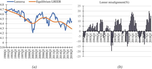
Figure 2(a) shows the actual REER versus the equilibrium (EREER) over the period 1990 to 2018, with the extent of misalignment (expressed as the percentage deviation of the actual REER from the estimated EREER) presented in Figure 2(b). Figure 2 confirms that the exchange rate deviates from its equilibrium level over time with the historical misalignment pattern witnessed confirming similar observations from previous studies including De Jager (2012) and Saayman (2010). The study affirms an extreme undervaluation in the exchange rate in 2001/2002 (about 20% in 2002Q1) and between 2008 and 2009 (about 15% in 2008Q4). A significant correction beginning in 2002 led to the exchange rate to be overvalued by more than 12% by 2006. The REER experienced another episode of undervaluation from 2013Q2 to 2016Q2 with the exchange rate reaching its lowest point of 13% during 2016Q1 which coincided with the removal of the then Minister of Finance, Nhlanhla Nene. Subsequently, the REER has continued to experienced episodes of overvaluation. The plot of the misalignment series (Figure 2(b)) indicates the presence of abrupt changes or shifts in the direction of misalignment and long swings in the deviation of the REER from its equilibrium level. For example, following an undervaluation exceeding 20% in 2002, the exchange rate moved back quickly into equilibrium and was overvalued by about 10% in 2003. Similar moves are observed between 2008 and 2010 when the global financial crisis caused a steep decline in the currency in 2008 before a recovery was observed in 2010.

An analysis of the misalignment series indicates that the exchange rate has been on average more overvalued over the period studied with the series both significantly skewed and leptokurtic. The Jarque–Bera test statistic confirms the departure of the data from normality and provides motivation for the use of a method of analysis with a time-varying component where the current estimates of both the mean and variance of the series are permitted to depend, in some fashion, upon their previous values. As Terra and Valladares (2010) note, a modelling method that identifies whether distinct regimes for misalignment (under- versus overvalued states) exist might provide a better fit for the data (misalignment series). The MSM applied in the study endogenously determines the possible presence of over- and undervaluation episodes that may be regarded as different deviations from the equilibrium exchange rate. Results from the MSM model are presented and discussed below.

Figure 2. Actual versus equilibrium REER and misalignment.

5.3. Markov regime switching model results

In the MSM framework employed, the misalignment series is used as a dependent variable in the model in order to derive the probability of being in a specific regime at a point in time. An important feature of the MSM is to test the hypothesis that the data was generated by a mixture of two normal distributions such that the mean parameters from the different regimes are significantly different. In the current study, the model should account for two states in the misalignment series, namely REER over- and undervaluations. Table 6 presents the results of the MSM and the key parameters of the model which confirm the existence of two exchange rate misalignment episodes.

Table 6. MSM results

Parameter	Estimate	z-Statistic	Prob
µ1	−3.521	−1.741	0.081
µ2	8.699	5.432	0.000
σ^21	1.721	15.207	0.000
σ^22	1.529	12.975	0.000

The estimated parameters confirm that the mean values of the misalignment series are significantly different under the alternative regimes: the state of overvaluation has a positive mean (µ₂ = 8.699) whilst the undervaluation episodes have a negative mean (µ_{1 = −3}.521). The results also confirm that the undervaluation regime has a slightly higher volatility (1.721) than the overvaluation episode (1.529). This should be expected since currency depreciation episodes in South Africa have been mainly abrupt and coincided with significant volatility in the nominal exchange rate. Such a finding is also consistent with the leverage effects that are associated with exchange rate volatility, i.e. negative shocks to the exchange rate lead to higher volatility compared to positive shocks of a similar magnitude (Brooks, 2014).

The probabilities (fixed) of transition from one regime to another are expressed in the matrix below:

P = $\left[\begin{array}{cc}Puu& Puo\\ Pou& Poo\end{array}\right]$ =$\left[\begin{array}{cc}0.90& 0.10\\ 0.09& 0.91\end{array}\right]$

The values of P_uu and P_oo respectively denote the probability of staying in regime 1 (undervaluation) given that the exchange rate was undervalued in the previous quarter, and the probability of staying in regime 2 (overvaluation) given that the exchange rate was in regime 2, respectively. The parameters (P_uu and P_oo) have high values and indicate some stability as they suggest that if the exchange rate is in either regime 1 or 2, it is highly likely to remain in that state in the next period (Pinno & Serletis, 2007). Notable in the MSM results is the higher probability of the exchange rate being overvalued and the fact that overvaluation episodes seem to have on average longer durations (about 11.4 quarters versus 10.3 quarters for undervaluation) over the sample period. This is confirmed when plotting the estimates from the model of the probabilities of being in either of the two regimes over the full sample period.

Figure 3. Probability of being in regime 1 (REER undervalued).

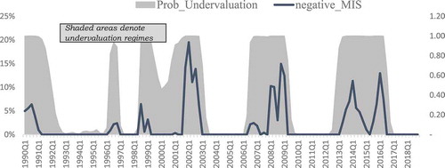
Figures 3 and 4 plot the inferred probabilities (smoothed) from the MSM of being in regimes 1 and 2 and compare such episodes with the misalignment series estimated (solid lines) from the long-run cointegrating relationship. The MSM framework correctly identifies both under- and overvaluation episodes and confirms that the REER was more often overvalued than undervalued in the period 1990–2018. For example, the model confirms the exchange rate was in regime 2 (overvalued) during 1991Q3-1996Q1, 1997Q1-1998Q2, 1999Q2-2000Q4, 2003–2006, 2009Q3–2012Q4 and 20016Q3-2018Q4. Similarly, it correctly tracked when the REER was in regime 1 (undervalued). It is noteworthy that all the episodes of major undervaluations coincided with when there was a crisis either in the domestic economy or externally.

Figure 4. Probability of being in regime 2 (REER overvalued).

6. Concluding remarks and policy implications

Applying the BEER approach, this study finds evidence that a long-run equilibrium relationship exists between the rand’s REER and the terms of trade, external openness, capital flows, investment and government expenditure. Should policymakers wish to use the exchange rate as a policy tool, a key prerequisite is an understanding of the drivers of the equilibrium exchange rate such that any deliberate actions to deal with exchange rate misalignment would have to focus on the underlying fundamentals influencing the exchange rate. The MSM correctly captures the rand’s exchange rate misalignment over the sample period as distinct episodes of over- and undervaluation.

A key finding from the study is the fact that most exchange rate undervaluation episodes have been in response to either idiosyncratic shocks emanating from internal economic challenges (e.g., the rand crisis of 2001) or systemic global factors (2007/2008 global financial crisis) that are transmitted through either the nominal exchange rate or capital flows. These undervaluations have tended to be abrupt and at times extreme with a quick correction and sharp movement to overvaluation such that it cannot be possible for economic agents to make informed decisions based on such exchange rate behaviour. For an undervalued exchange rate to have a macroeconomic impact on exports and economic growth, such misalignment must be policy-induced such that the extreme movements are avoided, which has not been the case in South Africa. On the same note, one can also observe that exchange rate overvaluation episodes have coincided with good economic performance (e.g., between 2003 and 2006). When the economy is performing well, there is sufficient scope for the central bank to initiate policy that will have the effect of weakening the exchange rate in an effort to support long-term export performance. However, such a policy would need to be applied consistently over time for the desired effects to be realised.

correction

This article has been republished with minor changes. These changes do not impact the academic content of the article.

Additional information

Funding

The authors received no direct funding for this research.

Notes on contributors

Meshach Jesse Aziakpono

Meshach Jesse Aziakpono is a Professor of Development Finance at the University of Stellenbosch Business School (USB). Before joining the USB, he was Associate Professor of Economics in the Department of Economics and Economic History at Rhodes University, South Africa. He obtained his PhD degree in Economics from the University of the Free State, Bloemfontein in South Africa. His PhD thesis titled: “The Depth of Financial Integration and its Effects on Financial Development and Economic Performance of the Southern African Customs Union Countries” won the Founders’ Medal for the best PhD dissertation in Economics in South Africa. He has published over 40 papers in international peer-reviewed journals and chapters of books.

Melvin M. Khomo is a General Manager-Financial Markets at the Central Bank of Eswatini (CBE). Before joining the CBE, he was a senior lecturer at the South African Reserve Bank (SARB) Academy. He obtained his PhD in Development Finance from the University of Stellenbosch, South Africa.

Notes

1. MacDonald and Ricci (2004) measure productivity as the log of real GDP relative to South Africa’s trading partners.

2. Other variables considered include the real interest rate differential, money supply, commodity price index, government debt to GDP ratio, foreign exchange reserves and the NEER.

3. This is done by placing a zero restriction on the coefficient of the error correction term corresponding to each variable in the VECM. If the null hypothesis is rejected, then the corresponding variable is not weakly exogenous, hence the variable is treated as endogenous in the model (Luintel & Khan, 1999). If the REER is weakly exogenous, it cannot be used to model the equilibrium exchange rate for the country.

4. The empirical estimation was carried out using EViews 9.5.

5. The speed of adjustment identified in this model of 13% is within the range found in previous studies: De Jager (2012) found 28.50%, MacDonald and Ricci (2004) obtained 8%.

6. The coefficients of error correction term in the VECM for the variables and the corresponding t-statistic in brackets are −0.127(−2.64); −0.036(−1.135); 0.43(4.09); 0.073(2.33); 0.003(0.101) and 0.017(0.37) respectively for LREER, LTOT, CAP, LOPEN, LINV and LGOV.

References

- Aflouk, N., Jeong, S.-E., Mazier, J., & Saadaoui, J. (2010). Exchange rate misalignments and international imbalances: A FEER approach for emerging countries. International Economics, 124, 31–16. https://doi.org/10.1016/S2110-7017(13)60019-0
- Ajevskis, V., Rimgailaite, R., Rutkaste, U., & Tkacevs, O. (2012). The assessment of equilibrium real exchange rate of Latvia. Latvijas Banka Working Paper 04/2012. Retrieved 17 July 2016 www.m.bank.lv
- Aron, J., Elbadawi, I., & Kahn, B. (1997). Determinants of the real exchange rate in South Africa. Working Paper Series WPS/97–16. Centre for the Study of African Economies, University of Oxford, London, April.
- Baak, S. (2012). Measuring misalignments in the Korean exchange rate. Japan and the World Economy, 24(4), 227–234. https://doi.org/10.1016/j.japwor.2012.09.001
- Bazdresch, S., & Werner, A. (2005). Regime switching models for the Mexican peso. Journal of International Economics, 65(1), 185–201. https://doi.org/10.1016/j.jinteco.2004.02.002
- Brooks, C. (2014). Introductory Econometrics for Finance (3rd ed.). Cambridge University Press.
- Brooks, C., & Persand, G. (2001). The trading profitability of forecasts of the gilt-equity yield ration. International Journal of Forecasting, 17(1), 11–29. https://doi.org/10.1016/S0169-2070(00)00060-1
- Clark, P. B., & MacDonald, R. (1998). Exchange rates and economic fundamentals: A comparison of BEERs and REERs. IMF Working Paper No. 98/67.
- De Jager, S. (2012). Modelling South Africa’s equilibrium real effective exchange rate: A VECM approach. Working Paper WP/12/02. South African Reserve Bank.
- Du Plessis, S. A. (2005). Exogeneity in a recent exchange rate model: A response to MacDonald and Ricci. South African Journal of Economics, 73(4), 741–746. https://doi.org/10.1111/j.1813-6982.2005.00050.x
- Eita, J. H., & Sichei, M. M. (2006). Estimating the equilibrium real exchange rate for Namibia. Working Paper 2006-8. University of Pretoria, Department of Economics.
- Elbadawi, I., Kaltani, L., & Soto, R. (2012). Aid, real exchange rate misalignment, and economic growth in Sub-Saharan Africa. World Development, 40(4), 681–700. https://doi.org/10.1016/j.worlddev.2011.09.012
- Engel, C. (1994). Can the Markov switching model forecast exchange rates? Journal of International Economics, 36(1–24), 151–165. https://doi.org/10.1016/0022-1996(94)90062-0
- Engel, C., & Hamilton, J. D. (1990). Long swings in the dollar: Are they in the data and do markets know it? American Economic Review, 80(4), 689–713. https://www.jstor.org/stable/2006703
- Gan, C., Ward, B., Ting, S. T., & Cohen, D. A. (2013). An empirical analysis of China’s equilibrium exchange rate: A co-integration approach. Journal of Asian Economics, 29 (issue C), 33–44. https://doi.org/10.1016/j.asieco.2013.08.005
- Goldfajn, I., & Valdés, R. O. (1999). The aftermath of appreciations. The Quarterly Journal of Economics, 114(1), 229–262. https://doi.org/10.1162/003355399555990
- Guo, H., Brooks, R., & Shami, R. (2010). Detecting hot and cold cycles using a Markov regime switching model—Evidence from the Chinese A-share IPO market. International Review of Economics and Finance, 19(2), 196–210. https://doi.org/10.1016/j.iref.2009.10.002
- Hamilton, J. D. (1989). A new approach to the economic analysis of nonstationary time series and the business cycle. Econometrica, 57(2), 357–384. https://doi.org/10.2307/1912559
- Hossfeld, O. (2010). Equilibrium real effective exchange rates and real exchange rate misalignments: Time series vs. panel estimates. FIW Working paper Series 065, FW.
- Johansen, S. (1995). Likelihood-based inference in cointegrated vector autoregressive models. Oxford University Press.
- Korsu, R. D., & Braima, S. J. (2011). The determinants of the real exchange rate in Sierra Leone. China-USA Business Review, 10(9), 745–762. doi: 10.17265/1537-1514/2011.09.002
- Lòpez-Villavicencio, A., Mazier, J., & Saadaoui, J. (2012). Temporal dimension and equilibrium exchange rate: A FEER/BEER comparison. Emerging Markets Review, 13(1), 58–77. https://doi.org/10.1016/j.ememar.2011.10.001
- Luintel, K. B., & Khan, M. (1999). A quantitative reassessment of the finance-growth nexus: Evidence from a multivariate VAR. Journal of Development Economics, 60(2), 381–405. https://doi.org/10.1016/S0304-3878(99)00045-0
- MacDonald, R., & Ricci, L. A. (2004). Estimation of the equilibrium real exchange rate for South Africa. South African Journal of Economics, 72(2), 282–304. https://doi.org/10.1111/j.1813-6982.2004.tb00113.x
- MacDonald, R., & Ricci, L. A. (2005). Exogeneity in a recent exchange rate model: A reply. South African Journal of Economics, 73(4), 747–753. https://doi.org/10.1111/j.1813-6982.2005.00051.x
- MacKinnon, J. G., Haug, A. A., & Michelis, L. (1999). Numerical distribution functions of likelihood ratio tests for cointegration. Journal of Applied Econometrics, 14(5), 563–577. https://doi.org/10.1002/(SICI)1099-1255(199909/10)14:5<563::AID-JAE530>3.0.CO;2-R
- Maitland-Smith, J., & Brooks, C. (1999). Threshold autoregressive and Markov switching models: An application to commercial real estate. Journal of Property Research, 16(1), 1–19. https://doi.org/10.1080/095999199368238
- Nikolsko-Rzhevskyy, A., & Prodan, R. (2012). Markov switching and exchange rate predictability. International Journal of Forecasting, 28(2), 353–365. https://doi.org/10.1016/j.ijforecast.2011.04.007
- Palić, I., Dumičić, K., & Šprajaček, P. (2014). Measuring real exchange rate misalignment in Croatia: Cointegration approach. Croatian Operational Research Review, 135(5), 135–148. https://doi.org/10.17535/crorr.2014.0003
- Perron, P. (2006). Dealing with structural breaks. In K. Patterson & T. C. Mills (Eds.), Palgrave Handbook of Econometrics, Vol 1: Econometric Theory (pp. 278–352). Palgrave Macmillan.
- Pinno, K., & Serletis, A. (2007). Long swings in the Canadian Dollar. Applied Financial Economics, 15(2), 73–76. https://doi.org/10.1080/0960310042000282292
- Rangasamy, L. (2009). Exports and economic growth: The case of South Africa. Journal of International Development, 21(5), 603–617. https://doi.org/10.1002/jid.1501
- Saayman, A. (2007). The real equilibrium South African rand/US dollar exchange rate: A comparison of alternative measures. International Advances in Economic Research, 13(2), 183–199. https://doi.org/10.1007/s11294-006-9075-6
- Saayman, A. (2010). A panel data approach to the behavioural equilibrium exchange rate of the ZAR. South African Journal of Economics, 78(1), 57–75. https://doi.org/10.1111/j.1813-6982.2010.01232.x
- Saikkonen, P. (1992). Estimation and testing of cointegrated systems by an autoregressive approximation. Econometric Theory, 8(1), 1–27. https://doi.org/10.1017/S0266466600010720
- Stock, J. H., & Watson, M. W. (1993). A simple estimator of cointegrating vectors in higher order integrated systems. Econometrica, LXI(4), 783–820. https://doi.org/10.2307/2951763
- Terra, C., & Valladares, F. (2010). Real exchange rate misalignments. International Review of Economics and Finance, 19(1), 119–144. https://doi.org/10.1016/j.iref.2009.05.004