Firm age and crude oil returns: Stock price sensitivity of oil-producing and consuming companies

Abstract

This study aims to identify firm characteristics that affect the cross-firm variation in oil–stock interactions. A panel data analysis with a sample of U.S. and Canadian firms reveals that the stock price sensitivity to crude oil price returns is negatively and significantly associated with firm age. Contrary to a common belief, firm size or stock liquidity does not seem to influence heterogeneity in oil–stock relationships. My finding is consistent across oil-producing and consuming companies while the effect of firm age is not observed among financial institutions engaged in commodity trading. An additional test using the panel Granger causality approach shows no lagged effect of oil market movement on the oil and gas extraction firms, suggesting their prompt response to market information.

Keywords:

• Crude oil price
• stock returns
• firm age
• panel causality

GEL Classification:

• C32
• G12
• G13

PUBLIC INTEREST STATEMENT

The valuation of a young firm is often challenging due to a limited earnings history coupled with seemingly unlimited growth potential. This article shows that the stock prices of young oil-producing and consuming companies are more sensitive to changes in the crude oil market than their more mature counterparts. My analysis also confirms that the stock returns of these firms respond to oil market movement without delay. Combined, these findings suggest that investors place a heavier weight on market-wide information when assessing a young firm, and such information is quickly reflected in stock valuations. My study offers useful implication for today’s investors, who manage portfolios including a wide range of asset classes beyond traditional stocks and fixed-income securities.

1. Introduction

The development of the oil price is one of the macroeconomic factors common to all firms yet heterogeneous in effect. This article investigates how changes in the crude oil price affect stock prices at the firm level and whether variation in oil–stock relationships is associated with specific firm characteristics. These questions are worthy of investigation as the impact of oil price movement is among the issues of utmost relevance to economy and businesses. For example, Hamilton (1983) indicates that increases in the crude oil price preceded the most of the recessions in the U.S. between 1948 and 1972. A more recent study by Kilian and Park (2009) suggests that approximately 22% of the variation in U.S. stock returns between 1975 and 2006 is attributable to the fundamental shocks in oil demand and supply.¹ In addition, today’s investors manage portfolios including a wide range of asset classes beyond traditional stocks and fixed-income securities (Singleton, 2014; Tang & Xiong, 2012). Understanding the dynamics between stock and commodity prices is increasingly more important for us.

Earlier studies on the impact of the oil price on financial markets focus on broad-based market indexes, where the causality test based on Granger’s (1969) approach is typically adopted (e.g., Huang et al., 1996; Jones & Kaul, 1996; Sadorsky, 1999). Sector-level analyses are also introduced in later studies, and the standard market model augmented by the oil price factor is commonly used (e.g., Boyer & Filion, 2007; El-Sharif et al., 2005; Mohanty & Nandha, 2011; Sadorsky, 2001). Although these studies provide useful insight in market dynamics from macro perspectives, they do not necessarily answer my specific research questions.² The lack of attention to the cross-firm heterogeneity in literature motivates me to conduct an analysis with firm-level granularity.

This study utilizes the panel data regression models to analyze the contemporaneous association between the oil–stock relationship and firm characteristics. The firm-specific attributes examined are firm age, firm size, liquidity of a firm’s stock, and a firm’s sensitivity to the overall equity market. The dynamic, or lagged, effect of oil price returns on stock prices is examined using the Dumitrescu and Hurlin (2012) panel Granger causality test. Due to its small-sample properties and relative simplicity, the Dumitrescu-Hurlin test has gained popularity in recent financial studies (e.g., Naik & Padhi, 2015; Shahbaz et al., 2015 among others).

The value of a firm’s stock is theoretically equal to the sum of its discounted future cash flows. If the firm’s operations are vulnerable to changes in energy markets, its stock valuation should be linked to the crude oil or natural gas prices more directly. Accordingly, much of the previous work on oil-stock linkages specifically examines the oil and gas industries (e.g., El-Sharif et al., 2005; Gupta, 2016; Mohanty & Nandha, 2011; Ramos & Veiga, 2011; Sadorsky, 2001). Following these studies, my analysis mainly focuses on oil and gas extraction companies. Limiting the scope of the study to relevant industries, instead of covering all the sectors, is meaningful because the purpose of this paper is to conduct an in-depth analysis at the firm level. For a comparison purpose, I also include other firms closely related to energy prices: petroleum products manufacturing, electric and gas utilities, and transportation. The selection of firms in this study is consistent with Bartov et al. (1996), which define the “oil-price sensitive firms” to control for influences of oil price shock. Lastly, the financial institutions engaged in commodity trading activities are added to the analysis.

The present article makes a twofold contribution. First, this study extends literature by examining the linkage between the returns of the crude oil price and stock prices at the firm level. A pretest using a multifactor asset pricing model suggests that the NYMEX WTI light sweet crude oil (NYMEX/WTI) futures contract price returns significantly impact the returns of the overwhelming majority of the oil-price sensitive firms in the U.S. and Canada. While this is consistent with the previous research, my study further adopts the panel regression analysis to identify the firm characteristics that affect the oil–stock interactions.

Second, this study connects two strands of literature, firm age and oil-stock linkages, which seem to have developed separately despite their relevance to each other. The panel regression analysis in this article reveals that young firms are more sensitive to the oil price movement than their more mature counterparts. My finding accords with the notion that the valuation of a younger firm is more subjective and difficult to arbitrage due to a limited earnings history coupled with seemingly unlimited growth potential (Baker & Wurgler, 2006; Chen et al., 2019). I believe that such challenge results in investors placing a greater weight on market-wide information when assessing a young firm.

The remainder of this paper is organized as following. Section 2 reviews the literature on the oil–stock interactions and the effect of firm age in investor decisions from various perspectives. Section 3 presents descriptive statistics of data. Section 4 describes the methodology used in my analysis and the empirical results on firm characteristics affecting variation in the contemporaneous as well as lagged effects of the oil price on stock returns. Section 5 provides concluding remarks.

2. Related literature

2.1. Oil-stock relationships

The pivotal role of oil prices in economy has prompted a volume of literature investigating the linkages between crude oil prices and macroeconomic variables (e.g., Hamilton, 1983; Hooker, 1996). Since the seminal work by Jones and Kaul (1996), empirical studies on the causal link between the oil prices and financial markets have burgeoned. Using the Producer Price Index for fuels as a proxy of the oil price, Jones and Kaul (1996) report that stock returns in the U.S. and Canada were negatively impacted by oil prices. In contrast, Huang et al. (1996) find no evidence of a causal relationship between crude oil futures price returns and the broad-based market returns, except in the case of oil companies. Using the U.S. industrial output data, interest rate, and real oil prices, Sadorsky (1999) concludes that the increase in the oil price negatively affects stock returns in the U.S. while stock returns positively impact the interest rate and industrial output.

While earlier studies focus on the effect of the oil price on broad-market indexes, more recent research recognizes cross-sector heterogeneity in stock market sensitivity and conducts empirical tests at the sector level. For example, Sadorsky (2001) concludes that oil and gas stock prices are positively affected by the increase in the oil price as well as increases in the broad-based market indexes. Likewise, Boyer and Filion (2007) suggest that the energy stock returns are positively associated with crude oil and natural gas prices and negatively associated with interest rates. Focusing on the alternative energy companies, Henriques and Sadorsky (2008) show that technology stock prices and crude oil prices individually impact alternative energy stocks.

Researchers have also analyzed the oil-stock causal link using the data from the regions other than the North America. El-Sharif et al. (2005) report positive relationship between oil price return and energy-stock returns in the United Kingdom. Nandha and Faff (2008) analyze 35 industry sectors globally and show that the stock price returns are negatively impacted by increases in oil prices with the exception of mining, oil and natural gas industries. Arouri and Nguyen (2010) examine short-term linkages in the sector-by-sector levels in Europe and suggest that there is either unidirectional or bidirectional causality between the stock price returns and oil price changes, depending on the sector.³ Ramos and Veiga (2011) report that oil and gas stocks in developed countries respond more strongly to oil price changes than those in developing countries. Regardless of the country or region, virtually all of the sector-level studies share a common conclusion; oil price changes positively affect the aggregate returns of oil and gas industries while negative association is observed for other industries. This is quite reasonable because the revenues of energy firms heavily depend on the price levels of oil and natural gas. Conversely, increases in energy prices mean higher costs for the firms in other industries.

Relatively little statistical work has been done to investigate the oil–stock interactions with firm-level granularity. While none of the extent studies to my knowledge explicitly examines firm age as a factor possibly affecting the oil–stock relationships, some studies report significant effect of firm size. For example, Narayan and Sharma (2011) show that the contemporaneous effect of oil prices is stronger on large-company stocks than small-company stocks while lagged effect of oil price returns is not associated with specific firm characteristics. Analyzing bidirectional oil–stock relationships, Lv et al. (2020) indicate that the stock returns of large petrochemical companies in the U.S. and China have positive impact on oil price movement while those of smaller firms do not.

Country and industry-level factors likewise affect the oil–stock relationship at the firm level. For example, Kang et al. (2017) examine seven major integrated oil and gas companies, and show that the effect of oil price shocks on stock returns are amplified by shocks to economic policy uncertainty. Similarly, a research by Gupta (2016) indicates that the stock returns of the oil and gas companies operating in competitive industries or located in high oil-producing countries are more sensitive to oil price shocks.

2.2. Effect of firm age

As stated earlier, this article aims to bridge two strands of literature: oil-stock linkages and firm age. Although I specifically focus on the crude oil price as the source of market information, there exists a number of studies analyzing the relationships between firm age and investor decisions from various perspectives. In general, it is more difficult for investors to assess younger firms due to adverse selection problems. Morellec and Schürhoff (2011) suggest that a young firm lacks established relations with capital markets and therefore suffers from higher cost of external financing. In contrast, Pástor and Veronesi (2003) report that young firms’ market-to-book ratios can be overvalued due to uncertainty about their future profitability.

One way to observe the effect of firm age more directly is to examine whether the stocks of young and mature firms show different reactions to macroeconomic factors. It is widely known that firm age is closely related with the impact of market sentiment on investor decisions. That is, the effect of investor sentiment tends to be stronger for younger firms than mature firms (Baker & Wurgler, 2006; Chen et al., 2019). Mian and Sankaraguruswamy (2012) suggest that strong stock responses to earnings reports during high sentiment periods are even more pronounced for younger stocks. A similar research by Vieira (2011) shows that the impact of investor sentiment to the stock reaction to dividend-change announcements is greater for a younger firm in the UK. Investor sentiment also affects the timing of a firm issuing seasoned equity. Chen et al. (2019) show that a young firm is more likely to issue equity when market sentiment is high.

Studies show that firm age also influences analyst forecasts. For example, it is known that there is a close relationship between firm age and forecast revision timeliness. Jennings et al. (2017) show that analysts revise earnings-per-share forecasts more quickly for younger firms, firms with higher institutional ownership, and firms with lower ROAs. Similarly, Griffin et al. (2020) report that forecast revisions occur more frequently for younger firms and firms with less corporate social responsibility (CSR) disclosure. Moreover, Ertimur et al. (2011) show that analysts are more likely to produce disaggregated revenue estimates for young firms. One implication from these findings is that investors expect analysts to provide more detailed and frequently updated information with respect to younger firms. This view provides an additional explanation for the empirical result in this paper that the stock returns of young oil-producing and consuming companies are more responsive to market-wide news.

3. Data

3.1. Industry classifications and scope of the analysis

The firms are selected based on the classifications by the North American Industry Classification System (NAICS). Since 1997, the NAICS has been adopted by federal statistical agencies to replace the Standard Industrial Classification (SIC) system. As stated in Section 1, the primary focus of this study is the effect of oil price returns on the oil and gas extraction firms, for which the first four digits of the NAICS code are 2111. The U.S. Bureau of Labor Statistics explains that the operations of a firm in this sector involve “exploration for crude petroleum and natural gas, drilling, completing, and equipping wells, operating separators, emulsion breakers, desilting equipment, and field gathering lines for crude petroleum and natural gas, and all other activities in the preparation of oil and gas up to the point of shipment from the producing property.” The future cash flows of an extraction company can be directly impacted by oil price movement. For convenience, this industry is referred to as “Group #1” throughout the rest of the paper.

Our analysis also includes other oil-price sensitive industries, in which firm’s operations are closely related to energy prices. These include the utilities associated with electric power generation, transmission, and distribution (NAICS: 2211), the utilities that operate natural gas distribution (NAICS: 2212), and the petroleum products manufacturing (NAICS: 3241). Some of them are vertically integrated oil and gas companies with highly diversified lines of business (e.g., ExxonMobil), where a firm’s investment opportunity may not be impacted significantly by the oil price return alone. All the transportation firms, including the pipeline firms for crude oil (NAICS: 4861) and natural gas (NAICS: 4862), are included. To avoid a small-sample issue, these industries are combined into one group and tested together. They are collectively referred to as “Group #2” in the remainder of the paper.

The third group examined consists of the financial institutions that possibly trade energy derivatives (e.g., crude oil futures). These firms are found in the securities and commodity contracts intermediation and other financial investments and related activities (NAICS: 523).⁴ Due to the speculative nature of their involvement in energy markets, the firms in this sub-sector are tested separately as “Group #3.” With Groups #1, #2, and #3 combined, the data associated with a total of 660 firms are collected. All of these firms are headquartered in the U.S. or Canada.

3.2. Data collection and summary statistics

This study utilizes U.S. crude oil futures and stock market data observed between January 2007 and December 2019. This particular period covers one economic cycle including the financial crisis of 2007–2008, the most recent economic recession that the U.S. economy experienced. The daily prices of the NYMEX/WTI futures contract were obtained from the Energy Information Administration (EIA) of the U.S. Department of Energy. Following Fama and French (1987), a continuous series of the NYMEX/WTI futures price is constructed using the nearest-to-delivery contracts. The daily stock prices of individual firms come from the Center for Research in Security Prices (CRSP). The financial statement data are collected from the Compustat North America database.

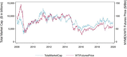
Table 1 summarizes the daily price of the NYMEX/WTI futures contract (Panel A) and the value-weighted daily stock price return of the oil and gas extractives sector (Panel B), both between January 2007 and December 2019. For intuitiveness, Panel A presents the crude oil price level (in U.S. dollars) instead of the percentage return. Figure 1 provides visual representation of the time series of these variables in slightly different ways. The left axis of the chart indicates the level of the total market capitalizations (in billions of dollars) consisting of the oil and gas extractives firms while the right axis indicates the price level (in dollars) of the nearest-to-delivery NYMEX/WTI futures contract. All the data are on a daily basis. At a glance, these markets overall appear to have moved in tandem during most of the sample period, except during the period of market turmoil in 2008.

Table 1. Crude oil price and value-weighted return of oil and gas extractives firms

Panel A: Daily NYMEX/WTI Futures Price Level ($/Bbl)
Year	2008	2009	2010	2011	2012	2013	2014	2015	2016	2017	2018	2019
Min	33.87	33.98	68.01	75.67	77.69	86.68	53.27	34.73	26.21	42.53	42.53	46.54
Max	145.29	81.37	91.51	113.93	109.77	110.53	107.26	61.43	54.06	60.42	76.41	66.30
Mean	99.75	62.09	79.61	95.11	94.15	98.05	92.91	48.79	43.40	50.80	64.81	57.07
Std. Dev.	28.42	13.36	5.19	8.08	7.68	5.43	13.37	6.81	6.72	3.88	6.81	3.70
Panel B: Daily Value-Weighted Stock Price Return of the Oil and Gas Extractives (%)
Year	2008	2009	2010	2011	2012	2013	2014	2015	2016	2017	2018	2019
Min	-15.7%	-10.6%	-5.5%	-8.9%	-5.9%	-5.0%	-7.2%	-8.6%	-6.2%	-3.9%	-5.4%	-4.8%
Max	24.3%	12.1%	6.5%	8.2%	6.4%	4.9%	6.3%	15.2%	6.5%	3.7%	5.6%	8.4%
Mean	-0.1%	0.2%	0.2%	-0.1%	0.1%	0.0%	-0.1%	-0.1%	0.1%	0.1%	0.0%	0.1%
Std. Dev.	4.9%	3.1%	2.1%	2.6%	1.8%	1.4%	1.6%	2.4%	2.1%	1.1%	2.1%	1.6%

Panel A shows the summary of the daily quoted price level (in dollar) of the nearest-to-delivery NYMEX/WTI futures contract during each year between January 2008 and December 2019. Panel B shows the summary of the value-weighted daily stock price return of the firms in the oil and gas extraction sub-sector during the same period.

Figure 1. Crude oil price and market capitalization of oil and gas extractives firms

The left axis of the chart indicates the daily level of the aggregated market capitalizations (in billions of dollars) consisting of the firms in the oil and gas extraction sub-sector between January 2008 and December 2019. Market capitalization for each firm is determined as the number of common shares outstanding multiplied by the share price. The right axis indicates the daily price level (in dollars) of the nearest-to-delivery NYMEX/WTI futures contract during the same period.

The series of weekly log differences (i.e., log returns) are constructed based on the daily stock prices of an individual firms and the NYMEX/WTI futures price, observed on the same day. The weekly data were retrieved from every Tuesday; if Tuesday was not available (e.g., non-trading day), then Wednesday was used. If both Tuesday and Wednesday were unavailable, then Monday is used. This strategy ensures that each price change is encompassed about seven days.⁵ The purpose of this article is to investigate idiosyncratic firm characteristics that may contribute to the variation in the oil–stock relationships. These firm-specific variables are following:

1. Firm age: As a proxy of a firm’s age, I obtained the number of years the firm has been listed in CRSP.

2. Firm size: A firm’s market capitalization is determined as the average of the firm’s share price multiplied by the number of common shares outstanding.

3. Stock liquidity: The average of a firm’s daily transaction volumes during the sample period is calculated. I believe that the transaction volume effectively measures the liquidity of the stock issued by each firm.

4. Systematic risk: This variable is included to incorporate the variation in stock return sensitivity to the overall market, and I use the average of a firm’s beta on the excess return on the market during the sample period as a proxy. Following Fama and French (1993), the market return is determined as the CRSP value-weighted stock returns. The market beta of each firm was estimated with a 252-day window.

Table 2 presents the summary of the firm-specific variables observed during the sample period, sorted by the group of industries described in Section 1. In order to create a balanced panel dataset, the firms included in this study must have accounting and stock price information for the entire sample period. This automatically eliminates the firms that have been listed in CRSP for less than 13 years, reducing the number of firms to 243.

Table 2. Summary of firm-specific characteristics by group

Panel A: Oil and gas extraction
	Number of firms	Min	Max	Mean	Std. Dev.
Firm’s age	56	13	95	30.15	19.16
Market capitalization ($ in million)	56	5	82,100	9,050	15,200
Stock liquidity (shares in thousand)	56	2	23,500	2,672	3,783
Beta on market return	56	0.419	2.036	1.353	0.365
Panel B: Petroleum, electric and gas utilities, and transportation
	Number of firms	Min	Max	Mean	Std. Dev.
Firm’s age	119	13	95	44.29	24.64
Market capitalization ($ in million)	119	14	375,000	14,700	39,500
Stock liquidity (shares in thousand)	119	3	18,300	1,820	2,644
Beta on market return	119	0.145	2.118	0.924	0.390
Panel C: Securities and commodity contracts intermediation
	Number of firms	Min	Max	Mean	Std. Dev.
Firm’s age	68	13	83	25.90	14.02
Market capitalization ($ in million)	68	21	74,900	6,630	13,400
Stock liquidity (shares in thousand)	68	6	16,600	1,584	3,329
Beta on market return	68	0.319	1.984	1.216	0.373

Statistics are based only on the firms that have stock price information for the entire sample period. Firm’s age is the number of years firm i had been listed in CRSP as of 2019 or at the time when the firm was delisted from CRSP, and its minimum value is 13. The other values are averages during the sample period, January 2007—December 2019: Market capitalization is the number of common shares outstanding multiplied by the daily share price; Stock liquidity indicates firm i’s daily transaction volume; and Beta on market return is firm i’s beta to the CRSP value-weighted stock returns.

As presented in Table 3, the correlation coefficients of the variables within each of Groups #1, #2, and #3 are relatively low. To ensure the validity of the regression results, I also check the presence of multicollinearity among these variables. Based on the variance inflation factors (VIFs) shown in the sixth column of Table 3, I conclude that multicollinearity is not present in any of the subgroups. For example, Panel A (i.e., Group #1) shows that the VIFs for the variables in the model range from 1.30 to 2.92, which is substantially below the widely accepted threshold.

Table 3. Correlations and variance inflation factors of firm characteristics

Panel A: Oil and gas extraction
Variable	Firm’s age	Size (ln)	Liquidity (ln)	Beta	VIF
Firm’s age	1				1.30
Firm’s size (ln)	0.312	1			2.92
Stock liquidity (ln)	0.188	0.787	1		1.30
Beta	-0.231	0.357	0.406	1	1.40
Panel B: Petroleum, electric and gas utilities, and transportation
Variable	Firm’s age	Size (ln)	Liquidity (ln)	Beta	VIF
Firm’s age	1				1.55
Firm’s size (ln)	0.433	1			3.92
Stock liquidity (ln)	0.342	0.821	1		3.92
Beta	-0.459	-0.201	0.077	1	1.62
Panel C: Securities and commodity contracts intermediation
Variable	Firm’s age	Size (ln)	Liquidity (ln)	Beta	VIF
Firm’s age	1				1.03
Firm’s size (ln)	0.034	1			3.53
Stock liquidity (ln)	-0.059	0.835	1		3.50
Beta	0.034	0.540	0.529	1	1.46

The table shows the correlation coefficients and the variance inflation factors (VIFs) calculated based on the data between January 2007 and December 2019. Firm’s age is the number of years firm i had been listed in CRSP as of 2019 or at the time when the firm was delisted from CRSP. Firm’s size is the natural logarithm of firm i’s market capitalization (number of common shares outstanding multiplied by the daily share price). Stock liquidity indicates the natural logarithm of firm i’s daily transaction volume. Beta on market return is firm i’s beta to the CRSP value-weighted stock returns.

3.3. Unit root tests

In order to perform an analysis with a vector autoregressive (VAR) framework, all the time-series data involved in the system must be integrated of the same order. The order of integration of each time series was examined using the augmented Dickey and Fuller (1979, ADF) test. The ADF test is a one-sided left tail test and its null hypothesis is rejected if the test statistic is below the critical value for the intended confidence interval. The Phillips and Perron (1988, PP) test was also performed as an alternative method. In both the ADF and the PP tests, rejecting the null hypothesis means that a variable is stationary.⁶

The results of the unit-root tests on the weekly crude oil and the stock prices, in levels and with log differences, are reported in Table 4. The table also includes the unit-root test results on the value-weighted weekly returns of the S&P 500 Index during the same period. Although it is customary to include first-differenced values in a unit root test, this study instead examines the log differences (i.e., log returns) of prices as they are of more relevance to this study. Due to a large number of the firms involved, the table only includes one firm from each industry.

Table 4. Unit root tests on crude oil futures prices, S&P 500 index, and select stocks

			ADF Test		PP Test
Index/Firm	Case	Obs.	Levels	Returns	Levels	Returns
NYMEX/WTI futures price	no trend	676	-2.000	-18.620**	-2.119	-26.287**
	w/ trend	676	-2.565	-18.629**	-2.645	-26.282**
S&P 500 Index	no trend	676	0.800	-18.430**	0.922	-28.384**
	w/ trend	676	-2.306	-18.422**	-2.249	-28.370**
Harvest Oil & Gas Corp.	no trend	676	-0.523	-18.750**	-0.597	-28.018**
	w/ trend	676	-1.378	-18.994**	-1.414	-28.441**
Exxon Mobil Corp.	no trend	676	-2.795	-20.396**	-2.736	-28.218**
	w/ trend	676	-2.727	-20.403**	-2.663	-28.233**
American Electric Power Co.	no trend	676	0.887	-19.224**	0.898	-27.389**
	w/ trend	676	-1.632	-19.286**	-1.662	-27.444**
SkyWest, Inc.	no trend	676	0.399	-17.606**	0.519	-26.343**
	w/ trend	676	-1.466	-17.667**	-1.328	-26.411**

The unit-root test is conducted with weekly price returns between January 2007 and December 2019. The values shown are the augmented Dickey-Fuller (ADF) and the Phillips-Perron (PP) test statistics both determined with the lag length of 1. The levels of S&P 500 Index indicates the total market values. The levels of the other variables are the quoted prices. The asterisks represent the significance level of 1% (**) and 5% (*).

Based on both the ADF and the PP tests, the NYMEX/WTI futures price, the S&P 500 Index, and the prices of all the stocks listed in this table are shown to be non-stationary in levels. The unit root tests on the rest of the firms overall indicate similar results.⁷ When the tests are performed on the log return series, the null hypothesis of non-stationarity is rejected at the significance level of 1% with respect to the NYMEX/WTI futures price, the S&P 500 Index, and the prices of all the individual stocks. The test statistics shown in the table are determined with one additional lag of the first-differenced variable (the ADF test) or one Newey-West lag (the PP test). Nevertheless, the test results are robust to different lag-length specifications as well as the inclusion of a time trend. All the regression tests in the subsequent section are conducted using the log returns.

4. Methodology and empirical results

4.1. Firm characteristics and stock sensitivity to oil price returns

Most of the studies outlined in Section 2 involve country- or sector-level analyses showing positive effect of oil price changes on the returns of oil and gas companies as a whole. In contrast, this study examines the impact of oil price movement at the individual-firm level. To investigate the association between firm characteristics and the stock price sensitivity to the oil market, the following panel regression model is implemented.

(1) $\begin{array}{rl}& \mathrm{R}{\left(\mathrm{i}\right)}_t={\beta }_0+{\beta }_1{\mathrm{M}}_t+{\beta }_2{\mathrm{O}}_t\\ & +{\beta }_3{\mathrm{O}}_t\times {\mathrm{D}}_{\mathrm{L}\mathrm{o}\mathrm{w}}\left(\mathrm{i}\right)+{\beta }_4{\mathrm{O}}_t\times {\mathrm{D}}_{\mathrm{M}\mathrm{i}\mathrm{d}}\left(\mathrm{i}\right)+{\beta }_5{\mathrm{O}}_t\times {\mathrm{D}}_{\mathrm{H}\mathrm{i}\mathrm{g}\mathrm{h}}\left(\mathrm{i}\right)+\alpha \left(\mathrm{i}\right)+{\delta }_t+{\epsilon }_i\end{array}$(1)

$\mathrm{R}{\left(i\right)}_t$ represents the return of stock i at time t. This is regressed on two different financial determinants: the value-weighted S&P 500 Index return denoted by ${\mathrm{M}}_t$ and the NYMEX/WTI futures contract price return, ${\mathrm{O}}_t$, both at time t. Earlier studies postulate that the crude oil price is driven predominantly by exogenous events specific to the energy sector (e.g., OPEC embargoes), implying that oil price shocks precede virtually all economic variables (Hamilton, 1983; Jones & Kaul, 1996). However, more recent studies suggest that both the crude oil and stock markets have been driven by some of the same economic factors (Barsky & Kilian, 2001; Hamilton, 2003). Equation (1)(1) $\begin{array}{rl}& \mathrm{R}{\left(\mathrm{i}\right)}_t={\beta }_0+{\beta }_1{\mathrm{M}}_t+{\beta }_2{\mathrm{O}}_t\\ & +{\beta }_3{\mathrm{O}}_t\times {\mathrm{D}}_{\mathrm{L}\mathrm{o}\mathrm{w}}\left(\mathrm{i}\right)+{\beta }_4{\mathrm{O}}_t\times {\mathrm{D}}_{\mathrm{M}\mathrm{i}\mathrm{d}}\left(\mathrm{i}\right)+{\beta }_5{\mathrm{O}}_t\times {\mathrm{D}}_{\mathrm{H}\mathrm{i}\mathrm{g}\mathrm{h}}\left(\mathrm{i}\right)+\alpha \left(\mathrm{i}\right)+{\delta }_t+{\epsilon }_i\end{array}$(1) therefore includes the S&P 500 Index return as a proxy of the overall market performance.⁸

In addition, Equation (1)(1) $\begin{array}{rl}& \mathrm{R}{\left(\mathrm{i}\right)}_t={\beta }_0+{\beta }_1{\mathrm{M}}_t+{\beta }_2{\mathrm{O}}_t\\ & +{\beta }_3{\mathrm{O}}_t\times {\mathrm{D}}_{\mathrm{L}\mathrm{o}\mathrm{w}}\left(\mathrm{i}\right)+{\beta }_4{\mathrm{O}}_t\times {\mathrm{D}}_{\mathrm{M}\mathrm{i}\mathrm{d}}\left(\mathrm{i}\right)+{\beta }_5{\mathrm{O}}_t\times {\mathrm{D}}_{\mathrm{H}\mathrm{i}\mathrm{g}\mathrm{h}}\left(\mathrm{i}\right)+\alpha \left(\mathrm{i}\right)+{\delta }_t+{\epsilon }_i\end{array}$(1) incorporates firm characteristics in the form of tercile dummies. Specifically, each of the dummy variables indicates whether firm i is within the bottom one-third (young firm, small firm, low stock liquidity, or low beta), the middle one-third, and the top one-third (mature firm, large firm, high stock liquidity, or high beta) within a subgroup. For example, ${\mathrm{D}}_{\mathrm{L}\mathrm{o}\mathrm{w}}\left(i\right)$ with respect to firm age takes on a value of 1 if firm i is within the bottom one-third in terms of the number of years since its first appearance in CRSP (i.e., relatively young within its subgroup). Each of the interaction terms is a multiple of ${\mathrm{O}}_t$ and one of the tercile dummies. $\alpha \left(\mathrm{i}\right)$ contains a set of firm-specific fixed effects to capture the unobserved, time-invariant heterogeneity. In addition, ${\delta }_t$ represents year fixed effects as I exercise caution with macroeconomic impact common to all firms in a given year.⁹

The result of the panel regression analysis is reported in Table 5. Panels A, B, and C correspond to Groups #1, #2, and #3 defined in Section 3, respectively. Returns are on a weekly basis.¹⁰ The columns (2), (3), (4), and (5) include the interaction terms representing firm age, firm size, stock liquidity, and systematic risk, respectively. For example, Oil return × Low under column (2) is the weekly crude oil futures contract price return multiplied by the tercile dummy indicating that a firm is relatively young within its sector. Standard errors are clustered at the firm dimension.

Table 5. Firm characteristics and stock sensitivity to oil price returns (2007–2019)

Panel A: Oil and gas extraction
DV.: Return of stock i	(1)	(2) Firm age	(3) Firm size	(4) Liquidity	(5) Sys. risk
S&P 500 Index return	0.282 (7.23)**	0.282 (5.57)**	0.283 (5.58)**	0.283 (5.58)**	0.282 (5.57)**
Oil return	0.711 (71.23)**
Oil return × Low		0.816 (14.39)**	0.676 (11.40)**	0.627 (13.04)**	0.577 (11.46)**
Oil return × Mid		0.707 (16.72)**	0.816 (18.16)**	0.815 (17.46)**	0.660 (31.62)**
Oil return × High		0.607 (16.12)**	0.636 (20.30)**	0.700 (15.19)**	0.910 (23.80)**
Constant	-0.004 (-2.40)*	-0.004 (-4.02)**	-0.004 (-4.11)**	-0.004 (-4.07)**	-0.004 (-4.05)**
Number of firms	56	56	56	56	56
Fixed effects	Yes	Yes	Yes	Yes	Yes
Adjusted R^2	0.127	0.128	0.128	0.128	0.131
Wald test: β(Low) = β(High)		9.45 (0.003)**	0.36 (0.552)	1..22 (0.274)	28.33 (0.000)**
Panel B: Petroleum, electric and gas utilities, and transportation
DV.: Return of stock i	(1)	(2) Firm age	(3) Firm size	(4) Liquidity	(5) Sys. risk
S&P 500 Index return	0.396 (22.69)**	0.395 (14.16)**	0.396 (14.17)**	0.396 (14.17)**	0.396 (14.19)**
Oil price return	0.199 (44.66)**
Oil return × Low		0.270 (8.42)**	0.249 (7.11)**	0.204 (7.85)**	0.070 (5.72)**
Oil return × Mid		0.186 (6.69)**	0.163 (7.62)**	0.201 (6.70)**	0.219 (9.81)**
Oil return × High		0.135 (5.90)**	0.185 (6.47)**	0.192 (5.97)**	0.312 (8.80)**
Constant	-0.001 (-1.69)*	-0.001 (-2.73)**	-0.001 (-2.75)**	-0.001 (-2.74)**	-0.001 (-2.73)**
Number of firms	119	119	119	119	119
Fixed effects	Yes	Yes	Yes	Yes	Yes
Adjusted R^2	0.036	0.038	0.037	0.036	0.042
Wald test: β(Low) = β(High)		11.54 (0.001)**	1.93 (0.167)	0.09 (0.762)	41.59 (0.000)**
Panel C: Securities and commodity contracts intermediation
DV.: Return of stock i	(1)	(2) Firm age	(3) Firm size	(4) Liquidity	(5) Sys. risk
S&P 500 Index return	0.570 (23.40)**	0.570 (13.10)**	0.570 (13.10)**	0.570 (13.10)**	0.570 (13.10)**
Oil price return	0.276 (44.25)**
Oil return × Low		0.267 (8.28)**	0.267 (10.32)**	0.242 (10.11)**	0.229 (5.99)**
Oil return × Mid		0.290 (11.29)**	0.273 (7.63)**	0.266 (10.73)**	0.284 (13.98)**
Oil return × High		0.272 (12.50)**	0.288 (17.34)**	0.322 (10.38)**	0.317 (21.78)**
Constant	-0.005 (-4.46)**	-0.005 (-4.67)**	-0.005 (-4.67)**	-0.005 (-4.69)**	-0.005 (-4.69)**
Number of firms	68	68	68	68	68
Fixed effects	Yes	Yes	Yes	Yes	Yes
Adjusted R^2	0.064	0.064	0.064	0.064	0.064
Wald test: β(Low) = β(High)		0.02 (0.898)	0.48 (0.488)	4.18 (0.044)*	4.61 (0.035)*

The values shown are the coefficient estimates of panel regression models based on weekly data between January 2007 and December 2019 while test statistics are given in parentheses. The asterisks represent the significance level of 1% (**) and 5% (*). Standard errors are clustered at the firm dimension. S&P 500 Index return and Oil return are the value-weighted return of the S&P 500 Index and the return of NNYMEX crude oil futures price, respectively. Each of the interaction terms includes a tercile dummy variable generated based on whether the firm is located in the top one-third (Low), the middle one-third (Mid), or the bottom one-third (High) within a sample based on one of the following characteristics: the number of years firm i has been listed in CRSP (Firm age); a firm’s average market capitalization during the period (Firm size); a firm’s average daily transaction volume during the period (Liquidity); and a firm’s beta to the CRSP value-weighted stock returns (Sys. risk). All the regressions include firm-specific and fiscal-year fixed effects. The table also reports the statistics of the Wald test of equality of coefficients for (Oil return × Low) and (Oil return × High) with p-values in parentheses.

It is not surprising that the table shows a positive and strong association between beta and stock price sensitivity to oil price changes. Because beta indicates a firm’s sensitivity to systematic risk, firms with higher beta are clearly more sensitive to oil price returns than those with lower beta. For example, the coefficient estimate of Oil return × High in the column (5) of Panel A is 0.910 while those for Oil return × Low and Oil return × Mid are 0.577 and 0.60, respectively. This trend is consistently observed across all the oil-producing and consuming firms. The Wald test of equality of coefficients between Oil return × Low and Oil return × High indicates that they are different from each other at a 1% significance level, except for the securities and commodity contracts intermediation in Panel C.

With regards to the firm age, the column (2) in Panel A shows that the stock price returns of young extraction firms are more strongly impacted by oil price movement than their more mature counterparts. The coefficient estimates of Oil return × Low and is 0.816 while those for Oil return × Mid and Oil return × High are 0.707 and 0.607, respectively. The sensitivity of stock returns to oil price movement is also firm age-dependent with respect to the other oil-producing and consuming firms (Panel B). In both Panel A and Panel B, the Wald test of equality of coefficients indicates that the coefficients of Oil return × Low and Oil return × High with respect to the firm age are different from each other at a 1% significance level. In contrast, there is no clear association between firm age and the oil–stock relationship with respect to the securities and commodity intermediation (Panel C). These are the financial institutions often engaged in commodity trading activities, directly or indirectly. Since their operations do not involve physically purchasing or selling oil products, short-term movement in the crude oil market does not have immediate impact.

Neither firm size nor stock liquidity appears to be associated with the stock price sensitivity to oil price returns. The only exception is the stock liquidity in Panel C, where the coefficients of the “low liquidity” and “high liquidity” variables are different from each other at a 5% significance level. Regarding the firm size, there is no directional result such that stock price returns of small extraction firms tend to be more sensitive to oil price returns than large or mid-sized extraction firms. As shown in Section 3, there is relatively low correlation between firm age and market capitalization in any of these groups. The finding in this article is somewhat contrary to Narayan and Sharma (2011) and Lv et al. (2020), which explore similar research questions but conclude that the oil–stock relationship is size-dependent.¹¹

4.2. Robustness tests

One of the robustness checks performed in this study is the same panel regression analysis with the sample limited to the period between December 2007 and June 2009. This particular sub-period is dictated by the months between a peak and a trough of the U.S. economic activities as indicated by the National Bureau of Economic Research (NBER). This sub-period also coincides the period of extremely volatile crude oil and stock markets shown in Section 3. The firms included in this analysis must have stock price information between December 2007 and June 2009.

Table 6 indicates that the oil–stock relationship is likewise firm age-dependent during the 2007–2008 financial crisis. With respect to both the extraction firms (Panel A) and the petroleum, electric and gas utilities, and transportation (Panel B), the coefficients of the “young” and “mature” variables are different from each other at a 1% significance level. With respect to the extraction firms, the stock price sensitivity to oil prices seems to be weakly associated also with firm size as the coefficients of the “small” and “large” variables in Panel A are different from each other at a 5% significance level. During a period of recession, the stock price sensitivity to oil price returns is associated with not only younger firms but also those classified as smaller organizations. This finding implies that investors rely on market-wide information more heavily when market uncertainty is higher.

Table 6. Firm characteristics and stock sensitivity to oil price returns (2007–2009)

Panel A: Oil and gas extraction
DV.: Return of stock i	(1)	(2) Firm age	(3) Firm size	(4) Liquidity	(5) Sys. risk
S&P 500 Index return	0.084 (1.68)	0.083 (1.63)	0.083 (1.63)	0.083 (1.63)	0.083 (1.63)
Oil return	0.748 (43.07)**
Oil return × Low		0.835 (17.29)**	0.817 (13.62)**	0.713 (14.21)**	0.613 (18.65)**
Oil return × Mid		0.769 (18.35)**	0.768 (21.04)**	0.860 (18.04)**	0.700 (20.17)**
Oil return × High		0.630 (16.01)**	0.657 (22.11)**	0.672 (21.62)**	0.934 (18.31)**
Constant	-0.001 (-0.19)	-0.001 (-0.30)	-0.001 (-0.30)	-0.001 (-0.30)	-0.001 (-0.30)
Number of firms	115	115	115	115	115
Fixed effects	Yes	Yes	Yes	Yes	Yes
Adjusted R^2	0.180	0.182	0.181	0.182	0.186
Wald test: β(Low) = β(High)		11.22 (0.001)**	5.94 (0.016)*	0.52 (0.472)	29.31 (0.000)**
Panel B: Petroleum, electric and gas utilities, and transportation
DV.: Return of stock i	(1)	(2) Firm age	(3) Firm size	(4) Liquidity	(5) Sys. risk
S&P 500 Index return	0.309 (10.65)**	0.309 (8.78)**	0.309 (8.78)**	0.309 (8.78)**	0.309 (8.78)**
Oil price return	0.218 (21.52)**
Oil return × Low		0.309 (6.78)**	0.248 (5.55)**	0.269 (8.07)**	0.130 (7.19)**
Oil return × Mid		0.193 (9.64)**	0.188 (6.76)**	0.194 (6.05)**	0.223 (9.80)**
Oil return × High		0.141 (7.35)**	0.221 (10.52)**	0.189 (5.85)**	0.301 (6.40)**
Constant	0.004 (1.17)	0.004 (2.66)*	0.004 (2.66)*	0.004 (2.66)*	0.004 (2.66)*
Number of firms	202	202	202	202	202
Fixed effects	Yes	Yes	Yes	Yes	Yes
Adjusted R^2	0.044	0.045	0.044	0.044	0.047
Wald test: β(Low) = β(High)		11.60 (0.001)**	0.40 (0.531)	2.96 (0.086)	11.49 (0.001)**
Panel C: Securities and commodity contracts intermediation
DV.: Return of stock i	(1)	(2) Firm age	(3) Firm size	(4) Liquidity	(5) Sys. risk
S&P 500 Index return	0.459 (8.36)**	0.459 (7.21)**	0.459 (7.21)**	0.459 (7.21)**	0.459 (7.21)**
Oil price return	0.349 (18.21)**
Oil return × Low		0.337 (5.65)**	0.286 (4.44)**	0.288 (5.44)**	0.316 (4.81)**
Oil return × Mid		0.413 (6.19)**	0.398 (7.90)**	0.293 (6.27)**	0.288 (8.24)**
Oil return × High		0.319 (10.17)**	0.364 (7.47)**	0.467 (7.64)**	0.443 (7.71)**
Constant	0.010 (1.38)**	0.010 (3.33)**	0.010 (3.33)**	0.010 (3.33)**	0.010 (3.33)**
Number of firms	94	94	94	94	94
Fixed effects	Yes	Yes	Yes	Yes	Yes
Adjusted R^2	0.067	0.068	0.068	0.070	0.069
Wald test: β(Low) = β(High)		0.07 (0.795)	0.97 (0.326)	5.07 (0.026)*	2.12 (0.148)

The values shown are the coefficient estimates of panel regression models based on weekly data between December 2007 and June 2009 while test statistics are given in parentheses. The asterisks represent the significance level of 1% (**) and 5% (*). Standard errors are clustered at the firm dimension. S&P 500 Index return and Oil return are the value-weighted return of the S&P 500 Index and the return of NNYMEX crude oil futures price, respectively. Each of the interaction terms includes a tercile dummy variable generated based on whether the firm is located in the top one-third (Low), the middle one-third (Mid), or the bottom one-third (High) within a sample based on one of the following characteristics: the number of years firm i has been listed in CRSP (Firm age); a firm’s average market capitalization during the period (Firm size); a firm’s average daily transaction volume during the period (Liquidity); and a firm’s beta to the CRSP value-weighted stock returns (Sys. risk). All the regressions include firm-specific and fiscal-year fixed effects. The table also reports the statistics of the Wald test of equality of coefficients for (Oil return × Low) and (Oil return × High) with p-values in parentheses.

Table 7. Firm characteristics and lagged effect of oil prices to stock returns (2007–2019)

Panel A: Oil and Gas Extraction
	Subgroup (1)			Subgroup (2)			Subgroup (3)
H0: Oil ⇏ Stock	K	${\overline{\text{Z}}}_{\text{N},\text{T}}$	${\stackrel{\sim }{\text{Z}}}_{N,T}$	K	${\overline{\text{Z}}}_{\text{N},\text{T}}$	${\stackrel{\sim }{\text{Z}}}_{N,T}$	K	${\overline{\text{Z}}}_{\text{N},\text{T}}$	${\stackrel{\sim }{\text{Z}}}_{N,T}$
Firm age	1	0.458	0.450	1	0.393	0.385	1	-1.075	-1.075
Firm size	1	1.462	1.448	1	-0.438	-0.442	1	-0.938	-0.939
Stock liquidity	1	2.037*	2.020*	1	-1.140	-1.140	1	-1.162	-1.162
Systematic risk	1	2.100*	2.083*	1	-1.109	-1.109	1	-1.224	-1.224
Panel B: Petroleum, electric and gas utilities, and transportation
	Subgroup (1)			Subgroup (2)			Subgroup (3)
H0: Oil ⇏ Stock	K	${\overline{\text{Z}}}_{\text{N},\text{T}}$	${\stackrel{\sim }{\text{Z}}}_{N,T}$	K	${\overline{\text{Z}}}_{\text{N},\text{T}}$	${\stackrel{\sim }{\text{Z}}}_{N,T}$	K	${\overline{\text{Z}}}_{\text{N},\text{T}}$	${\stackrel{\sim }{\text{Z}}}_{N,T}$
Firm age	1	2.032*	2.013*	1	-1.027	-1.030	1	-1.173	-1.176
Firm size	1	1.642	1.625	1	-0.149	-0.157	1	-1.669	-1.669
Stock liquidity	1	1.195	1.180	1	-0.697	-0.702	1	-0.645	-0.650
Systematic risk	1	-0.991	-0.995	1	-0.282	-0.292	1	1.178	1.163
Panel C: Securities and commodity contracts intermediation
	Subgroup (1)			Subgroup (2)			Subgroup (3)
H0: Oil ⇏ Stock	K	${\overline{\text{Z}}}_{\text{N},\text{T}}$	${\stackrel{\sim }{\text{Z}}}_{N,T}$	K	${\overline{\text{Z}}}_{\text{N},\text{T}}$	${\stackrel{\sim }{\text{Z}}}_{N,T}$	K	${\overline{\text{Z}}}_{\text{N},\text{T}}$	${\stackrel{\sim }{\text{Z}}}_{N,T}$
Firm age	1	-1.197	-1.195	1	0.038	0.034	1	0.744	0.735
Firm size	1	-0.915	-0.915	1	-0.212	-0.215	1	0.679	0.671
Stock liquidity	1	-0.195	-0.199	1	-1.017	-1.016	1	0.679	0.671
Systematic risk	1	0.169	0.163	1	0.011	0.006	1	-0.756	-0.757

The Dumitrescu-Hurlin panel Granger causality test is conducted with weekly price returns between January 2007 and December 2019. Shown in the table are the standardized test statistics against the null hypothesis of no causality from oil price returns to stock returns across all the firms in each subgroup. The asterisks represent the significance level of 1% (**) and 5% (*). Firms are divided into three subgroups based on one of the following characteristics: the number of years firm i has been listed in CRSP (Firm age); a firm’s average market capitalization during the period (Firm size); a firm’s average daily transaction volume during the period (Stock liquidity); and a firm’s beta to the CRSP value-weighted stock returns (Systematic risk). Subgroups (1), (2), and (3) indicate the top one-third (young, small, low volume, low beta), the middle one-third, and the bottom one-third (mature, large, high volume, high beta) within a sector or sub-sector, respectively. The optimal lag order, K, is determined using the Bayesian information criterion (BIC).

The analysis reported in Subsection 4.1 is based on a balanced panel dataset and therefore only includes the firms that have been listed for the entire sample period. This is also the reason why the minimum value of firm age is 13 in Table 2. In order to include firms younger than 13 years old, I have replicated the test using unbalanced panel datasets. Specifically, each of the dataset only includes the firms that have necessary data at least during the last three, five, or seven years of the sample period. My main finding is virtually unchanged in these additional tests.¹²

4.3. Lagged effect of oil price returns

Subsections 4.1 and 4.2 pertain to the contemporaneous impact of oil price changes on individual firms. In this subsection, the focus is shifted to the lagged effect of the crude oil price. The lead–lag relationship at relatively low frequencies can exist in financial markets due to investor underreaction, value-at-risk constraints, and other market frictions, such as transaction costs and borrowing constraints (Billio et al., 2012). The Granger-type causality test can be used to find a process, in which market-wide news is rationally reflected in stock prices.

The Granger causality test has been widely adopted in the literature to analyze the dynamic effect between the oil price and other macroeconomic variables (e.g., Arouri & Nguyen, 2010; Hamilton, 1983; Henriques & Sadorsky, 2008; Huang et al., 1996; Jones & Kaul, 1996). A variable “x” is said to Granger-cause a variable “y” if the past values of “x” are useful for predicting “y.” To examine the lagged effect of oil price returns, I fit a VAR model shown in Equation (2)(2) $\begin{array}{rl}& \left[\begin{array}{c}\mathrm{R}{(\mathrm{i})}_{\mathrm{t}}\\ {\mathrm{O}}_{\mathrm{t}}\end{array}\right]=\left[\begin{array}{cc}{\beta }_{\mathrm{R}(\mathrm{i}),\mathrm{R}(\mathrm{i})}^{\left(1\right)}& {\beta }_{\mathrm{R}(\mathrm{i}),\mathrm{O}}^{\left(1\right)}\\ {\beta }_{\mathrm{O},\mathrm{R}(\mathrm{i})}^{\left(1\right)}& {\beta }_{\mathrm{O},\mathrm{O}}^{\left(1\right)}\end{array}\right]\left[\begin{array}{c}\mathrm{R}{(\mathrm{i})}_{\mathrm{t}-1}\\ {\mathrm{O}}_{\mathrm{t}-1}\end{array}\right]+\left[\begin{array}{cc}{\beta }_{\mathrm{R}(\mathrm{i}),\mathrm{R}(\mathrm{i})}^{\left(2\right)}& {\beta }_{\mathrm{R}(\mathrm{i}),\mathrm{O}}^{\left(2\right)}\\ {\beta }_{\mathrm{O},\mathrm{R}(\mathrm{i})}^{\left(2\right)}& {\beta }_{\mathrm{O},\mathrm{O}}^{\left(2\right)}\end{array}\right]\left[\begin{array}{c}\mathrm{R}{(\mathrm{i})}_{\mathrm{t}-2}\\ {\mathrm{O}}_{\mathrm{t}-2}\end{array}\right]\\ & +\dots +\left[\begin{array}{cc}{\beta }_{\mathrm{R}(\mathrm{i}),\mathrm{R}(\mathrm{i})}^{\left(\mathrm{k}\right)}& {\beta }_{\mathrm{R}(\mathrm{i}),\mathrm{O}}^{\left(\mathrm{k}\right)}\\ {\beta }_{\mathrm{O},\mathrm{R}(\mathrm{i})}^{\left(\mathrm{k}\right)}& {\beta }_{\mathrm{O},\mathrm{O}}^{\left(\mathrm{k}\right)}\end{array}\right]\left[\begin{array}{c}\mathrm{R}{(\mathrm{i})}_{\mathrm{t}-\mathrm{k}}\\ {\mathrm{O}}_{\mathrm{t}-\mathrm{k}}\end{array}\right]+\left[\begin{array}{c}{\epsilon }_{\mathrm{R}(\mathrm{i}),\mathrm{t}}\\ {\epsilon }_{\mathrm{O},\mathrm{t}}\end{array}\right]\end{array}$(2) to the log return of stock i and the log return of the NYMEX/WTI crude oil futures contract price at time t, denoted $\mathrm{R}{\left(i\right)}_t$ and ${\mathrm{O}}_t$, respectively.

(2) $\begin{array}{rl}& \left[\begin{array}{c}\mathrm{R}{(\mathrm{i})}_{\mathrm{t}}\\ {\mathrm{O}}_{\mathrm{t}}\end{array}\right]=\left[\begin{array}{cc}{\beta }_{\mathrm{R}(\mathrm{i}),\mathrm{R}(\mathrm{i})}^{\left(1\right)}& {\beta }_{\mathrm{R}(\mathrm{i}),\mathrm{O}}^{\left(1\right)}\\ {\beta }_{\mathrm{O},\mathrm{R}(\mathrm{i})}^{\left(1\right)}& {\beta }_{\mathrm{O},\mathrm{O}}^{\left(1\right)}\end{array}\right]\left[\begin{array}{c}\mathrm{R}{(\mathrm{i})}_{\mathrm{t}-1}\\ {\mathrm{O}}_{\mathrm{t}-1}\end{array}\right]+\left[\begin{array}{cc}{\beta }_{\mathrm{R}(\mathrm{i}),\mathrm{R}(\mathrm{i})}^{\left(2\right)}& {\beta }_{\mathrm{R}(\mathrm{i}),\mathrm{O}}^{\left(2\right)}\\ {\beta }_{\mathrm{O},\mathrm{R}(\mathrm{i})}^{\left(2\right)}& {\beta }_{\mathrm{O},\mathrm{O}}^{\left(2\right)}\end{array}\right]\left[\begin{array}{c}\mathrm{R}{(\mathrm{i})}_{\mathrm{t}-2}\\ {\mathrm{O}}_{\mathrm{t}-2}\end{array}\right]\\ & +\dots +\left[\begin{array}{cc}{\beta }_{\mathrm{R}(\mathrm{i}),\mathrm{R}(\mathrm{i})}^{\left(\mathrm{k}\right)}& {\beta }_{\mathrm{R}(\mathrm{i}),\mathrm{O}}^{\left(\mathrm{k}\right)}\\ {\beta }_{\mathrm{O},\mathrm{R}(\mathrm{i})}^{\left(\mathrm{k}\right)}& {\beta }_{\mathrm{O},\mathrm{O}}^{\left(\mathrm{k}\right)}\end{array}\right]\left[\begin{array}{c}\mathrm{R}{(\mathrm{i})}_{\mathrm{t}-\mathrm{k}}\\ {\mathrm{O}}_{\mathrm{t}-\mathrm{k}}\end{array}\right]+\left[\begin{array}{c}{\epsilon }_{\mathrm{R}(\mathrm{i}),\mathrm{t}}\\ {\epsilon }_{\mathrm{O},\mathrm{t}}\end{array}\right]\end{array}$(2)

Equation (3)(3) $\mathrm{R}{\left(i\right)}_t=\sum _{k=1}^{\mathrm{K}}{\beta }_{\mathrm{R}\left(i\right),\mathrm{R}\left(i\right)}^{\left(\mathrm{k}\right)}\mathrm{R}{\left(i\right)}_{t-k}+\sum _{k=1}^{\mathrm{K}}{\beta }_{\mathrm{R}\left(i\right),\mathrm{O}}^{\left(\mathrm{k}\right)}{\mathrm{O}}_{t-k}+{\epsilon }_{\mathrm{R}\left(i\right),t}$(3) describes specifically the observation of stock i’s return at time t as a function of the past K values of the stock’s own return and the past K values of the oil price return. A Wald test is then conducted on the null hypothesis that the coefficients of the past K values of ${\mathrm{O}}_{t-k}$ are jointly zero.

(3) $\mathrm{R}{\left(i\right)}_t=\sum _{k=1}^{\mathrm{K}}{\beta }_{\mathrm{R}\left(i\right),\mathrm{R}\left(i\right)}^{\left(\mathrm{k}\right)}\mathrm{R}{\left(i\right)}_{t-k}+\sum _{k=1}^{\mathrm{K}}{\beta }_{\mathrm{R}\left(i\right),\mathrm{O}}^{\left(\mathrm{k}\right)}{\mathrm{O}}_{t-k}+{\epsilon }_{\mathrm{R}\left(i\right),t}$(3)

$\mathrm{H}{1}_0:{\beta }_{\mathrm{R}\left(i\right),\mathrm{O}}^{\left(1\right)}={\beta }_{\mathrm{R}\left(i\right),\mathrm{O}}^{\left(2\right)}={\beta }_{\mathrm{R}\left(i\right),\mathrm{O}}^{\left(3\right)}=\dots ={\beta }_{\mathrm{R}\left(i\right),\mathrm{O}}^{\left(\mathrm{K}\right)}=0$

If the null hypothesis is rejected, one can conclude that crude oil futures price returns Granger-cause the returns of stock i.

Because I use panel data to analyze cross-firm variation in oil-stock causal links, the panel Granger causality approach is adopted in this study. The Dumitrescu-Hurlin panel Granger causality test is a simplified version of the Granger causality test for heterogeneous panel data models.¹³ In each of Groups #1, #2, and #3, firms are divided into three subgroups to indicate whether firm i is within the top one-third, middle one-third, or bottom one-third of the dataset in terms of each of the firm characteristics (i.e., firm age, firm size, stock liquidity, and systematic risk). The test is conducted against the null hypothesis that, across all the firms within a subgroup simultaneously, there is no causal relationship from oil price returns to stock returns. The alternative hypothesis states that there exist causal relationships for a non-negligible proportion of the firms, specifically for N − N₁ firms.¹⁴

$\mathrm{H}{2}_0:{\beta }_{\mathrm{R}\left(i\right),\mathrm{O}}^{\left(1\right)}=\dots ={\beta }_{\mathrm{R}\left(i\right),\mathrm{O}}^{\left(\mathrm{K}\right)}=0{\mathrm{\forall }}_i=1,\dots ,\mathrm{N}$

$\begin{array}{rl}& \mathrm{H}{2}_{\mathrm{A}}:{\beta }_{\mathrm{R}\left(i\right),\mathrm{O}}^{\left(1\right)}=\dots ={\beta }_{\mathrm{R}\left(i\right),\mathrm{O}}^{\left(\mathrm{K}\right)}=0{\mathrm{\forall }}_i=1,\dots ,{\mathrm{N}}_1\\ & {\beta }_{\mathrm{R}\left(i\right),\mathrm{O}}^{\left(1\right)}\ne 0\mathrm{o}\mathrm{r}\dots \mathrm{o}\mathrm{r}{\beta }_{\mathrm{R}\left(i\right),\mathrm{O}}^{\left(\mathrm{K}\right)}\ne 0{\mathrm{\forall }}_i={\mathrm{N}}_1+1,\dots ,\mathrm{N}\end{array}$

In the Dumitrescu-Hurlin approach, a Wald test is first conducted for each firm against the null hypothesis ($\mathrm{H}{1}_0$). Each individual Wald test statistic, ${\mathrm{W}}_{\mathrm{i},\mathrm{T}}$, converges to a chi-squared distribution with mean K and variance 2K. Subsequently, the cross-sectional average of N individual statistics is calculated as following.

(4) ${\mathrm{W}}_{\mathrm{N},\mathrm{T}}=\frac{1}{\mathrm{N}}\sum _{i=1}^{\mathrm{N}}{\mathrm{W}}_{\mathrm{i},\mathrm{T}}\mathrm{w}\mathrm{h}\mathrm{e}\mathrm{r}\mathrm{e}{\mathrm{W}}_{\mathrm{i},\mathrm{T}}\overrightarrow{\mathrm{T}\to \mathrm{\infty }}{\chi }^2\left(\mathrm{K}\right){\mathrm{\forall }}_i=1,\dots ,\mathrm{N}$(4)

Under the assumption that individual Wald statistics ${\mathrm{W}}_{\mathrm{i},\mathrm{T}}$ are i.i.d., Dumitrescu and Hurlin (2012) demonstrate that ${\mathrm{W}}_{\mathrm{N},\mathrm{T}}$ converges to a standard normal distribution when $\mathrm{T}\to \mathrm{\infty }$ first and then $\mathrm{N}\to \mathrm{\infty }$.

(5) ${\bar{\mathrm{Z}}}_{\mathrm{N},\mathrm{T}}=\sqrt{\frac{\mathrm{N}}{2\mathrm{K}}}\cdot \left({\mathrm{W}}_{\mathrm{N},\mathrm{T}}-\mathrm{K}\right)\overrightarrow{\mathrm{T},\mathrm{N}\to \mathrm{\infty }}N\left(0,1\right)$(5)

When $\mathrm{N}\to \mathrm{\infty }$ and for a fixed T dimension with T > 3 K + 5, the following statistic has the same limiting distribution.

(6) ${\tilde{\mathrm{Z}}}_{\mathrm{N},\mathrm{T}}=\sqrt{\frac{\mathrm{N}\left(\mathrm{T}-3\mathrm{K}-5\right)}{2\mathrm{K}\left(\mathrm{T}-2\mathrm{K}-3\right)}}\cdot \left[\frac{\mathrm{T}-3\mathrm{K}-3}{\mathrm{T}-3\mathrm{K}-1}\cdot {\mathrm{W}}_{\mathrm{N},\mathrm{T}}-\mathrm{K}\right]\overrightarrow{\mathrm{N}\to \mathrm{\infty }}N\left(0,1\right)$(6)

Both of the standardized test statistics, ${\overline{\text{Z}}}_{\text{N},\text{T}}$ and ${\tilde{Z}}_{\mathrm{N},\mathrm{T}}$, are presented in Table 7.¹⁵

The returns are on a weekly basis, and all the firms included in this analysis have stock price information for the entire sample period. In each dataset, firms are divided into three subgroups, and a test is conducted on each subgroup separately. The optimal lag order, K, for each firm is determined using the Bayesian information criterion (BIC). While Subsection 4.1 shows greater stock price sensitivity to oil price movement with respect to young oil and gas extractives firms, no strong propensity is observed when lagged effects are examined.

Panel A of the table indicates that there exists no significant causal relationships between oil price returns and returns of extractives firms, regardless of the firm age. For example, the test statistic ${\bar{Z}}_{N,T}$ (${\tilde{Z}}_{N,T}$) with K = 1 for “young” extractives firms is 0.458 (0.450) while ${\bar{Z}}_{N,T}$ (${\tilde{Z}}_{N,T}$) for “mature” extractives firms is −1.075 (−1.075). The null hypothesis of no-causality cannot be rejected for either subgroup. This result is rather expected since the operations of extraction firms are directly linked to the levels of oil and natural gas prices, making their stock prices respond to the movement in crude oil market promptly.

In contrast, I observe significant lagged effect of oil price returns on a non-negligible portion of Subgroup (1) in terms of stock liquidity (i.e., low stock liquidity) and systematic risk (i.e., low beta) in Panel A. For example, the lagged effect of oil price movement on the firms with low transaction volumes is indicated by ${\bar{Z}}_{N,T}$ (${\tilde{Z}}_{N,T}$) of 2.037 (2.20), both of which are statistically significant at a 5% level. On the other hand, I do not see anything notable in Panel B or Panel C. The only exception is Subgroup (1) in Panel B (i.e., young petroleum manufacturers, electric and gas utilities, and transportation firms), where there is a negative and significant association between firm age and the oil-stock causal relationships. Overall, the empirical result in this article indicates that the stocks of oil-producing and consuming companies respond to the oil market movement fairly quickly.

5. Concluding remarks

The effect of oil price movement on stock returns varies across firms, even within the same industry. Despite the impact of the oil price on various businesses, there are few studies analyzing the oil–stock interactions with firm-level granularity. Motivated by the limitation in literature, I adopt a panel data analysis to identify the firm characteristics associated with variation in the relationships. This is the first study to provide empirical evidence of the effect of firm age in the context of stock price sensitivity to the oil price.

The results in this article have the following implications. As shown in Subsections 4.1 and 4.2, there is a strong association between the crude oil price movement and the stock returns of oil-price sensitive firms, especially extraction companies. While this is not surprising, I further find that the stock sensitivity to oil price returns is significantly stronger among younger extraction firms than their more mature counterparts. In Subsection 4.3, an additional analysis using the panel Granger causality test reveals that there is no significant lagged effect of the oil price on these companies, regardless of firm age. Combined, these findings empirically support the notion that investors rely on market-wide information more heavily when assessing younger firms, and such information is quickly reflected in stock valuations. This is also consistent with the recent studies on the timeliness of analyst forecasts. On the other hand, I find little evidence showing that firm size or stock liquidity influences cross-firm heterogeneity in oil–stock relationships. The finding in this paper challenges the assertion that the oil–stock relationship is size-dependent.

Our study leaves ample room for future research. While I combine multiple sectors to avoid a small sample size, valuations of firms differ from one another considerably even within the same sector. For example, increases in oil prices may impact the future cash flows of air transportation firms and those of rail transportation firms quite differently. It is certainly valuable to find a way to examine each industry individually. In addition, it is entirely possible that stock price returns are preceded by factors other than oil price shocks. Although my study attempts to mitigate potential third-cause fallacy by including the equity index return into a vector autoregressive model, it is worth considering to incorporate other macroeconomic variables (e.g., consumer sentiment, interest rate) into the system.

Additional information

Funding

The author received no direct funding for this research.

Notes on contributors

Hirofumi Nishi

Hirofumi Nishi is an assistant professor in finance at the Fort Hays State University, USA, where he teaches various finance courses both at the undergraduate and graduate levels. Prior to pursuing an academic career, he spent over 10 years in the energy trading industry as a quantitative analyst. His research interests cover a broad range of topics, including corporate finance, asset pricing, financial intermediation, and commodity markets. He has published articles, among others, in Applied Finance Letters, Managerial Finance, and Research in Finance.

Notes

1. On the other hand, Hooker (1996) suggests that oil prices no longer precede many macroeconomic indicators in the U.S. after 1973.

2. Some of the studies analyzing the oil-stock relationships at the firm level are discussed in Section 2.

3. The exception in their study is the telecommunications sector.

4. Note that the sample excludes the securities and commodity exchanges.

5. The use of weekly returns reduces noise in daily data and certain statistical biases, such as the non-synchronous trading, while keeping sufficient number of data points (Arouri & Nguyen, 2010; Henriques & Sadorsky, 2008).

6. One major difference between these two tests is how autocorrelation in the errors is corrected. While the ADF test addresses this issue by incorporating lagged values of the first difference of the variable as regressors, the PP test ignores any autocorrelation in the regression model but instead makes a non-parametric correction to the t-statistic.

7. With respect to nine firms in the sample, the null hypothesis of non-stationarity is rejected at the significance level of 5% or better in the ADF test, the PP test, or both. The unit-root test results on the individual firms can be available upon request.

8. Although not reported in this paper, I also tested each firm individually using the standard market model augmented by the oil price factor as following. For the vast majority of the firms, the crude oil price return is statistically significant at a 5% level or better.

9. For example, it has been suggested that the inflow of institutional investors has contributed to dramatic increases in commodity futures prices and cross-commodity correlations in the mid-2000s (see Tang & Xiong, 2012; Singleton, 2014; Basak & Pavlova, 2016 among others).

10. Although not reported, I have conducted a similar analysis using daily oil and stock price returns, which does not alter the main findings in this article.

11. The study by Narayan and Sharma (2011) is based on 560 firms listed on the NYSE while Lv et al. (2020) focus on petrochemical companies in the U.S. and China.

12. The results of these tests are available upon request.

13. It considers heterogeneity of the causal relationships as well as heterogeneity of regression models.

14. This is contrasted with Holtz-Eakin et al. (1988) showing a test of non-causality assumption against causality for all the units.

15. Due to a large T dimension, ${\bar{Z}}_{N,T}$ is preferable to ${\tilde{Z}}_{N,T}$ although the results are almost identical.

References

- Arouri, M. E. H., & Nguyen, D. K. (2010). Oil prices, stock markets and portfolio investment: Evidence from sector analysis in Europe over the last decade. Energy Policy, 38(8), 4528–21. https://doi.org/10.1016/j.enpol.2010.04.007
- Baker, M., & Wurgler, J. (2006). Investor sentiment and the cross‐section of stock returns. The Journal of Finance, 61(4), 1645–1680. https://doi.org/10.1111/j.1540-6261.2006.00885.x
- Barsky, R. B., & Kilian, L. (2001). Do we really know that oil caused the great stagflation? A monetary alternative. NBER Macroeconomics Annual, 16, 137–183. https://doi.org/10.1086/654439
- Bartov, E., Bodnar, G. M., & Kaul, A. (1996). Exchange rate variability and the riskiness of US multinational firms: Evidence from the breakdown of the Bretton Woods system. Journal of Financial Economics, 42(1), 105–132. https://doi.org/10.1016/0304-405X(95)00873-D
- Basak, S., & Pavlova, A. (2016). A model of financialization of commodities. The Journal of Finance, 71(4), 1511–1556. https://doi.org/10.1111/jofi.12408
- Billio, M., Getmansky, M., Lo, A. W., & Pelizzon, L. (2012). Econometric measures of connectedness and systemic risk in the finance and insurance sectors. Journal of Financial Economics, 104(3), 535–559. https://doi.org/10.1016/j.jfineco.2011.12.010
- Boyer, M. M., & Filion, D. (2007). Common and fundamental factors in stock returns of Canadian oil and gas companies. Energy Economics, 29(3), 428–453. https://doi.org/10.1016/j.eneco.2005.12.003
- Chen, Y. W., Chou, R. K., & Lin, C. B. (2019). Investor sentiment, SEO market timing, and stock price performance. Journal of Empirical Finance, 51, 28–43. https://doi.org/10.1016/j.jempfin.2019.01.008
- Dickey, D. A., & Fuller, W. A. (1979). Distribution of the estimators for autoregressive time series with a unit root. Journal of the American Statistical Association, 74(366a), 427–431.
- Dumitrescu, E. I., & Hurlin, C. (2012). Testing for Granger non-causality in heterogeneous panels. Economic Modelling, 29(4), 1450–1460. https://doi.org/10.1016/j.econmod.2012.02.014
- El-Sharif, I., Brown, D., Burton, B., Nixon, B., & Russell, A. (2005). Evidence on the nature and extent of the relationship between oil prices and equity values in the UK. Energy Economics, 27(6), 819–830. https://doi.org/10.1016/j.eneco.2005.09.002
- Ertimur, Y., Mayew, W. J., & Stubben, S. R. (2011). Analyst reputation and the issuance of disaggregated earnings forecasts to I/B/E/S. Review of Accounting Studies, 16(1), 29–58. https://doi.org/10.1007/s11142-009-9116-5
- Fama, E. F., & French, K. R. (1987). Commodity futures prices: Some evidence on forecast power, premiums, and the theory of storage. Journal of Business, 60(1), 55–73. https://doi.org/10.1086/296385
- Fama, E. F., & French, K. R. (1993). Common risk factors in the returns on stocks and bonds. Journal of Financial Economics, 33(1), 3–56. https://doi.org/10.1016/0304-405X(93)90023-5
- Granger, C. W. (1969). Investigating causal relations by econometric models and cross-spectral methods. Econometrica: Journal of the Econometric Society, 37(3), 424–438. https://doi.org/10.2307/1912791
- Griffin, P. A., Neururer, T., & Sun, E. Y. (2020). Environmental performance and analyst information processing costs. Journal of Corporate Finance, 61, 101397. https://doi.org/10.1016/j.jcorpfin.2018.08.008
- Gupta, K. (2016). Oil price shocks, competition, and oil & gas stock returns—Global evidence. Energy Economics, 57, 140–153. https://doi.org/10.1016/j.eneco.2016.04.019
- Hamilton, J. D. (1983). Oil and the macroeconomy since World War II. Journal of Political Economy, 91(2), 228–248. https://doi.org/10.1086/261140
- Hamilton, J. D. (2003). What is an oil shock? Journal of Econometrics, 113(2), 363–398. https://doi.org/10.1016/S0304-4076(02)00207-5
- Henriques, I., & Sadorsky, P. (2008). Oil prices and the stock prices of alternative energy companies. Energy Economics, 30(3), 998–1010. https://doi.org/10.1016/j.eneco.2007.11.001
- Holtz-Eakin, D., Newey, W., & Rosen, H. S. (1988). Estimating vector autoregressions with panel data. Econometrica, 56(6), 1371–1395. https://doi.org/10.2307/1913103
- Hooker, M. A. (1996). What happened to the oil price-macroeconomy relationship? Journal of Monetary Economics, 38(2), 195–213. https://doi.org/10.1016/S0304-3932(96)01281-0
- Huang, R. D., Masulis, R. W., & Stoll, H. R. (1996). Energy shocks and financial markets. Journal of Futures Markets, 16(1), 1–27. https://doi.org/10.1002/(SICI)1096-9934(199602)16:1<1::AID-FUT1>3.0.CO;2-Q
- Jennings, J., Lee, J., & Matsumoto, D. A. (2017). The effect of industry co-location on analysts’ information acquisition costs. The Accounting Review, 92(6), 103–127. https://doi.org/10.2308/accr-51727
- Jones, C. M., & Kaul, G. (1996). Oil and the stock markets. The Journal of Finance, 51(2), 463–491. https://doi.org/10.1111/j.1540-6261.1996.tb02691.x
- Kang, W., de Gracia, F. P., & Ratti, R. A. (2017). Oil price shocks, policy uncertainty, and stock returns of oil and gas corporations. Journal of International Money and Finance, 70, 344–359. https://doi.org/10.1016/j.jimonfin.2016.10.003
- Kilian, L., & Park, C. (2009). The impact of oil price shocks on the US stock market. International Economic Review, 50(4), 1267–1287. https://doi.org/10.1111/j.1468-2354.2009.00568.x
- Lv, X., Lien, D., & Yu, C. (2020). Who affects who? Oil price against the stock return of oil-related companies: Evidence from the US and China. International Review of Economics & Finance, 67, 85–100. https://doi.org/10.1016/j.iref.2020.01.002
- Mian, G. M., & Sankaraguruswamy, S. (2012). Investor sentiment and stock market response to earnings news. The Accounting Review, 87(4), 1357–1384. https://doi.org/10.2308/accr-50158
- Mohanty, S. K., & Nandha, M. (2011). Oil risk exposure: The case of the US oil and gas sector. Financial Review, 46(1), 165–191. https://doi.org/10.1111/j.1540-6288.2010.00295.x
- Morellec, E., & Schürhoff, N. (2011). Corporate investment and financing under asymmetric information. Journal of Financial Economics, 99(2), 262–288. https://doi.org/10.1016/j.jfineco.2010.09.003
- Naik, P. K., & Padhi, P. (2015). On the linkage between stock market development and economic growth in emerging market economies: Dynamic panel evidence. Review of Accounting and Finance, 14(4), 363–381. https://doi.org/10.1108/RAF-09-2014-0105
- Nandha, M., & Faff, R. (2008). Does oil move equity prices? A global view. Energy Economics, 30(3), 986–997. https://doi.org/10.1016/j.eneco.2007.09.003
- Narayan, P. K., & Sharma, S. S. (2011). New evidence on oil price and firm returns. Journal of Banking & Finance, 35(12), 3253–3262. https://doi.org/10.1016/j.jbankfin.2011.05.010
- Pástor, Ľ., & Veronesi, P. (2003). Stock valuation and learning about profitability. The Journal of Finance, 58(5), 1749–1789. https://doi.org/10.1111/1540-6261.00587
- Phillips, P. C., & Perron, P. (1988). Testing for a unit root in time series regression. Biometrika, 75(2), 335–346. https://doi.org/10.1093/biomet/75.2.335
- Ramos, S. B., & Veiga, H. (2011). Risk factors in oil and gas industry returns: International evidence. Energy Economics, 33(3), 525–542. https://doi.org/10.1016/j.eneco.2010.10.005
- Sadorsky, P. (1999). Oil price shocks and stock market activity. Energy Economics, 21(5), 449–469. https://doi.org/10.1016/S0140-9883(99)00020-1
- Sadorsky, P. (2001). Risk factors in stock returns of Canadian oil and gas companies. Energy Economics, 23(1), 17–28. https://doi.org/10.1016/S0140-9883(00)00072-4
- Shahbaz, M., Nasreen, S., Abbas, F., & Anis, O. (2015). Does foreign direct investment impede environmental quality in high-, middle-, and low-income countries? Energy Economics, 51, 275–287. https://doi.org/10.1016/j.eneco.2015.06.014
- Singleton, K. J. (2014). Investor flows and the 2008 boom/bust in oil prices. Management Science, 60(2), 300–318. https://doi.org/10.1287/mnsc.2013.1756
- Tang, K., & Xiong, W. (2012). Index investment and the financialization of commodities. Financial Analysts Journal, 68(6), 54–74. https://doi.org/10.2469/faj.v68.n6.5
- Vieira, E. S. (2011). Investor sentiment and the market reaction to dividend news: European evidence. Managerial Finance, 37(12), 1213–1245. https://doi.org/10.1108/03074351111175100