
Abstract
The study examined the effect of macroeconomic variables on exchange rate in Ghana using a multivariate modeling technique of the Vector Autoregression (VAR) and focusing on impact of broad money supply (M2), lending rate, inflation and real GDP on exchange rate, for 76 quarterly observations period of 2000–2019, in Ghana and to examine their effectiveness in managing exchange rate in Ghana. The study used only secondary sources of data from Bank of Ghana, World Development Indicators and Ghana Statistical Service. It was found that, real GDP granger causes exchange rate in Ghana. However, inflation, money supply and lending rate do not granger cause exchange rate in Ghana but they affect exchange rate indirectly. It was recommended that a sound exchange rate policy should take into account some considerations. The bank of Ghana should try to reduce the lending rate and money supply in order to lower inflation to create rooms for more investors to produce more to increase the GDP produced in the country, in order to depreciate the foreign currency.
PUBLIC INTEREST STATEMENT
The study examined the effect of macroeconomic variables on exchange rate in Ghana using a multivariate modeling technique of the Vector Autoregression (VAR) and focusing on impact of broad money supply (M2), lending rate, inflation and real GDP on exchange rate, for 76 quarterly observations period of 2000–2019, in Ghana and to examine their effectiveness in managing exchange rate in Ghana.
The study used only secondary sources of data from Bank of Ghana, World Development Indicators and Ghana Statistical Service. It was found that, real GDP granger causes exchange rate in Ghana. However, inflation, money supply and lending rate do not granger cause exchange rate in Ghana but they affect exchange rate indirectly. It was recommended that a sound exchange rate policy should take into account some considerations.
1. Introduction
Ghana after the introduction of the first cedi to replace the pounds sterling, experienced high inflation which devalued the cedi, and it was gradually phased out in 2007 in favor of the “cedi” at an exchange rate of 1:10,000. The new Ghana cedi was initially pegged to the British pound but was later devalued to a rate less than the value of the cedi. High inflation affected the cedi again, so it was re-pegged but inflation continued to eat away at the cedi’s value on the black market. The free float of the cedi against foreign currencies was introduced but inflation continued to set in and a transition to the third cedi was initiated which did not affect coins and bank accounts.
Another confiscation took place when the highest denomination was demonetized. This confiscation was publicly announced as a means to create a disincentive for the flourishing black market. Although currency confiscations have the effect of reducing the available cash in the economy, and thereby slowing the rate of inflation. Ghanaian society had begun to lose its faith in its own currency. In 2014, the inflation rose rapidly as the value of the third cedi fell to a fourth of its original value. The fall was ended in the last quarter of 2014 as the currency stabilized due to a pending International Monetary Fund (IMF) bailout of Ghana.
Table 1. Summary of descriptive statistics
Table 2. Philip-Perron unit root test at level
Table 3. Philip-Perron unit root test at 1st difference
Table 4. VAR model optimal lag lengths check
Table 5. Granger causality Wald test result for the base model
Table 7. Variance decomposition of base model [ordering reflects Cholesky ordering]
The primary objectives of Bank of Ghana are “to pursue sound monetary and financial policies aimed at price stability so as to create an enabling macroeconomic environment for the promotion of sustainable economic growth” (Ghanaian chronicle, 2017). Various instruments have been used to achieve this Price Stability goal even though inflation continues to be a hindrance to economic growth in the country. Ghanaian cedi has devalued against the foreign currencies; this is due to changes in exchange rate. There are several factors that can cause a rampant change in exchange rate; meanwhile this work is focused on the macroeconomic factors that affect exchange rate movement in Ghana. This will help to address the problem of exchange rate volatility in Ghana. This work seeks to analyze the effect of macroeconomic variables on exchange rate in Ghana, and will investigate the effect of money supply, gross domestic product, inflation and interest rate on exchange rate in Ghana.
Exchange rate plays an imperative role in international trade of the country. The exchange rate is an important macroeconomic variable used as parameter for determining international competitiveness and indicates the global position of economy of the country. In international trade, a country’s exchange rate could be used as the barometer of its international competitiveness. Consequently, volatility in exchange rate has serious far-reaching consequences for policymakers, investors, firms and consumers (Adusie & Gyampong, 2007).
Most Ghanaians especially entrepreneurs have shown major concern on the volatility of the exchange rate between the Ghana cedi and the international currencies especially the dollar. The flexible rating system adopted by Ghana is largely determined by market mechanism, i.e. use of forces of demand and supply. Ghana has been experienced the floating exchange rate regime since the year 1988. Modern analyst argued that flexible exchange rate is preferable to fixed exchange rates because flexible exchange rates offer many advantages, i.e. adjustment of Balance of payment, Better performance, Better liquidity, Gains from free trade, Independence of policy etc. However, exchange rate policy is still a source of exasperating and appropriate choice is by no means clear. Economists do not provide clearly answers whether a country should allow its currency to float.
As Tomiwa (2018) showed in the study on the impact of real interest rate on real exchange rate: empirical evidence from japan. The paper examined the impact of real interest rate on the real exchange rate using Two Stage Least Square econometric technique. The two instruments used were money supply and gross domestic product growth rate. While first stage model was controlled for with trade and inflation rate, only the trade figure went into the structural model. This was because inflation became insignificant in the structural model. The result provides support for the theoretical and some empirical evidences of positive relationship between real interest rate and real exchange rate in Japan. The estimation also shows that there is positive relation between trade and Japanese Yen over the period considered in the study. This is plausible as the health of the Japanese economy largely depends on its export values.
Laryea (2016) did a research on exchange rates and the economic recovery programme (ERP). The goal of the economic recovery programme was to restore the exchange rate to its original value and boost economic activity in Ghana. From the results of the study, the economic recovery programme had the greatest impact on Ghana’s exchange rate in Ghana and this shows that the reforms still have substantial effects on the performance of exchange rates in Ghana. Hence, the null hypothesis was rejected because the findings prove that the general monetary model holds for exchange rate determination in Ghana. This highlights clearly the benefits of the switch from a fixed exchange rate to a floating exchange rate and the degree of monetary and fiscal discipline which it affords the government of a particular country.
Alagidede and Muazu (2016) conducted a study on the analysis of the causes of real exchange rate volatility and its effect on economic growth in Ghana, exploiting techniques from the time series literature, their results revealed that in the short run output is the main driver of exchange rate fluctuations in Ghana. In the long run, however, exchange rate volatility is significantly influenced by government expenditure growth, money supply, terms of trade shocks, FDI flows and domestic output movements.
Bawumia and Abradu-Otoo (2003) did a research on the relationship between monetary growth, exchange rates and inflation in Ghana using co-integration and an error-correction mechanism. The empirical results confirm the existence of a long-run equilibrium relationship between inflation, money supply, the exchange rate, and real income. They used econometric analysis specifically co-integration and error-correction techniques and depicted that there is a long-run equilibrium relationship between inflation, money supply, the exchange rate, and real income. They found that exchange rate on the other hand responds immediately to changes in the money supply.
Bawumia et al. (2003) conducted a study on an investigation of the monetary transmission mechanism in Ghana. The study adopted a Structural Vector Error Correction (S-VEC) analysis for the periods of 1969:4 to 2002:4 and M2+ money supply as a shock variable. They found evidence of the monetary policy instruments having effects on inflation and output in the long run. The study also showed that the exchange rate channel remains the main medium through which monetary policy acts in Ghana.
Owusu-Afriyie and Mumuni (2004) conducted a research on a simple monetary model for exchange rate determination in Ghana and co-integration analysis was employed to empirically investigate the principal factors driving the Cedi/Dollar rate of exchange. The basic model was augmented with political variables to examine any potential impact on the exchange rate. The empirical results corroborate the model, with the effect that macroeconomic fundamentals play an important role in the cedi-dollar rate dynamics. Similarly, speculation based on recent past behavior of the Cedi/Dollar (to extrapolate the future behavior of the rate) is crucial. However, while the political variable is correctly signed, it is not significant at conventional levels of significance.
Antwi et al. (2014) conducted a study on Influential Factors of Exchange Rate Behaviour in Ghana: A Co-Integration Analysis. The principal objective of this study was to investigate the possible determinants of exchange rates in Ghana using the techniques of co-integration and error-correction modeling. The study revealed that two major factors were responsible for the upward surge in the exchange rates, namely the government expenditure and the past history of the exchange rates. Secondly, it was discovered that long-run relationships tie the exchange rates to the CPI, nominal GDP, domestic credit, government expenditure and imports.
The key factor of the paper is to examine the effect of macroeconomic variables on exchange rate in Ghana by the evaluation of exchange rate on the fundamental macroeconomic indicators of the economy. Four main factors have been identified to measure the effect on exchange rate, i.e. broad money supply (M2), lending rate, inflation and real GDP.
We submit that the current study is important for the following reasons. Exchange rate plays an important role to develop the economy of the country. Exchange rate stability achieved through stable macroeconomic variables gives credibility to the economy of a country to local and foreign trade partners. Fluctuations in exchange rates may have a direct influence on trade balance, price stability and financial stability (Ozkan & Erden, 2015). The findings of the study support the literature and provide fresh insights into the relationship between exchange rate and macroeconomic fundamentals which will assist central banks including the Bank of Ghana to monitor the effect of these macroeconomic variables on exchange rate. The study will assist Policy makers to get deeper understanding of the relation between macroeconomic variables exchange rate provides in budgeting for the various sectors of the economy and also to ensure its (the economy’s) efficient performance.
2. Methodology
2.1. Data collection and sources
The study made use of only secondary sources of data. Secondary data span from 2000 to 2019 consisting of 76 quarterly observations on broad money supply, real GDP, inflation rate, and lending rate. The exchange rate data on broad money supply, real GDP, inflation rate, and lending rate were obtained from Bank of Ghana. The real GDP data in Ghana was obtained from Ghana Statistical Service (GSS).
2.2. Model specification
To assess how effective macroeconomic variables’ affect exchange rate regime, the study adopted the Vector autoregressions (VAR) model used by Sims (1980). A univariate autoregression is a single-equation, single-variable linear model in which the current value of a variable is explained by its own-lagged values. A VAR is a n-equation, n-variable linear model in which each variable is in turn explained by its own-lagged values, plus current and past values of the remaining n-1 variables. This simple framework provides a systematic way to capture rich dynamics in multiple time series, and the statistical toolkit that comes with VARs are easy to use and interpret. As Sims (1980) and others argued in a series of influential early papers, VARs held out the promise of providing a coherent and credible approach to data description, forecasting, structural inference and policy analysis.
The model is stated as follows in its functional form;
EXRATE = f (RGDP, INF, M2, LRATE),
RGDP = f (EXRATE, INF, M2, LRATE)
Where: Inflation Rate (INF), Broad Money Supply (M2), Real Lending Rate (LRATE), Real Gross Domestic Product (GDP) and USD Exchange Rate (EXRATE).
The models are transformed into econometric form as follows:
EXRATE = Βo + β1RGDP + β2INF + β3M2 + β4LRATE + Ut
RGDP = Βo + β1EXRATE + β2INF + β3M2 + β4LRATE + Ut
All variables are as defined, the βs represents the coefficients of estimations and Ut represents the error term. E-views software was used as the econometric software to analyze the data.
2.3. Description of variables and expected signs
2.3.1. Gross domestic product
Real Gross Domestic Product is used as a proxy for output of the economy which is calculated by the constant price in 2005. The reason why real GDP is used instead of nominal output is that the latter one is not adjusted by price level which experiences dramatic fluctuation during time and hence, it does not reflect a true movement of output. After been adjusted by the price level (CPI), the real GDP gives a better performance for output change. For purpose of this study, data for real GDP for the period 1980–2012 has been considered and the symbol ‘RGDP‘ was used. (Mankiw, 2006). There is a negative relationship between GDP and exchange rate; An increase in GDP will decrease exchange rate (Dilmaghanti & Tehranchian, 2015; Muchiri, 2017). This study therefore expects β1 to be negative, β1 < 0.
2.3.2. Inflation rate
There are several measures of inflation such as GDP deflator and CPI but the Ghana Statistical Service uses CPI as a main inflation measure. The Consumer Price Index (CPI) is therefore used in this study to measure inflation as used by (Mankiw, 2006). Empirical studies such as Dilmaghanti and Tehranchian (2015) and Nduri (2013) confirm a positive relationship between inflation and Exchange rate. This study therefore expects β2 to be positive, β2 > 0.
2.3.3. Money supply
Money supply was represented by ‘M2’in the models used for this study. (Mankiw, 2006). Theoretically Keynes had explained that when money supply increases interest rate falls, investment increases and exchange rate increases. Empirical studies such as Eichengreen (2004) and Muchiri (2017) confirm a strong positive impact of money supply on exchange rate. This study therefore expects β3 to be positive, β3 > 0.
2.3.4. The real lending rate or interest rate
Lower interest rate encourages investments and therefore enhances growth of the economy. The rise in interest rate serves as a disincentive to investment. The fall in investment reduces economic growth. Recent cross-country, studies which found interest rate affecting economic growth negatively include: Nduri (2013) and Muchiri (2017). This study expects a negative relationship between real GDP and interest rate. β4 < 0.
2.3.5. Exchange rate
The nominal exchange rate measures the value of one currency in terms of another the spot rate is particularly useful because it is directly observable thus making it possible to compare the prices of goods. A problem that arises with the spot rate however is that it fails to indicate a change in the strength of a home currency with respect to the home country’s trading partners (other than the United States of America). The spot rate also fails to indicate the effect of acquiring foreign goods and services on the exchange rate itself (Appleyard et al., 2006).
3. Results and discusion
3.1. Descriptive analysis
This section examines the distribution of the data using mean, median and standard deviation. The normality of distribution of the variables was also ascertained using skewness, kurtosis and Jacque-Bera tests. The results are presented in .
The descriptive statistics as evidenced in Table 1 reveals the broad money supply (M2) as having a larger standard deviation of 23,546.80 among all the indexed variables, which indicates a high volatility in broad money supply. The mean-to-median ratio of each variable is approximately 1. The range of variation between maximum and minimum values is quite logical. The standard deviation in comparison with the mean is low for all the variables which indicate small coefficient of variation.
The skewness for RGDP, INF and LRATE reveals approximate normality of these variables; however, M2 indicate distribution of long left tails. EXRATE shows a distribution of long right tail. The kurtosis of normal distribution is 3, but the distribution of RGDP, LRATE and M2 are platykurtic (flat) relative to normality. INF indicates a normal distribution whilst EXRATE indicates a leptokurtic (peaked) distribution relative to the normal.
The Jacque-Bera statistics also indicate that the distribution of all the variables during the sample period have long left and right tails and flat than normal distribution. On the whole the Jacque-Bera test of the variables does not conform to the normal distribution but displays negative, positive and flat distributions. These results are however, based on the null hypothesis of normality and provide no information for the non-parametric distribution of the series.
3.2. Trend analysis
3.2.1. Time series graphical analysis for the variables in the Ghanaian money market
The trend of the selected variables under study were taken to assess how they have related in the period for the study. The results are shown in Figures and .
Figure 1. Graphs of Variables from Ghana Money Market in Log Levels
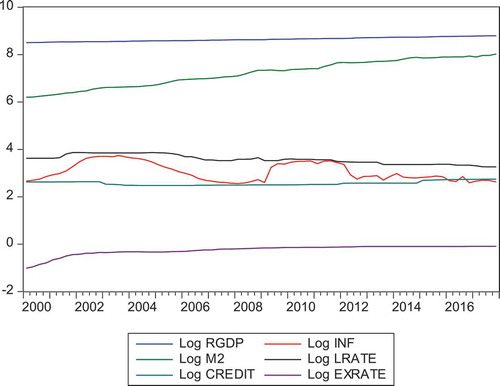
The graph reveals that, as money supply and inflation increase, real GDP and lending rate also decreases and exchange rate increases: an increase in money supply by Bank of Ghana has helped to increase inflation which has affected exchange rate to increase. From the graph, the rate of increasing real GDP is very low as compared to the rate of increasing money supply; due to this, there is less investment, innovations, exports but more imports in Ghana. This has affected the lending rate to decreased slightly from 37.50% in January, 2000 to 31.33%. The high lending rate (31.33%) in Ghana and the low output (GDP) have affected the exchange rate to increase; due to this, there is less investment, innovation, exports but more imports. This has caused the exchange rate to appreciate (increase) and that is why inflation in Ghana is too high.
Figure 2. Graphs of Differenced Series of Variables in the Ghanaian Money Market
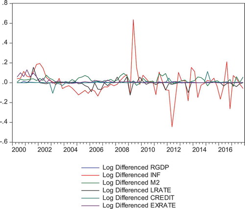
On differencing the series once, they tended to fluctuate around their mean suggesting that they became stationary. That is, they tended to exhibit similar behavior on differencing. This is depicted in Figure . According to Stigler and Sherwin (1985), unrelated variables might have high correlation coefficient using the levels but on differencing, they exhibited low correlation coefficient. However, two related nonstationary variables tended to have high correlation coefficient both in levels and first differences. The real GDP, inflation, the exchange rates, the lending rate and broad money supply exhibited similar movement in first differences as shown in Figure above.
3.3. Stationarity test
The time series property of each variable is examined using the Philip-Perron test for the unit root. Once the variables are stationary, the results generated would not be spurious. The results are found in .
From Table 2, when each variable is examined through level, the calculated PP statistics reject the null hypothesis since the P value is more than 5%; that is, the p value for PP—Fisher Chi-square is 0.9992. This means that the variables in the VAR model is not stationary. The variables were differenced to inquire if stationarity can be achieved. The results are presented ().
From Table 3, when each variable is examined through first difference, the calculated PP statistics accepted the null hypothesis that there is unit root at 5% significant levels when compared with the relative critical values; that is, P value for PP—Fisher Chi-square is 0.0000. This means that the variables in the VAR model are stationary. The null hypothesis of the presence of a unit root is rejected since the p values for the various macroeconomic variables are less than 5% at first difference. This paves the way for the study to estimate the VAR model.
3.4. Stability and reliability of the optimal lag VAR model
It is essential to determine the optimal lag length of the model before estimating a VAR model. The AIC was used in selecting the number of lags and it proposed three lags. In the regressions of the base and the extended models, three (3) lags were used as maximum number of lags due to the limited number of observations. The results for checking the optimal lag lengths for the VAR model are presented in below.
The inverse roots of the AR characteristics polynomials that lie within the unit circle indicated that there was no problem in terms of stability of three-lag VAR model for the base model and stability of lag-one for RGDP and INF models. Moreover, the reliability of the model whose lag length was determined to be three (3) was also confirmed on the basis of the 0.05 significance level found in three diagnostic tests: namely, the Breusch-Godfrey (Serial Correlation), L.M. White (Heteroscedasticity) and Multivariate normality of the VAR Residuals for all the models (see Appendix 2).
3.5. Analysis of the base VAR models
The original VAR regression results are provided in the Appendix. From the VAR regression results, the granger causality tests, impulse response functions, and forecast error variance decompositions estimates are derived and presented accordingly by beginning with the base VAR model. Vector autoregression is used extensively in econometric analysis because they are easy to specify and estimate; however, if the process is stationary or involves nonstationary cointegrated variables, it is usually difficult to interpret the VAR coefficients directly (Lütkepohl & Saikkonen, 1997). Therefore, granger causality test, impulse response analysis and forecast error variance decomposition are the alternative approaches proposed which help in understanding the relation among variables of the VAR system. According to STOCK and WATSON (2001), granger-causality tests, impulse responses and forecast error variance decompositions are more informative to understanding the relationships among the variables than the VAR regression coefficients or R2 statistics.
3.6. Granger causality/block exogeneity test: the base mode
The granger causality test is taken for the base model to find out if lagged values of broad money supply, lending rate, credit to private sector ratio and exchange rate contain any information that could predict real output, and inflation. The test result is accessible in
The Granger causality test results in show that real GDP granger cause exchange rate at the 5% significance level. Money supply, lending rate and inflation do not granger cause exchange rate. The implication is that, past values of money supply, lending rate and inflation cannot be used to forecast the present value of exchange rate.
Real Gross Domestic Product (RGDP) has a significant effect on exchange rate. The implication is that; real GDP can be used to forecast the present value of exchange rate. However, money supply has a significant effect on real gross domestic product (RGDP). The implication is that past values of money supply can be used to forecast the present value of real gross domestic product (RGDP). Monetary theory suggests that an increase in the money supply leads to an increase in the price level and a potential increase in real GDP.
3.7. Impulse responses for the base model for exchange rate
To buttress the information adduced in the granger causality test, a confirmation and direction was sought by looking at the impulse responses for the overall effect of money supply, lending rate, real GDP and inflation rate on exchange rate. The results are shown in Figure . The dotted lines representing ±2 standard error confidence intervals and on horizons given 10-year periods.
Figure 3. Responses of Real GDP to Exchange Rate
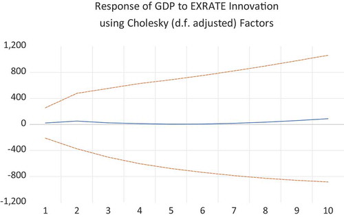
A positive shock to real GDP leads to a negative response of exchange rate which is persistent and thus last throughout the tenth year as shown in Figure . This confirms the result obtained in the granger causality test. Theoretically Keynes had explained that when money supply increases interest rate falls, investment increases and real GDP increases. Empirical studies such as Dilmaghanti and Tehranchian (2015) and Muchiri (2017) confirm a negative relationship between GDP and Exchange rate. The study accepts the alternative hypothesis that real GDP has a significant impact on exchange rate. The combined Wald Test of the significance of real GDP having effect on exchange rate has been confirmed at 5% level of significance with a p value of 0.0000. [See Appendix 3.]
Figure 4. Responses of Inflation to Exchange Rate
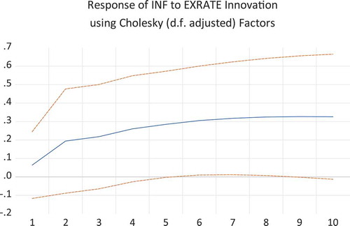
A one standard deviation inflation shock on exchange rate results in a positive impact that is transitory and last throughout for ten years.
This inconsistency vis-à-vis the response of inflation to exchange rate, as explained above, could be attributed to such other factors as instability in the nominal interest rate. This also confirm the result from granger causality test. Empirical studies such as Dilmaghanti and Tehranchian (2015) and Nduri (2013) confirm a positive relationship between inflation and Exchange rate (Figure ).
Figure 5. Responses of Money Supply to Exchange Rate
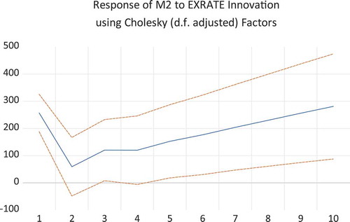
A one standard deviation money supply shock on exchange rate results in a positive impact that is transitory and last throughout for ten years. Empirical studies such as Eichengreen (2004) and Muchiri (2017) confirm a positive relationship between money supply and Exchange rate (Figure ).
Figure 6. Responses of Lending Rate to Exchange Rate
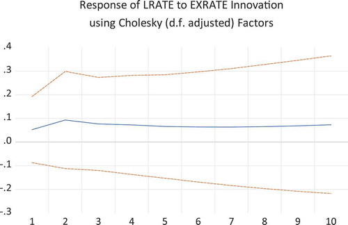
A one standard deviation lending rate shock on exchange rate results in a negative impact that is transitory and last throughout for ten years. Empirical studies such as Nduri (2013) and Muchiri (2017) confirm a negative relationship between lending rate and Exchange rate.
3.8. Forecast error variance decomposition: the base model
The Cholesky Forecast Error Variance Decomposition (FEVD) helps determine a shock of fluctuations in a variable caused by shocks on other variables. The variance decomposition is calculated for the third, sixth and the tenth years. The outcome is shown in Table 7.
The variance decomposition demonstrates that inflation rate shocks are a very important source of fluctuations in exchange rate, accounting for 10.70120% % shocks in exchange rate in the longer horizon of ten years, followed by lending rate accounting for 1.841566% shocks in exchange rate in the longer horizon of ten years. Real GDP is the next source of fluctuations in exchange rate, accounting for 1.019731% shocks in exchange rate in the longer horizon of ten years. Money supply is the last source of fluctuations in exchange rate, accounting for 0.548307% shocks in exchange rate in the longer horizon of ten years.
3.9. Hypothesis test result of the VAR base model for Ghana
The hypothesis tested was that macroeconomic variables impact exchange rate in Ghana. The joint Wald Test of the significance of the previous values of real GDP, inflation and money supply having effect on exchange rate have been confirmed at 5% level of significance of real GDP, inflation and money supply with a p value of 0.0000% on exchange rate, but the past values of lending rate could not help predict the current level of exchange rate with a p value of 0.3164%.
4. Conclusion
The results indicate that GDP in Ghana is low and as a result, has caused the exchange rate in Ghana to increase. To this effect, Ghanaian policymakers need to implement a set of policies geared towards improving investment efficiency and bolstering consumption.
The Bank of Ghana should loosen its credit ceilings to support credit expansion for economic growth as done in other countries. This will result in a more rapid expansion in credit which can lead to somewhat more rapid real GDP growth.
The interest rate (lending rate) should be more liberalized so that it can reflect the supply and demand of the money market better. Interest rate should be controlled in a more responsive way to catch up with inflation rate as well as to mitigate bad effects on the economy.
The Bank of Ghana should continue enticing reputable foreign banks, especially Asia Banks, into the Ghanaian market with a view to importing banking expertise, increasing competition and efficiency of bank operations and lowering interest rate spreads among commercial banks. In the medium term, this is capable of enforcing the deepening of financial intermediation which will be crucial to strengthening the interest rate and bank lending channel.
4.1. Practical limitations of the study and suggestions for future research
In undertaking a study of this kind, a number of caveats need to be taken into account while interpreting the results. The first weakness has to do with the VAR technique employed in this study. Most often than not, econometric techniques employed in analyzing level relationships among variables may be replete with limitations for policy recommendations. The results from these techniques may be divergent from the many theoretical underpinnings of level relationships. The implication is that their interpretations may be misleading. Moreover, even if the results are in tangency with theoretical foundations, the fact that different econometric software report different critical values depending on the sample size employed may lead to the failure of rejection of a null hypothesis, even if they are untrue.
These limitations offer important guidelines and suggestions for future research purposes. For example, further studies could be undertaken on a longer horizon time scale if supportive data is available. In this case more lags can be applied to have a conspicuous picture of the response of macroeconomic variables to exchange rate shocks.
Again, the study was devoid of any exogenous variable and as such other exogenous variables such as FDI, unproductive government spending and balance of payment may be considered in the model.
Moreover, a different shock variable (M2 was used in this study) such as M2+ could be used as a measure of exchange rate shock and as part of a different variable mix in addition to the government consumption.
Additional information
Funding
Notes on contributors
Samuel Antwi
Dr Samuel Antwi is currently a senior lecturer and also the Vice Dean of the School of Graduate Studies at University of Professional Studies, Accra. He is the former Director of Research and former Dean of the School of Graduate Studies of the Koforidua Technical University.
He obtained his Bachelor of Business Administration from 1996 to 2000 from University of Ghana and Master of Business administration (Accounting Option) from 2001 to 2003 from University of Ghana. He had a PhD from Jiangsu University in China. His research interests cover the corporate failure predictions, performance measurement, macroeconomic variables and risk management.
The study major contribution is that exchange rate stability achieved through stable macroeconomic variables gives credibility to the economy of a country to local and foreign trade partners and fluctuations in exchange rates may have a direct influence on trade balance, price stability and financial stability.
References
- Adusie, M., & Gyampong, E. Y. (2007). The impact of macroeconomic variables on exchange rate volatility in Ghana: The partial least squares structural equation modelling approach. Journal of Research on International Business and Finance, 42, 1428–19.
- Alagidede, P., & Muazu, I. (2016). An analysis on the causes of real exchange rate volatility and its effect on economic growth in Ghana. International Growth Center.
- Antwi, S., Boadi, E. K., & Okoranteng, E. O. (2014). Influential factors of exchange rate behaviour in Ghana. A cointegration analysis. International Journal of Economics and Finance, 6(2), 161–173.
- Appleyard, D. R., Field, J., Jr., & Cobb, S. L. (2006). International Economics. McGraww-Hill.
- Bawumia, M., & Abradu-Otoo, P. (2003). The relationship between monetary growth, exchange rates and inflation in Ghana: An error correction analysis. Open Journal of Social Sciences, 7, 3.
- Bawumia, M., Abradu-Otoo, P., & Amoah, B. (2003). An investigation of the transmission mechanism of monetary policy in Ghana: A structural vector error correction analysis. Working Paper. WP/BoG 2003/02. Bank of Ghana.
- Dilmaghanti, A. K., & Tehranchian, A. M. (2015). The impact of monetary policies on the exchange rate: A GMM approach. Iran Economics Review, 19(2), 177–191.
- Eichengreen, B. (2004). Monetary and exchange rate policy in Korea: Assessments and policy issues. Paper prepared for a symposium at the Bank of Korea, Seoul.
- Ghanaian chronicle. (2017). Bank of Ghana: Monetary policy summary. https://www.modernghana.com/news/755606/bank-of-ghana-monetary-policy-summary.html
- Laryea, M. N. (2016). Exchange rates and economic recovery program (ERP): A monetary approach to Ghana’s exchange rate 1972-2013 [unpublished master’s thesis]. Department of Business Administration, Asheshi University College, Ghana.
- Lütkepohl, H., & Saikkonen, P. (1997). Impulse response analysis in infinite order cointegrated vector autoregressive processes. Journal of Econometrics, 81(1), 127–157. https://doi.org/10.1016/S0304-4076(97)00037-7
- MacKinnon, J. G. (1996). Numerical distribution functions for unit root and cointegration tests. Journal of Applied Econometrics, 11(6), 601–618. https://doi.org/10.1002/(SICI)1099-1255(199611)11:6<601::AID-JAE417>3.0.CO;2-T
- Mankiw, N. G. (2006). Macroeconomics (5th ed.). Thompson Southern-Western Publishers.
- Muchiri, M. (2017). Effect of inflation and interest rates on foreign exchange rates in Kenya [Masters Dissertation]. https://www.coursehero.com/file/32524038/Muchiri-Effect-Of-Inflation-And-Interest-Rates-On-Foreign-Exchange-Rates-In-Kenyapdf/
- Nduri, O. M. (2013). The effect of interest rate and inflation rate on exchange rates in Kenya [Masters Dissertation].http://erepository.uonbi.ac.ke/bitstream/handle/11295/63359/Okoth_Inflation%20rate.pdf?sequence=3&isAllowed=y
- Owusu-Afriyie, E., & Mumuni, Z. (2004). The determinants of Cedi/Dollar rate of exchange in Ghana: A monetary approach Working paper, WP/BOG-2004/06, 1–23
- Ozkan, I., & Erden, L. (2015). Time-varying nature and macroeconomic determinants of exchange rate pass-through. International Review of Economics and Finance, 38(1), 56–66. https://doi.org/10.1016/j.iref.2015.01.007
- Sims, C. (1980). Macroeconomics and reality. Econometrica, 48(1), 1–49. https://doi.org/10.2307/1912017
- Stigler, G. J., & Sherwin, R. A. (1985). The extent of the market. The Journal of Law and Economics, 28(3), 555–585.
- STOCK, J. H., & WATSON, M. W. (2001). Vector auto regressions. Journal of Economic Perspectives, 15(4), 101–116. https://doi.org/10.1257/jep.15.4.101
- Tomiwa, S. (2018). The impact of real interest rate on real exchange rate: Empirical evidence from Japan. 2018 Awards for Excellence in Student Research and Creative Activity, 5.
Appendices
Appendix 1: OPTIMAL LAG LENGTH CHECKS FOR THE VAR MODEL
Table A1. Optimal lag length checks for the Basic VAR Model for Ghana
Appendix 2.
AUTOCORRELATION, HETEROSKEDASTICITY, NORMALITY AND AR ROOTS TESTS
Table A2. VAR Residual correlation LM TEST
Table A3. VAR Residual Portmanteau Test for Autocorrelations
HETEROSKEDASTICITY TESTS
Table A4. VAR Residual Heteroskedasticity Test for the Base VAR Model
VAR NORMALITY TESTS
Table A5. VAR Residual Normality Test for Skewness
Table A6. VAR Residual Normality Test for Kurtosis
Table A7. VAR Residual Normality Test for Jarque-Bera
ROOTS OF CHARACTERISTIC POLYNOMIAL
Appendix 3.
Wald Test on Significance of Var Coefficients for Ghana
Table A8. VAR Lag Exclusion Wald Tests Chi-squared test statistics for lag exclusion: Numbers in () are p values
Appendix 4.
VAR MODEL REGRESSION RESULTS
Table A9. Regression Result for the Base VAR Model for Ghana Standard Errors in () and t-Statistics []