A SAM framework for general equilibrium modeling and economic policy analysis

Abstract

Social accounting matrix (SAM) is the linkage bridge between economic data and policy analysis in the general equilibrium models. While the empirical SAM is built upon economic data from the system of national accounts, the theoretical SAM is built upon the relation between economic actors in the economy. This paper proposes the SAM framework for the data linkage between the empirical SAM and the theoretical SAM, in which the SAM structure is defined with endogenous and exogenous blocks. The endogenous activities involve the production, income generation, and expenditures in the economy. The exogenous activities involve income redistribution, asset transfer, and capital accumulation of the economy. From the SAM framework, the general equilibrium model with the objective function of GDP, the equilibrium price system, and the constraints of macro balances are developed for experimental simulation and economic policy analysis. The paper contributes to the SAM framework that provides fundamental insights into economic data, SAM structure, and general equilibrium model for economic policy analysis.

Keywords:

• SAM
• GDP
• general equilibrium
• economic data
• policy analysis

PUBLIC INTEREST STATEMENT

The social Accounting Matrix (SAM) always takes a crucial role in general equilibrium modeling and economic policy analysis. The big challenge is how to use economic data from the system of national accounts (SNA) for general equilibrium modeling, and experimental results from the general equilibrium model for economic policy analysis. This paper proposes the SAM framework with the data linkage between the empirical SAM and the theoretical SAM, and then uses the SAM framework for general equilibrium modeling. Since the paper integrates economic data from SNA and macro policies into the general equilibrium model, it provides an effective tool for economic policy analysis.

1. Introduction

The social accounting matrix (SAM) always plays a crucial role in general equilibrium modeling and economic policy analysis. SAM is a comprehensive database on the production activities of the economy that contain information on interactive relationship and resource transfer among economic actors in the economy for a certain period of time (Pauw, 2003). Therefore, the social accounting matrix (SAM) has become an essential economic database for strategic economic researchers and economic policymakers. According to King (1985), SAM has two main goals: The first goal of SAM is data organization, in which the accounts in SAM represent economic actors related to economic transactions. These transactions are recorded in SAM’s relevant accounts. Therefore, SAM forms a complete database of all transactions among economic actors within a certain period of time that provides a “comprehensive picture” of the structure of an economy. The second goal of SAM is not only to provide input data but also to update experimental results from economic models, especially for general equilibrium models. The structure and data of SAM allow planners to study macroeconomic policies and the operations of the economy over time.

There are two popular approaches for the economic accounting system: the System of National Accounts (SNA) was developed by the United Nations (United Nations, 1968), and the National Income and Product Accounts (NIPAs) was developed by the United States (McCulla & Mead, 2007). The difference in the SAM approach depends on the economic accounting system. Pyatt (1985, 1988) constructs SAM upon the NIPAs framework that presents the relation between economic actors. Although the theoretical SAM approach has well support in general equilibrium modeling for economic policy analysis, but most countries use the SNA framework instead of the NIPAs framework. Santos (2010, 2011) constructs SAM upon the SNA framework representing national accounts and aggregate economic indicators. However, the empirical SAM does not support input data directly for general equilibrium models. The problem is how to construct a SAM framework that integrates the theoretical SAM and the empirical SAM. To deal with this problem, this paper defines the SAM structure with two blocks of endogenous activities and exogenous activities. While the endogenous activities drive on the GDP of the economy, the exogenous activities affect the well-being and the GDP in the future. The SAM framework is built upon data linkage between the empirical SAM and the theoretical SAM. The empirical SAM provides economic data for the theoretical SAM in general equilibrium modeling, and then the simulation results are updated into the empirical SAM for economic policy analysis.

From the SAM framework, the basic general equilibrium model is developed with the objective function of GDP, the equilibrium price system, and constraints of macro balances. The general equilibrium model uses the theoretical SAM data for the experimental simulations, and then the experimental results are updated into the empirical SAM for economic policy analysis. The paper is organized into four main sections. The next section proposes the SAM framework with the data linkage between the empirical SAM and the theoretical SAM. Section 3 develops a basic general equilibrium model under the SAM framework for economic policy analysis. The last section summarizes the main results and also suggests limitations for further researches.

2. Social Accounting Matrix

Stone (1961, 1962) is a pioneer proposing the presentation of national accounting not only in the account “T” but also in the form of social accounting matrix (SAM), in which SAM describes the diversity of economic activities with different statistical units for economic actors in the economy. SAM represents accounting data for fund flows in the circular flow diagram of the economy. The SAM structure is a square matrix in which each row and column is called an “account”. Each cell in the matrix represents a fund movement from a column account to a row account. The double entry rule requires the inflow to be equal to the outflow for each account in SAM. This also means that the total row must be equal to the total column for each account.

The starting point for the SAM framework is the definition of SAM structures of the theoretical SAM and the empirical SAM. The theoretical SAM is constructed upon the economy’s structure to study the relationship between economic actors in markets as shown in Figure 1. The basic structure of the economy shows how economic actors (households, enterprises, governments, and rest of the world) interact in markets (commodity markets, factor markets, and financial markets) under macro balances (investment-saving balance, government balance, and trade balance).

Figure 1. Circular flow diagram of the economy.

Source: Trinh (2019)

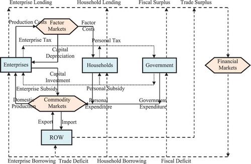
The circular flow diagram is a simplified representation of the structure of the economy. The underlying principle is that fund inflow into each market or institution is equal to fund outflow of that market or institution. The structure of the theoretical SAM describes the relation between economic actors as in Table 1. Therefore, the theoretical SAM supports general equilibrium models for economic policy planning (Pyatt, 1988).

Table 1. The structure of theoretical SAM

	Commodity C1	Factor C2	Households C3	Enterprises C4	Government C5	Financial C6	ROW C7	Total
Commod ity R1			Perso nal Expendi ture (C)	Capital Investment (I)	Government Expenditure (G)		Export (X)	Total Demand
Factor R2				Production Costs (KWK+ LWL)				Factor Demand
Households R3		Factor Costs (KWK + LWL)			Personal Subsidy (SbP)	Household Borrowing (Sc < 0)		Household Inflow
Enterprises R4	Domestic Production (GDP)				Enterprise Subsidy (SbF)	Enterprise Borrowing (П < 0)		Enterprise Inflow
Government R5			Personal Tax (TP)	Enterprise Tax (TF)		Fiscal Deficit (G > T)		Government Inflow
Financial R6			Household Lending (Sc>0)	Enterprise Lending (П > 0)	Fiscal Surplus (G < T)		Trade Surplus (X < N)	Financial Demand
ROW R7	Import (N)					Trade Deficit (X > N)		ROW Inflow
Total	Commodity Supply	Factor Supply	Household Outflow	Enterprise Outflow	Government Outflow	Financial Supply	ROW Outflow

Source: Trinh (2019)

The final commodities are supplied by domestic producers [R5-C1] and imported from the world (ROW) [R7-C1]. Total supply must be equal to total demand including personal spending [R1-C3], investment capital [R1-C4], government expenditure [R1-C5], and export [R1-C7]. The production factors are provided by households [R3-C2]. Total supply of production factors is equal to the total cost of production [R2-C4] of the enterprises. Financial supply comes from household saving [R6-C3] and enterprise profit [R6-C4]. Financial demand includes government borrowing [R5-C6] and the world borrowing (ROW) [R7-C6] for offsetting deficits, household borrowing [R3-C6], and enterprise borrowing [R4 -C6].

Households receive income from the provision of capital and labor [R3-C2], and use for their personal expenditure [R1-C3]. Households can deposit their saving on the financial market [R6-C3] or borrow their deficit from financial markets [R3-C6]. Enterprises pay for production costs [R2-C4], investment capital [R1-C4], and enterprise taxes [R5-C6]. Enterprises also receive revenue from domestic production [R4-C1]. Enterprises can send their profit on financial markets [R6-C4] or borrow money from financial markets [R4-C6]. The government collects taxes from households [R5-C3] and enterprises [R5-C4], and returns apart to personal subsidy [R3-C5] and enterprise subsidy [R4-C5]. The rest is for government expenditure [R1-C5]. The government either borrows for budget deficit [R5-C6] or sends a budget surplus on the financial market [R6-C5]. ROW pays for exports [R1-C7] and receives from import [R7-C1]. ROW sends trade surplus [R6-C7] to the financial market or borrows a loan to offset the trade deficit [R7-C6] from the financial market.

Meanwhile, the empirical SAM is constructed upon economic data of the system of national accounts (SNA). The empirical SAM structure represents aggregate economic indicators with the consistency of the entire system that allows economists to compare the economic activities of a country with other countries.

Figure 2 illustrates the relationship between national accounts in the economy that starts with the product, production, and factor accounts. The inflows of these accounts come from foreign countries (net exports), capital accounts (investment capital), current accounts (household and government consumption), and production accounts (demand of intermediate inputs). The income of these accounts is used to pay for domestic demand from production accounts as well as taxes and subsidies on product and production.

Figure 2. Fund flows between the accounts in the economy.

Source: Santos (2010)

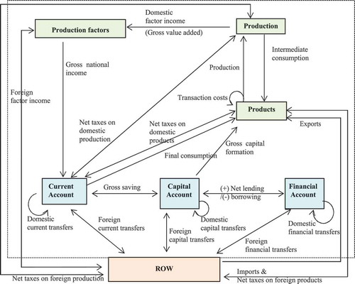
The production account adds the value of intermediate inputs into final commodities purchased by the product account. These fund flows are represented by payments for factor accounts and product accounts. Production taxes are paid to the government present in the current account.

Besides factor income is received from production accounts, transfers are received as additional income from the ROW account. Because the economic actors own production factors, income from factor accounts is paid to economic actors through the current account. Transfers between domestic economic actors show the movement of fund flows in the current account, capital account, and financial accounts. These transfers include tax payments from households and enterprises to the government, transfers between households, transfers from the government to households such as social security benefits, and all other transfers between economic actors. In addition, net foreign transfers influence the wealth of economic actors.

The portion of aggregate income that is not used for final consumption expenditure and current transfers to economic actors is gross saving. Government saving can be negative (budget deficit) or positive (budget surplus). The gross saving of economic actors from the current account is transferred to the capital account. The trade balance and foreign transfer will affect the total debt. Total saving and total debt will influence investment capital in the future. This represents a stream of transfers from the capital account to the product account.

Table 2 describes the transactions between national accounts that are aggregated into the cells of the empirical SAM. The aggregate economic indicators in the empirical SAM are summarized from SNA accounts as shown in Table 3.

Table 2. The structure of the empirical SAM

	Product C1	Production C2	Factor C3	Current C4	Capital C5	Financial C6	ROW C7	Total
Product R1	Transaction costs (TTM)	Intermediate consumption (IC)		Final consumption (FC)	Gross capital formation (GCF)		Exports (EX)	Aggregate Demand
Production R2	Gross output (GO)							Production Value
Factor R3		Gross value added (GAV)					Factor income from RW (CFPEX)	Factor Income
Current R4	Net taxes on products (NTP)	Net taxes on domestic production (NTADM)	Gross national income (GNI)	Domestic current transfers (CT)			Current transfers from RW (CTEX)	Current Inflow
Capital R5				Gross saving (GS)	Domestic capital transfers (KT)	Net borrowing/lending (NLB)	Capital transfers from RW (KTEX)	Capital Inflow
Financial R6						Domestic financial transfers (FT)	Financial transfers from RW (FTEX)	Financial Inflow
ROW R7	Imports (IM)	Net taxes on foreign production (NTAIM)	Factor income to RW (CFPIM)	Current transfers to RW (CTIM)	Capital transfers to RW (KTIM)	Financial transfers to RW (FTIM)		ROW Inflow
Total	Aggregate Supply	Production Cost	Factor Outcome	Current Outflow	Capital Outflow	Financial Outflow	ROW Outflow

Source: Adapted from Santos (2010)

Table 3. The aggregate economic indicators in the empirical SAM

SAM			Aggregate economic indicators
Row	Column	Description (valuation)	SNA Code	Description (valuation)
R2	C1	Production (basic prices)	P1	Gross output (basic prices)
R4	C1	Net taxes on products	D21-D31	Taxes on products minus subsidies on products
R7	C1	Imports (cif prices)	P7	Imports of goods and services (cif prices)
R1	C7	Exports (fob prices)	P6	Exports of goods and services (fob prices)
R1	C2	Intermediate consumption (purchasers’ prices)	P2	Intermediate consumption (purchasers’ prices)
R1	C4	Final consumption (purchasers’ prices)	P3	Final consumption (purchasers’ prices)
R1	C5	Investment capital	P5	Gross capital formation
R3	C2	Gross added value (factor costs)	D1 + B2g + B3g	Compensation of domestic factors
R4	C2	Net taxes on domestic production	D29- D39	Taxes on production minus Subsidies on production
R7	C2	Nets taxes on foreign production
R4	C3	Gross national income	B5g	Gross national income
R7	C3	Factor income to the RW(resources)	D1+ D4	Compensation of foreign factors
R3	C7	Factor income from the RW(uses)
R4	C4	Domestic current transfers institutions	D5+ D6+ D7 + D8	Current transfers
R7	C4	Current transfers to the RW (resources)
R4	C7	Current transfers from the RW (uses)
R5	C4	Gross saving	B8g	Gross saving
R5	C5	Domestic capital transfers	D9	Capital transfers
R5	C7	Capital transfers from the RW (uses)
R7	C5	Capital transfers to the RW (resources)
R5	C6	Net borrowing/lending (+lending/-borrowing)	B9	Net borrowing/lending (+lending/-borrowing)
R6	C6	Domestic financial transfers	F1→F8	Financial transfers
R7	C6	Financial transfers to the RW (resources)
R6	C7	Financial transfers from the RW (uses)

Source: Santos (2011) and Author’s study.

The aggregate economic indicators reflect all transactions of national accounts in SAM. Table 4 illustrates the relationship between the main aggregate economic indicators between the theoretical SAM and the empirical SAM.

Table 4. The aggregate economic indicators in SAM

Aggregate economic indicators	The theoretical SAM	The empirical SAM
Final consumption	C + G	FC
Investment capital	I	GCF
Exports	X	EX
Imports	N	IM
Gross domestic product	GDP	-
Net taxes and subsidies	T	NTP + NTA
Domestic factor income	K× WK + L× WL	-
Gross value added	-	GAV
Gross national income	-	GNI

Source: Author’s research.

For economic policy analysis, economic data from national accounts are aggregated into the empirical SAM structure. The illustrated data from the SNA 2008 is used for the empirical SAM as in Table 5.

Table 5. The statistical data for the empirical SAM

	Product C1	Production C2	Factor C3	Current C4	Capital C5	Financial C6	ROW C7	Total
Product R1		1883		1399	414		540	4236
Production R2	3604							3604
Factor R3		1663					44	1707
Current R4	133	62	1669	1168			17	3049
Capital R5				427	61	−10	1	479
Financial R6						379	47	426
ROW R7	499	−4	38	55	4	57		649
Total	4236	3604	1707	3049	479	426	649

Source: Author’s calculations from SNA 2008 (United Nations., European Commission., International Monetary Fund., Organisation for Economic Co-operation and Development. and World Bank, 2009).

Economic policy analysis concerns policy impacts on economic actors, industrial structure changes, household income, and macro balances. This requires researchers and economists to collect statistical data and investigate economic actors. The theoretical SAM allows not only the estimation of aggregate economic indicators but also the ability to analyze the impact of economic policies on the national economy.

However, the major limitation of the theoretical SAM relates to statistical techniques and investigation ability to economic actors. Therefore, the SAM structure is divided into two blocks of endogenous activities and exogenous activities. The endogenous block involves accounts of product and production in the SAM that will directly affect gross domestic product (GDP). Meanwhile, the theoretical SAM and the empirical SAM have different accounts in the exogenous block. While national accounts of households, enterprises, government, financial, ROW are constructed in the theoretical SAM, national accounts of factor, current, capital, financial, ROW are constructed in the empirical SAM. The endogenous data of the theoretical SAM are estimated from the endogenous data of the empirical SAM (Table 5) and SNA accounts based on the relationship in Table 4. From the double-entry rule, the exogenous data of the theoretical SAM are generated from the calibration process under given assumptions and current policies of the economy. The calibration process will estimate elasticities of the price system, initial equilibrium status of factor and commodity markets.

From the initial equilibrium condition and macro-policy setting, the general equilibrium model provides the experimental results for the theoretical SAM as in Table 6. Moreover, the experimental results present the GDP structure (under the expenditure approach and the income approach) and macro balances (investment-saving balance, government balance, trade balance).

Table 6. The experimental data of the theoretical SAM

	Commodity C1	Factor C2	Households C3	Enterprises C4	Government C5	Financial C6	ROW C7	Total
Commodity R1			1047	414	352		540	2353
Factor R2				752				752
Households R3		752				295		1047
Enterprises R4	1854							1854
Government R5				191		161		352
Financial R6				497				497
ROW R7	499					41		540
Total	2353	752	1047	1854	352	497	540

Source: Author’s calculations from SNA 2008 (United Nations., European Commission., International Monetary Fund., Organisation for Economic Co-operation and Development. and World Bank, 2009).

The gross domestic product is calculated as follows:

• The expenditure approach: GDP = C + G + I + X—N = 1854

• The income approach: GDP = K× W_K + L× W_L + П + T + I = 1854

The macro balances are determined as follows:

• The investment-saving balance: П + (C—K× W_K + L× W_L) = 202

• The government balance: T—G = −161

• The trade balance: X—N = 41

3. General Equilibrium Model

The general equilibrium mechanism is based on the general equilibrium theory (Walras, 1874), and the equilibrium existence of a general equilibrium model with some assumptions of the economy (Arrow & Debreu, 1954). On the theoretical basis, economists develop a general equilibrium model through mathematical approaches with the equilibrium equation system to maximize consumer benefits and enterprise profits (Hosoe et al., 2010; Lofgren et al., 2002; Sue Wing, 2004). The previous general equilibrium models define the objective functions of production and consumption under the underlying assumptions. In fact, these equilibrium equations and questionable assumptions are criticized on the price system for the ideal competitive economy. To eliminate drawbacks of the equilibrium equation approach, the general equilibrium programming model develops with the objective function of GDP, equilibrium price system, and constraints of macro balances.

The programming approach allows economists to conduct economic policies (economic shocks) on the GDP and macro balances in the real-world economy. Economic actors allocate resources towards maximizing the GDP or economic welfare under constraints of market equilibrium and macro balances. Whenever having the changes in production factors (capital and labor) will affect to production system of the economy. The price of input factors is changed upon the changes in input quantities, and the substitution effects through the values of price elasticity of factor demand and elasticity of factor substitution as follows:

(1) $W_{Kj}=W_{K0j}\times \left(1+\frac{\mathrm{\%}\mathrm{\Delta }{K}_j}{E_{DKj}^{WKj}}+\frac{\mathrm{\%}\mathrm{\Delta }{L}_j}{E_{DLj}^{WKj}}\right)$(1)

(2) $W_{Lj}=W_{L0j}\times \left(1+\frac{\mathrm{\%}\mathrm{\Delta }{K}_j}{E_{DKj}^{WLj}}+\frac{\mathrm{\%}\mathrm{\Delta }{L}_j}{E_{DLj}^{WLj}}\right)$(2)

where j is the index of sectors. W_K0, W_L0 are initial equilibrium prices of capital and labor, W_K, W_L are new equilibrium price of capital and labor, respectively. $\mathrm{\%}\mathrm{\Delta }K$, $\mathrm{\%}\mathrm{\Delta }L$ are percentage changes in capital and labor. $E_{DK}^{WK}$, $E_{DL}^{WL}$ are price elasticities of demand for capital and labor. $E_{DK}^{WL}$, $E_{DL}^{WK}$ are cross elasticities of demand between capital and labor.

The changes in production quantities and factor income will affect the price of final commodities. The interaction of markets is reflected through these values of elasticities that play an essential role in the price system. The price of final commodities is determined as the following formula:

(3) $p_j=\left(a_j+\frac{b_j}{1+E_{Dj}^I\times \mathrm{\%}\mathrm{\Delta }I}\times Q_{0j}\right)\times \left(1+\sum _{i=1}^m\frac{\mathrm{\%}\mathrm{\Delta }{Q}_i}{E_{Di}^{Pj}}\right)$(3)

(4) $a_j=p_{0j}-b_j\times Q_{0j}$(4)

(5) $b_j=\frac{1}{E_{Dj}^{Pj}}\times \frac{p_{0j}}{Q_{0j}}$(5)

where j index of sectors. Q₀ and p₀ are quantity demanded and price of initial equilibrium, respectively. p is the new equilibrium price. $\mathrm{\%}\mathrm{\Delta }Q$ and $\mathrm{\%}\mathrm{\Delta }I$ are percentage change in quantity demanded and Income, respectively. $E_{Dj}^{Pj}$ is the price elasticity of demand for the final commodity j. $E_{Dj}^I$ is income elasticity of demand for the final commodity j.

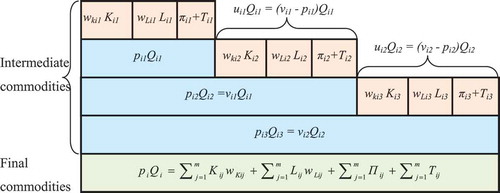
However, the price systems adjust resource allocation based on the objective function and market equilibrium conditions in the general equilibrium model. The optimal resource allocation with the objective function of GDP will maximize the production value under constraints of macro balances in the economy. Therefore, the GDP is an important measurement in resource allocation and economic policy analysis. Figure 3 illustrates the value-added method to measure the production value$\left(p_{ij}{Q}_{ij}\right)$ of sector i through the exchange processes between firms and customers.

The gross domestic product (GDP) of the economy including n industries is measured as follows:

(6) $GDP=\sum _{i=1}^n{p}_i\times Q_i+\sum _{i=1}^n{I}_i$(6)

(7) $GDP=\sum _{i=1}^n{K}_i\times w_{K_i}+\sum _{i=1}^n{L}_i\times w_{L_i}+\sum _{i=1}^n{\mathrm{\Pi }}_i+\sum _{i=1}^n{T}_i+\sum _{i=1}^n{I}_i$(7)

Figure 3. The approach for GDP measurement of sector i.

Source: Trinh (2017), Trinh (2018)

The general equilibrium model is developed upon institutions (households, enterprises, governments, and the rest of the world), markets (product market, factor market, financial market), and macro balances (investment-saving balance, government balance, trade balance). By changing economic policies (or economic shocks), market equilibrium and macro balances will be reestablished for the economy. The general equilibrium programming model is developed with the following main assumptions:

1. Households (customers) consume commodities (products or services) with the same preference and consumption parameters.

2. Enterprises (firms) provide m commodities (products or services) with the same technology and production parameters.

3. The economy has m industries (sectors), each sector produces a commodity (product or service).

4. Market equilibrium based on the price system (factors and products) is adjusted by the initial equilibrium price and the elasticities of supply and demand.

5. Rates of export price and domestic price (R_EX), taxes and subsidies (T), government expenditure (G), capital investment (I), are assumed in the models.

6. Macro balances are constrained upon target sector structure and macro policies relating to investment-saving, export-import, and government expenditure.

The basic general equilibrium programming model has the objective function of the GDP maximizing and constraints of market equilibrium and macro balances.

The general equilibrium programming model:

(8) $MaxGDP=\sum _{j=1}^{m}GD{P}_j$(8)

Subject to

(9) $W_{Kj}=W_{K0j}\times \left(1+\frac{\mathrm{\%}\mathrm{\Delta }{K}_j}{E_{DKj}^{WKj}}+\frac{\mathrm{\%}\mathrm{\Delta }{L}_j}{E_{DLj}^{WKj}}\right)\hspace{0.17em}\mathrm{\forall }j=\mathrm{1..}m$(9)

(10) $W_{Lj}=W_{L0j}\times \left(1+\frac{\mathrm{\%}\mathrm{\Delta }{K}_j}{E_{DKj}^{WLj}}+\frac{\mathrm{\%}\mathrm{\Delta }{L}_j}{E_{DLj}^{WLj}}\right)\hspace{0.17em}\mathrm{\forall }j=\mathrm{1..}m$(10)

(11) $Q_j^{\hspace{0.17em}}=A_j^{\hspace{0.17em}}\times K_j^{{\alpha }_j}\times L_j^{{\beta }_j}\hspace{0.17em}\mathrm{\forall }j=\mathrm{1..}m$(11)

(12) $p_j=\left(a_j+\frac{b_j}{1+E_{Dj}^I\times \mathrm{\%}\mathrm{\Delta }I}\times Q_{0j}\right)\times \left(1+\sum _{i=1}^m\frac{\mathrm{\%}\mathrm{\Delta }{Q}_i}{E_{Di}^{Pj}}\right)\hspace{0.17em}\mathrm{\forall }j=\mathrm{1..}m$(12)

(13) $a_j=p_{0j}-b_j\times Q_{0j};b_j=\frac{1}{E_{Dj}^{Pj}}\times \frac{p_{0j}}{Q_{0j}}\hspace{0.17em}\mathrm{\forall }j=\mathrm{1..}m$(13)

(14) $Q_j^{\hspace{0.17em}}=Q_{Cj}^{\hspace{0.17em}}+Q_{Gj}^{\hspace{0.17em}}+Q_{NXj}^{\hspace{0.17em}}\hspace{0.17em}\mathrm{\forall }j=\mathrm{1..}m$(14)

(15) $GD{P}_j=p_j\times \left(Q_{Cj}^{\hspace{0.17em}}+Q_{Gj}^{\hspace{0.17em}}+Q_{NXj}^{\hspace{0.17em}}\times R_{EXj}\right)+I_j\hspace{0.17em}\mathrm{\forall }j=\mathrm{1..}m$(15)

(16) $T_j=T_0\times GD{P}_j;I_j=I_0\times GD{P}_j\hspace{0.17em}\mathrm{\forall }j=\mathrm{1..}m$(16)

(17) $GD{P}_j=X_j\times \mathrm{G}\mathrm{D}\mathrm{P}\mathrm{\forall }j=\mathrm{1..}m$(17)

(18) $\sum _{j=1}^m{p}_j\times Q_{Gj}-\sum _{j=1}^m{T}_j\le A\mathrm{\%}\times GDP$(18)

(19) $\sum _{j=1}^m{p}_j\times Q_{NXj}\times R_{EXj}\le B\mathrm{\%}\times GDP$(19)

(20) $\sum _{j=1}^m{p}_j\times Q_{Gj}+\sum _{j=1}^m{P}_j\times Q_{NXj}\times R_{EXj}-\sum _{j=1}^m{T}_j\ge C\mathrm{\%}\times GDP$(20)

$\mathrm{\forall }{K}_j^{\hspace{0.17em}},L_j^{\hspace{0.17em}},w_{Kj},w_{Lj},p_j,Q_j,Q_{Cj},Q_{Gj},Q_{XNj},T_j,I_j\mathrm{\forall }j=\mathrm{1..}m$

Notations:

Indices:

i, j: indices of sectors (i, j = 1..m)

System parameters:

$A_j^{\hspace{0.17em}}$: Total factor productivity of sector j

${\alpha }_j^{\hspace{0.17em}}$: Output elasticity of capital of sector j

${\beta }_j^{\hspace{0.17em}}$: Output elasticity of labor of sector j

$K_{0j}^{\hspace{0.17em}}$: Initial equilibrium quantity of capital of sector j

$L_{0j}^{\hspace{0.17em}}$: Initial equilibrium quantity of labor of sector j

$w_{K0j}^{\hspace{0.17em}}$: Initial equilibrium price of capital of sector j

$w_{L0j}^{\hspace{0.17em}}$: Initial equilibrium price of labor of sector j

$p_{0j}$: Initial equilibrium price of final commodity of sector j

$Q_{0j}^{\hspace{0.17em}}$: Initial equilibrium quantity of final commodity of sector j

Policy parameters:

$X_j^{\hspace{0.17em}}$: Target GDP of sector j

$R_{EXj}$: Ratio of export price and domestic price

$T_0$: Ratio of tax and subsidy on GDP of sector j

$I_0$: Ratio of investment capital on GDP of sector j

$A\mathrm{\%}$: Ratio of government balance on GDP of the economy

$B\mathrm{\%}$: Ratio of trade balance on GDP of the economy

$C\mathrm{\%}$: Ratio of investment-saving balance on GDP of the economy

Decision variables:

$K_j^{\hspace{0.17em}}$: Quantity of capital of sector j

$L_j^{\hspace{0.17em}}$: Quantity of labor of sector j

$w_{Kj}^{\hspace{0.17em}}$: Unit cost of capital of sector j

$w_{Lj}^{\hspace{0.17em}}$: Unit cost of labor of sector j

$p_j^{\hspace{0.17em}}$: Price of final commodity of sector j

$Q_j^{\hspace{0.17em}}$: Quantity of final commodity of sector j

$Q_{Cj}^{\hspace{0.17em}}$: Quantity of personal consumption of sector j

$Q_{Gj}^{\hspace{0.17em}}$: Quantity of government consumption of sector j

$Q_{NXj}^{\hspace{0.17em}}$: Quantity of net export of sector j

$T_j^{\hspace{0.17em}}$: Net tax and subsidy of sector j

$I_j^{\hspace{0.17em}}$: Net investment capital of sector j

Experimental simulations are carried out on the hypothetical economy with m sectors from above basic general equilibrium model. Each sector j (j = 1..m) produces a commodity (product or service) with a total production output Q_j (j = 1..m) using the total capital (K_j) and the total labor (L_j). This model is based on the market equilibrium as in Constraint (14). The price system will adjust the price of input factors as in Constraints (9) and (10). The Cobb Douglas production function is expressed in Constraints (11), and the domestic product price is adjusted as in Constraints (12) and (13). Export prices are adjusted to the ratio of R_EXj (the ratio of export price and domestic price), which depends on the exchange rate, export price, and domestic price for sector j.

To analyse changes in economic policy, constraints of economic policy (16), (17), (18), (19) and (20) are added to the general equilibrium models. Constraints (15) and (17) measure GDP and establish a target GDP structure for each sector of the economy $\left(P_j\times Q_j=X_j\right)$ (j = 1..m), respectively. Constraints (18) set minimum government balance (government revenue from tax and subsidy $\left(\sum _{j=1}^m{T}_j\right)$ minus government expenditure)$\left(\sum _{j=1}^m{P}_j\times Q_{Gj}\right)$. Constraints (19) set maximum constraints for trade balance $\sum _{j=1}^m{P}_j\times Q_{NXj}\times E{X}_j$. Constraint (20) establishes a minimum constraint for investment-saving balance $\left(\sum _{j=1}^m{P}_j\times Q_{Gj}+\sum _{j=1}^m{P}_j\times Q_{NXj}\times E{X}_j^{\hspace{0.17em}}-\sum _{j=1}^m{T}_j\right)$, in which the investment-saving balance is equal to the subtraction of trade balance $\left(\sum _{j=1}^m{P}_j\times Q_{NXj}\times E{X}_j^{\hspace{0.17em}}\right)$ and government balance $\left(\sum _{j=1}^m{T}_j-\sum _{j=1}^m{P}_j\times Q_{Gj}\right)$.

Experimental simulation is undertaken with hypothetical settings of system parameter, market parameters, and policy parameters. The general equilibrium model will provide an optimal resource allocation solution to maximize the GDP of the economy. Since the structure of GDP represents household income, enterprise profit, and government tax income. Maximizing the GDP will allocate resources based on market equilibrium and value balance of economic actors. Since the GDP is not yet a good indicator of social welfare and macro stability, macro policies (18), (19), (20) will integrate into the general equilibrium model under the constraints of macro balances.

To conduct changes in economic policies, the experimental simulation assumes that the economy has three main sectors (agriculture, industry, services) (j = 3). The system parameters of the economy are given in Table 7.

Table 7. System parameters of the economy

Sectors	Symbol	Agriculture	Industry	Services
Total factor productivity	Aj	1	0.8	1.2
Output elasticity of capital	αj	0.6	0.5	0.7
Output elasticity of labor	βj	0.4	0.5	0.3
Initial equilibrium quantity of capital	K0j	30	15	45
Initial equilibrium quantity of labor	L0j	25	30	20
Initial equilibrium price of capital	wKj	6	5	7
Initial equilibrium price of labor	wLj	5	5	6
Initial equilibrium price of final commodity	pj	25	20	30
Initial equilibrium quantity of final commodity	Qj	27.89	16.97	42.34
Ratio of export price and domestic price	REXj	1	1.1	0.9
Current sector structure	%GDP	30%	35%	35%

Source: The hypothetical data for the experimental simulation.

The system parameter provides the sectors’ the production function parameters with the initial equilibrium status (price and quantity) of input factors and final commodities. Market parameters provide the elasticity values of input factor (Table 8) and final commodity (Table 9). These elasticity values are estimated upon changes in price and quantity of sectors from previous period data. The price system is based on the initial equilibrium price and elasticity of input factor to adjust and determine new equilibrium prices based on market equilibrium and macro balances.

Table 8. Elasticity of input factors

Elasticity of input factors	Capital demand DK	Labor demand DL
Capital price wK	$E_{DK}^{wK}=-0.5$	$E_{DL}^{wK}=2$
Labor price wL	$E_{DK}^{wL}=1$	$E_{DL}^{wL}=-1$

Source: The hypothetical data for the experimental simulation.

Table 9. Elasticity of final commodities

Elasticity of final commodities	Agriculture demand D1	Industry demand D2	Service demand D3
Agriculture price p1	$E_{D1}^{p1}=-1$	$E_{D2}^{p1}=0.5$	$E_{D2}^{p1}=1$
Industry price p2	$E_{D1}^{p2}=0.5$	$E_{D2}^{p2}=-0.8$	$E_{D3}^{p2}=-1.5$
Service price p3	$E_{D1}^{p3}=-0.5$	$E_{D2}^{p3}=-1$	$E_{D3}^{p3}=-1.2$
Income I	$E_{D1}^I=0$	$E_{D2}^I=-0.5$	$E_{D3}^I=0.5$

Source: The hypothetical data for the experimental simulation.

The macro balances are considered under constraints of tax, investment capital, target sector structure, government balance, trade balance, investment-saving balance as in Table 10.

Table 10. Policy parameters of the economy

Sectors	Symbol	Constraint	Value
Net taxes and subsidies	T0	=	13.26% ×(GDP—I)
Investment capital	I0	=	28.75%×(GDP—I)
Government balance	G—T	≤	10%×GDP
Trade balance	X—N	≤	20%×GDP
Investment-saving balance	G—T + X- N	≥	20%×GDP

Source: The hypothetical data for the experimental simulation.

To assess changes in sector structure and macro policies, policy parameters and macro constraints are set for experimental models as follows: Net taxes and subsidies (T) and net investment capital (I) changes along with GDP at a fixed rate (T₀ = 13.26% and I₀ = 28.75%) same rate as the current economy. The government deficit does not exceed 10% of GDP, the trade surplus does not exceed 20% of GDP, and the minimum rate of investment-saving is 20% of GDP. Depending on setting parameters of the macro policies, the experimental results will affect the GDP, resource allocation, market equilibrium, and macro-balance indicators.

There are three experimental models of the economy as follows:

Model 1: The current sector structure is 30% Agriculture, 35% Industry, and 35% Services.

Model 2: The optimal current economy with the same as the sector structure is 30% Agriculture, 35% Industry, and 35% Services.

Model 3: The transformation economy with the target sector structure is 30% Agriculture, 30% Industry, and 40% Services.

The experimental models of the economy are shown in Tables 11 and 12. Simulation results show that economic actors interact in markets. Table 11 shows the relationship between total output, expenditure and saving of economic actors. Table 12 shows GDP and macro balances. Investment-saving balance indicates the relationship between gross saving (household saving and enterprise profit) and net investment capital. Trade balance indicates the net value between exports and imports. Government balance indicates the relationship between government revenue (taxes and subsidies) and government expenditure. Policy analysis concerns on changes in macro balances and sector structure, and their impact on the GDP growth rate of the economy.

Table 11. Simulation results of the economy

Indicators	Formula	Model 1	Model 2	Model 3
Total output	$Q_j=Q_{Cj}+Q_{Gj}+Q_{NXj}$	58.22	80.98	82.86
Personal expenditure	$C=\sum _{j=1}^m{p}_j\times Q_{Cj}$	1047.00	1118.79	1178.34
Government expenditure	$G=\sum _{j=1}^m{p}_j\times Q_{Gj}$	352.00	479.52	505.04
Household saving	$S_C=\sum _{j=1}^m\left(K_j\times w_{Kj}+L_j\times w_{Lj}\right)-\sum _{j=1}^m{p}_j\times Q_{Cj}$	−295	−317.22	−390.96
Enterprise saving	$S_F=\sum _{j-1}^m{p}_j\times Q_j^{\hspace{0.17em}}-\sum _{j=1}^m{K}_j^{\hspace{0.17em}}\times W_{Kj}^{\hspace{0.17em}}-\sum _{j=1}^m{L}_j^{\hspace{0.17em}}\times W_{Lj}^{\hspace{0.17em}}-\sum _{j=1}^m{T}_j$	497.00	789.60	888.48
Government saving	$S_G=\sum _{j=1}^m{T}_j-\sum _{j=1}^m{p}_j\times Q_{Gj}$	−161	−236.19	−248.76
Total saving	$S=S_C+S_F+S_G$	41	236.19	248.76

Source: Trinh (2019) and Author’s research.

Table 12. The simulation results of GDP and macro balances

Indicators	Formula	Model 1	Model 2	Model 3
% Agriculture	$X_1$	30%	30%	30%
% Industry	$X_2$	35%	35%	30%
% Services	$X_3$	35%	35%	40%
GDP	$GDP$	1854.00	2361.92	2487.63
Government Balance	$\sum _{j=1}^m{p}_j\times Q_{Gj}-\sum _{j=1}^m{T}_j$	161	236.19	248.76
Trade Balance	$\times Q_{Gj}-\underset{j}{\overset{\hspace{0.17em}}{\sum _{j=1}^{m}T}}\sum _{j=1}^m{p}_j$	41	236.19	248.76
Investment-saving Balance	$\sum _{j=1}^m{p}_j\times Q_{Gj}+\sum _{j=1}^m{p}_j\times Q_{NXj}\times R_{EXj}-\sum _{j=1}^m{T}_j$	202	472.38	497.53

Source: Trinh (2019) and Author’s research.

Table 12 illustrates simulation results for three experimental models. In particular, Model 2 optimizes the resource allocation with the same as the current sector structure and macro policies. GDP increases from GDP₁ = 1854.00 to GDP₂ = 2361.92. Model 3 has changed the target sector structure by decreasing 5% industry and increasing 5% services compared to the current economy (Model 1). Then, GDP increases from GDP₁ = 1854.00 to GDP₃ = 2487.63, higher than Model 2 with GDP₂ = 2361.92. Along with the increase in GDP, the corresponding macroeconomic indicators increase in the constraints of macro policies.

To evaluate the changes in the structure of income and expenditure of the economy, economists need to measure economic indicators in the GDP structure in association with expenditure approach and income approach. The expenditure approach measures GDP with economic indicators on personal expenditure, investment capital, government expenditure and net exports. GDP by expenditure approach includes total personal expenditure (C), investment capital (I), government expenditure (G), and net exports (NX). Table 13 shows the expenditure approach to measure the GDP of the economy.

(21) $GDP=C+I+G+NX$(21)

Table 13. The GDP structure under the expenditure approach

Indicators	Symbol	Model 1	Model 2	Model 3
Personal expenditure	C	1047.00	1118.79	1178.34
Capital investment	I	414.00	527.42	555.49
Government expenditure	G	352.00	479.52	505.04
Net export	NX	41.00	236.19	248.76
Gross Domestic Product	GDP	1854.00	2361.92	2487.63

Source: Author’s calculation.

The income approach is measured GDP by adding incomes that enterprises pay to households from input factors as labor wages (L × W_L), capital gains (K × W_K), enterprise saving (S_F = П) and investment capital (I), taxes and subsidies (T). Table 14 shows the income approach to measure the GDP of the economy.

(22) $GDP=K\times W_K+L\times W_L+\mathrm{\Pi }+I+T$(22)

Table 14. The GDP structure under the income approach

Indicators	Symbol	Model 1	Model 2	Model 3
Capital interest	K× WK	459.71	445.53	422.09
Labor wage	L× WL	292.30	356.05	365.29
Enterprise saving	П	497.00	789.60	888.48
Investment capital	I	414.00	527.42	555.49
Nets taxes and subsidies	T	191.00	243.33	256.28
Gross Domestic Product	GDP	1854.00	2361.92	2487.63

Source: Author’s calculation.

By changing the macro policies and the target sector structure, the simulation results are updated into the theoretical SAM that supports policy analysis on GDP growth, the structure of income and expenditure of the economy. From the relationship of economic indicators in Table 4, the empirical SAM is estimated from the theoretical SAM for the endogenous data. The percentage completion method of GDP is used to estimate the exogenous data of the empirical SAM, in which the method assumes that changes in exogenous data correspond with the percentage of GDP. These estimated results of the empirical SAM may use to expand the analysis of income distribution, capital-asset transfer of domestic and foreign countries. These transfers affect asset status, accumulated capital of institutions, and the economy on future economic growth.

4. Conclusions

This paper proposes a SAM framework for the data linkage between the empirical SAM and the theoretical SAM. The starting point of the SAM framework is the SAM structure that is constructed with two blocks of endogenous activities and exogenous activities. For the endogenous block, the statistical calibration method is used to convert the empirical SAM data into the theoretical SAM data for the general equilibrium model. For the exogenous block, the percentage completion method is used to update the experimental results into the empirical SAM for the economic policy analysis. The SAM framework not only provides input data for general equilibrium models but also updates the simulation results for economic policy analysis. The paper also develops a basic general equilibrium programming model with the objective function of GDP, the equilibrium price system, and macro-balance constraints. Since this paper integrates economic data from SNA and macro policies into the general equilibrium model, it provides an effective tool for economic policy analysis.

The paper contributes to the SAM framework for general equilibrium modeling and economic policy analysis. The SAM framework provides fundamental insights into economic data, SAM structure, applied general equilibrium. However, the paper still has some limitations that also suggest as an extension for future researches: (1) the relationship between the empirical SAM and the theoretical SAM requires statistical techniques and survey methods to collect data of economic actors; (2) the calibration techniques need to discuss more in estimating elasticities and equilibrium price and quantity in the general equilibrium models. (3) the effects of income, tax, trade and investment should be considered in the general equilibrium model; (4) general equilibrium programming model extends to consider household structure, income structure, domestic and foreign transfers; and (5) the future research extends via dynamic general equilibrium programming model to analyse resource allocation over time as well as to identify impact trends and mechanisms of economic policies.

Additional information

Funding

This work was supported by the Ministry of Education and Training (Vietnam) under project number [B2020-DNA-12].

Notes on contributors

Truong Hong Trinh

Truong H. Trinh is an associate professor at University of Economics—The University of Danang, Vietnam. He received a PhD degree in 2012 at Asian Institute of Technology, Thailand. His research interests include market behavior, economic growth, digital economy. His research appears in internationally respected journals including the Journal of the Operational Research Society, Cogent Economics & Finance, Production & Manufacturing Research, Industrial Engineering & Management Systems, International Journal of Operational Research.

Nguyen Manh Toan

Nguyen M. Toan is an associate professor at University of Economics—The University of Danang, Vietnam. He received PhD degree in 2006 at Kobe University, Japan. His research interests include economic policy analysis, economic growth model, computable general equilibrium. His research appears in internationally respected journals including Applied Economics, International Review of Finance, Journal of Multinational Financial Management.

References

- Arrow, K. J., & Debreu, G. (1954). Existence of an equilibrium for a competitive economy. Econometrica, 22(3), 265–21. https://doi.org/10.2307/1907353
- Hosoe, N., Gasawa, K., & Hashimoto, H. (2010). Textbook of computable general equilibrium modeling: Programming and simulations. Palgrave Macmillan.
- King, B. J. (1985). What is a SAM? In G. Pyatt & J. Round (Eds.), Social accounting matrices: A basis for planning (pp. 17-51). The World Bank.
- Lofgren, H., Harris, R. L., & Robinson, S. (2002). A standard computable general equilibrium (CGE) model in GAMS. International Food Policy Research Institute (IFPRI).
- McCulla, S., & Mead, C. I. (2007). An introduction to the national income and product accounts. Methodology Papers: US National Income and Product Accounts, Bureau of Economic Analysis, US Department of Commerce.
- Pauw, K. (2003). Social accounting matrices and economic modelling. No.1852-2016-152552.
- Pyatt, G. (1985). Commodity balances and national accounts: A SAM perspective. Review of Income and Wealth, 31(2), 155–169. https://doi.org/10.1111/j.1475-4991.1985.tb00505.x
- Pyatt, G. (1988). A SAM approach to modeling. Journal of Policy Modeling, 10(3), 327–352. https://doi.org/10.1016/0161-8938(88)90026-9
- Santos, S. (2010). A quantitative approach to the effects of social policy measures. An application to Portugal, using Social Accounting Matrices. EERI Research Paper Series.
- Santos, S. (2011). Constructing SAMs from the SNA. Technical University of Lisbon.
- Stone, R. (1961). Input-Output and National Accounts. OEEC.
- Stone, R. (1962). Multiple classifications in social accounting. Bulletin de l’Institut International de Statistique, 39(3), 215–233.
- Sue Wing, I. (2004). Computable general equilibrium models and their use in economy-wide policy analysis. MIT Joint Program on the Science and Policy of Global Change.
- Trinh, T. H. (2017). A primer on GDP and economic growth. International Journal of Economic Research, 14(5), 13–24. https://serialsjournals.com/abstract/12983_2.pdf
- Trinh, T. H. (2018). Towards a paradigm on the value. Cogent Economics & Finance, 6(1), 1429094. https://doi.org/10.1080/23322039.2018.1429094
- Trinh, T. H. (2019). General equilibrium modeling for economic policy analysis. International Journal of Economics and Financial Issues, 9(4), 25–36. https://doi.org/10.32479/ijefi.8164
- United Nations. (1968). A System of National Accounts, Studies in Methods. United Nations.
- United Nations., European Commission., International Monetary Fund., Organisation for Economic Co-operation and Development. and World Bank. (2009). System of national accounts 2008. United Nations.
- Walras, L. (1874). Elements of Pure Economics. George Allen and Unwin (Reprinted: 1954).