The role of reference-dependent preferences in the idiosyncratic volatility puzzle: Evidence from Korea

Abstract

In this paper, the role of the reference-dependent preference in the relationship between idiosyncratic volatility and future return was investigated in the Korean stock market from July 1990 to June 2018. The capital gains overhang was used as a reference point for a definition of the loss and gains domain. As a consequence, the negative idiosyncratic volatility-return relationship is driven by unrealized capital losses. In addition, this negative relation disappears in the unrealized capital gains domain, suggesting the important role of the reference-dependent preference in the idiosyncratic volatility puzzle interpretation. These findings are robust to control for several factors, such as market beta, return reversal variable, momentum, and liquidity.

Keywords:

• reference-dependent preferences
• capital gains overhang
• idiosyncratic volatility
• expected idiosyncratic risk
• Korean stock market

JEL classification:

• G10
• G11
• G40
• G41

PUBLIC INTEREST STATEMENT

This study investigated the role of the reference-dependent preference in the relationship between idiosyncratic volatility and future returns in the Korean stock market from July 1990 to June 2018. Our study was inspired by investors having risk-seeking behaviour in the losses domain and, thus, tending to hold losing stocks too long only to quickly sell them when they are in a winning position. Subsequently, these stocks are more volatility and their future returns are lower. By using the capital gains overhang as a reference point for a definition of the loss and gains domain, we show that the reference-dependent preference plays an important role in the interpretation of the idiosyncratic volatility puzzle.

1. Introduction

From the traditional view based on the Capital Asset Pricing Model—CAPM, the idiosyncratic volatility premium is not priced in the risk-return trade-off relation. Based on the first standard study on risk-averse investors, relationship between risk and return in asset pricing is positive (Merton, 1987). In other words, the more risk portfolios investors hold, the more compensated risk premiums they would be. Thus, a significantly negative relationship between idiosyncratic risk (IVOL) and future returns using daily stocks data were considered to be anomalous and named as “IVOL puzzle” (Ang et al., 2006). In addition, Ang et al. (2009) pointed out that the available asset pricing model cannot explain a high demand of the high-idiosyncratic-volatility stocks, causing these stocks to have the low expected returns. Hence, investors are more likely to be risk-seeking investors when they invest in high idiosyncratic volatility stocks. This suggestion is supported by Wang et al. (2017), indicating that reference-dependent preference is the most promising explanation for risk-return relation. In more details, the risk-return relation is positive and negative among firms in which investors face prior gains and losses, respectively. Thus, we posit that the risk attitude or behaviour of investors is the key element to understand the sign of the risk-return trade-off.

To describe the decision-making under the risk of investors, Tversky and Kahneman (1979) and Tversky and Kahneman (1992) provided the prospect theory, arguing that investors are risk-averse and risk-seeking for the gain and losses domains, respectively. This view is supported by Thaler and Johnson (1990) indicating that after a gain on a prior gamble, people are more risk-seeking than usual, while after a prior loss, they become more risk-averse. Furthermore, Barberis et al. (2001) and Barberis and Huang (2008) demonstrated that the referent point, as used in the prospect theory, plays an important role to understand the relationship between risk and return. In relation to the importance of reference point determination in empirical test, Tversky and Kahneman (1979) pointed out that investors define the gains or losses depending on their situation or expectation point. The shift of the reference point will happen when the investors find a position for the positive return. The reference point could also be defined by various standards in different empirical tests, such as purchase price, risk-free rate, market index, and return index (Tversky & Kahneman, 1979). Furthermore, the reference point can also be defined for each stock or each entire portfolio (Barberis, 2013).

The methods to measure the reference point for individual stocks were reported in several previous empirical studies. For instance, Grinblatt and Han (2005) employed the individual stock prices overall past periods and weighted them by the probability of being traded. Frazzini (2006) computed a weighted average reference price using the time series of net purchases as their cost basis of each stock. The reference point for the portfolio has been used in other previous studies. For example, set the reference point based on the acquisition cost of the portfolio was set using the first-in-first-out (FIFO) inventory accounting method (Kaustia, 2010). Additionally, Barberis and Xiong (2009) and Hens and Vlcek (2011) preferred to choose the reference point in relative to the optimum portfolio.

Based on the foregoing finding discussion, in this study, the difference in the risk attitude of investors was hypothesized as the important explanation for the negative relationship between IVOL and future stock returns. In particular, this study investigates the concentration of this negative relationship in stocks with unrealized capital losses. Based on the reference points, the unrealized capital gains (UCG) and unrealized capital losses (UCL) were defined. Hence, the capital gains overhang (CGO) measure was utilized as the reference point for the determination of the unrealized gains and losses following Grinblatt and Han (2005) and Hur et al. (2010).

From the empirical test, the negative relationship between idiosyncratic volatility and subsequent returns, documented by Ang et al. (2006) and Fu (2009), was first confirmed in this study. This finding is also consistent with the prior empirical demonstrating the exist of IVOL in the Korean stock market. In addition, this study also confirms the weighting schemes used to form the average portfolio return play an important role in determining the existence of IVOL and future returns in the IVOL measure. Next, to demonstrate the unrealized capital losses as the critical element driving the negative relation between IVOL and future returns, the quintile portfolios sorted by IVOL was constructed. Additionally, the results were compared to various weighting schemes based on the UCL and UCG subgroups was performed. The stocks having negative CGO (CGO < 0) and positive CGO (CGO > 0) value were labelled as the UCL and UCG, respectively. Then, at the end of each month, the UCL and UCG were classified into two groups, including the UCL1, UCL2, and UCG1, UCG2, respectively, based on their median values. As a result, the negative relationship between the IVOL and future return exists only in the UCL groups, meaning that this negative relation is driven by the unrealized capital loss. This result can imply that investors have a greater tendency to hold their loss stocks in their loss domain. The other studies Barberis and Xiong (2009), Hens and Vlcek (2011), and Henderson (2012) also support this view.

From the previous empirical results, the holding trend of investors regarding loss stock within high volatility were interpreted. According to Lakonishok and Smidt (1986), and Odean (1998), investors might continue to hold the stocks when the price goes down because they believe their information is not yet incorporated into the price. In addition, investors might also desist from selling their loss stocks because of the trading costs (Harris, 1988). The skewness was regarded as a well documented to proxy for upside potential expectation of investors, and the negative between expected idiosyncratic skewness and future return was mentioned by Boyer et al. (2010). Moreover, Bali et al. (2011) utilized the max return in the previous month to proxy for the positive skewness stocks and found a negative relation with the future return. Recently, Ingersoll and Jin (2013) showed that investors have high demand for the high volatility stocks because of their opportunities for future benefits. On the other hand, Wang et al. (2017) provided that the negative and positive relationships between risk and return were strongly expressed among firms where investors face prior losses and gains, respectively.

As a robustness test of the above results, the relationship between the IVOL and future return of four CGO sub-groups was examined in this study after controlling the return reversal factor. The result revealed that the negative between IVOL and future return were more concentrated in the UCL1 groups within or without reversal factor controlled in all months and non-January data. This finding is also consistent with the cross-section regression using Fama and MacBeth (1973) after controlling for several critical variables, such as size, book-to-market, short-term momentum, return reversals, and liquidity. Furthermore, the UCL1 subgroup had the largest negative difference between the high and low IVOL. The corresponding alphas formed on the Fama and French (1993) are also larger in the UCL1 relative to the other subgroups. These findings confirm those mentioned above. Additionally, the same results were also obtained when computing the difference between the IVOL of the largest negative value of CGO (UCL1) and the IVOL of the largest positive value (UCG2). It implies that this result was not affected by the extreme IVOL value in the UCL subgroup.

This study has three contributions to the literature of capital gains overhang (CGO) and the IVOL context. The first contribution is to interpret the effect of CGO value on the relationship between IVOL and future stock return. The second contribution is to use an alternative estimating idiosyncratic volatility to test the sign of the negative relationship between IVOL (RIVOL documented by Ang et al., 2006 or EIVOL documented by Fu, 2009) and the future returns. The third contribution is to understand whether the negative relation between idiosyncratic volatility and future return is driven by the CGO levels, especially the negative CGO as loss domain.

The remainder of this study is organized into three sections. The discussion on data and variable construction of the IVOL measure and control variables, as well as various methodologies utilized for the analysis is presented in Section 2. The main results are reported and discussed in Section 3. The conclusion is provided in Section 4.

2. Data and methodology

Regarding the samples, the daily and monthly data are the listed and delisted stocks in the Korea Composite Stock Price Index (KOSPI), obtained from DataGuide’s database, from July 1990 to June 2018. Two kinds of IVOL measures, including realized idiosyncratic volatility by Ang et al. (2006) as RIVOL and expected idiosyncratic volatility by Fu (2009) as EIVOL, were utilized. According to Ang et al. (2006), the daily idiosyncratic volatility is the standard deviation of the residuals from the regression based on the Fama and French (1993). In addition, the monthly idiosyncratic volatility (IVOL) is obtained by multiplying the daily volatility by the square root of the trading day number in a month. These variables are also described in the following equations:

(1a) ${\mathrm{r}}_{\mathrm{i},\mathrm{t}}-{\mathrm{r}}_{\mathrm{f}}={\beta }_0+{\beta }_1\mathrm{M}\mathrm{K}{\mathrm{T}}_{\mathrm{t}}+{\beta }_2\mathrm{S}\mathrm{M}{\mathrm{B}}_{\mathrm{t}}+{\beta }_3\mathrm{H}\mathrm{M}{\mathrm{L}}_{\mathrm{t}}+{\epsilon }_{\mathrm{i},\mathrm{t}}$(1a)

(1b) $\mathrm{R}\mathrm{I}\mathrm{V}\mathrm{O}\mathrm{L}=\sqrt{\mathrm{V}\mathrm{a}\mathrm{r}({\epsilon }_{\mathrm{i},\mathrm{t}})}\ast \sqrt{{\mathrm{D}}_{\mathrm{T}}}$(1b)

where ${\mathrm{r}}_{\mathrm{i},\mathrm{t}}$ is the raw return of firm i in the day t. ${\mathrm{r}}_{\mathrm{f}}$ is the daily risk-free rate of return. MKT_t denotes the excess market return of KOSPI index in the Korean stock market. Especially, stocks having a small number of observations (i.e., below 15) every month were excluded. Thus, the final sample contained 250,658 firm-month observations.

Next, the second IVOL was measured following Fu (2009). The Fama and French (1993) three-factor model was estimated with an error term following an EGARCH(p,q) process using monthly stock returns. This measure can be written as shown below:

(2a) ${\mathrm{r}}_{\mathrm{i},\mathrm{t}}-{\mathrm{r}}_{\mathrm{f}}={\beta }_0+{\beta }_1\mathrm{M}\mathrm{K}{\mathrm{T}}_{\mathrm{t}}+{\beta }_2\mathrm{S}\mathrm{M}{\mathrm{B}}_{\mathrm{t}}+{\beta }_3\mathrm{H}\mathrm{M}{\mathrm{L}}_{\mathrm{t}}+{\epsilon }_{\mathrm{i},\mathrm{t}}\mathrm{w}\mathrm{h}\mathrm{e}\mathrm{r}\mathrm{e}{\epsilon }_{\mathrm{i},\mathrm{t}}\sim \mathrm{N}\left(0,{\sigma }_{\mathrm{i}\mathrm{t}}^2\right)$(2a)

(2b) ${\mathrm{l}\mathrm{n}\sigma }_{\mathrm{i}\mathrm{t}}^2={\alpha }_{\mathrm{i}}+\sum _{\mathrm{l}=1}^{\mathrm{p}}{\mathrm{b}}_{\mathrm{i},\mathrm{l}}{\mathrm{l}\mathrm{n}\sigma }_{\mathrm{i},\mathrm{t}-1}^2+\sum _{\mathrm{k}=1}^{\mathrm{q}}{\mathrm{c}}_{\mathrm{i},\mathrm{k}}\left\{\theta \left(\frac{{\epsilon }_{\mathrm{i},\mathrm{t}-\mathrm{k}}}{{\sigma }_{\mathrm{i},\mathrm{t}-\mathrm{k}}}\right)+\gamma \left[\left|\frac{{\epsilon }_{\mathrm{i},\mathrm{t}-\mathrm{k}}}{{\sigma }_{\mathrm{i},\mathrm{t}-\mathrm{k}}}\right|-{\left(\frac{2}{\pi }\right)}^{\frac{1}{2}}\right]\right\}$(2b)

(2c) $\mathrm{E}\mathrm{I}\mathrm{V}\mathrm{O}\mathrm{L}=\sqrt{{\sigma }_{\mathrm{i}\mathrm{t}}^2}$(2c)

All nine combinations of p = (1,2,3) and q = (1,2,3) were computed in this study and the model converging and minimizing the Aikake Information Criteria was selected. The estimate of conditional idiosyncratic volatility for month t was used as the estimate of idiosyncratic volatility. This expected idiosyncratic volatility measure was called as EIVOL.

Following the methodology employed in Grinblatt and Han (2005) and Hur et al. (2010), the capital gains overhang (CGO) variable was computed using the daily returns. The CGO of stock i represents the percentage deviation of the price of stock i from its present reference price, which was assumed to be the market’s aggregate cost basis for the stock. Particularly, for each stock i at the end of each month t, the CGO_i,t is defined as:

(3a) $\mathrm{C}\mathrm{G}{\mathrm{O}}_{\mathrm{i},\mathrm{t}}=\frac{\left({\mathrm{P}}_{\mathrm{i},\mathrm{t}}-\mathrm{R}{\mathrm{P}}_{\mathrm{i},\mathrm{t}}\right)}{{\mathrm{P}}_{\mathrm{i},\mathrm{t}}}$(3a)

where P_i,t is the price of stock i at the end of month t, and RP_i,t represents the reference price for each stock i at the end of month t. The reference price, RP_i,t, is estimated as follows:

(3b) $\mathrm{R}{\mathrm{P}}_{\mathrm{i},\mathrm{t}}=\frac{1}{\mathrm{k}}\sum _{\mathrm{n}=1}^{\mathrm{T}}\left({\mathrm{V}}_{\mathrm{i},\mathrm{t}-\mathrm{n}}\prod _{\tau =1}^{\mathrm{n}-1}\left[1-{\mathrm{V}}_{\mathrm{i},\mathrm{t}-\mathrm{n}+\tau }\right]\right){\mathrm{P}}_{\mathrm{i},\mathrm{t}-\mathrm{n}}$(3b)

where V_i,t is the turnover of stock i in day t (daily share trading volume divided by the number of outstanding shares). T is the 250 trading days. P_i,t−n is the price of security i on day t − n. The term in the parentheses multiplying by the P_i,t−n denotes a weight reflecting the probability, that the shares purchased on date t − n have not been traded because the probability was regarded as a function of the turnover from t − n to t − 1. The k is a constant that making the weights sum up to one. A minimum observation in this study was 250 trading days. To avoid the microstructure effect, lag 10 days for both market price and reference price was used following An et al. (2017).

Regarding the empirical tests, firstly, the effect of CGO on the relation between IVOL (RIVOL, EIVOL) and future return were verified based on the portfolios sort. To control for multiple explanatory variables, the monthly firm-level Fama and MacBeth (1973) cross-sectional regressions and the time series test following Fama and French (1993) were employed. Next, the stocks were divided into many sub-groups based on the CGO value of every month to illustrate that extreme loss group drives the negative of IVOL and future return. In particular, the stocks having negative and positive CGO value were regarded as the UCL and UCG, respectively. Then, at the end of each month, the UCL and UCG group were separated into UCL1, UCL2 and UCG1, UCG2 subgroups, respectively, based on their median values. In addition, the seasonality check relative to the effects of CGO on the IVOL and future return in the Korean market was also examined.

Moreover, the cross-sectional pricing of idiosyncratic volatility was examined using data of all months (i.e., January to December) and January-excluded months. This study examined the RIVOL through EIVOL in relation to the expected returns to the idiosyncratic volatility while controlling for several known pricing factors. The Fama and MacBeth (1973) procedure was applied to estimate the cross-sectional impact of different volatility measures following the below regression:

(4) ${\mathrm{r}}_{\mathrm{i},\mathrm{t}+1}={\beta }_0+{\beta }_{\mathrm{I}\mathrm{V}\mathrm{t}}\mathrm{I}\mathrm{V}\mathrm{O}{\mathrm{L}}_{\mathrm{i},\mathrm{t}}+{\beta }_{\mathrm{X}\mathrm{t}}{\mathrm{X}}_{\mathrm{i},\mathrm{t}}+{\epsilon }_{\mathrm{i},\mathrm{t}+1}$(4)

where r_i,t+1 is the excess return of firm i in month t + 1, IVOL_i,t denotes the idiosyncratic volatility measures (RIVOL and EIVOL). X_i,t is a vector of control variables specific to firm I and can be calculated as follows: X_i,t = [Beta, Logme, Logbm, Ret27, Ret1, Lturn, CGO, IVOL_CGO]. Market beta—Beta, size—Logme, book to market ratio—Logbm, the short-term momentum—Ret27, the return reversal factor—Ret1, liquidity factor—Lturn, capital gains overhang—CGO, the interaction term between CGO and IVOL measure (RIVOL and EIVOL)—IVOL_CGO include: RIVOL_CGO = RIVOL*CGO; EIVOL_CGO = EIVOL*CGO)

Then, the time-series regressions with the H–L portfolios were predicted. The returns of the H–L portfolios, measured relative to either the RIVOL or the EIVOL were regressed to the market return (MKT), size (SMB), book-to-market (HML), momentum (UMD), winner minus loser in past one-month return (WML), and capital gain overhang (CGO) following the below equation:

(5) ${\left(\mathrm{H}-\mathrm{L}\right)}_{\mathrm{t}}=\alpha +{\beta }_1{\mathrm{X}}_{\mathrm{t}}+{\beta }_2\mathrm{C}\mathrm{G}{\mathrm{O}}_{\mathrm{t}}+{\epsilon }_{\mathrm{t}}$(5)

where H–L is the return on the H–L portfolio of month t, pertaining to either the RIVOL or EIVOL. X_t is a vector of control variables at time t. In time-series analysis, the first control variable group is X_t = [MKT, SMB, HML, UMD] and the second one is X_t = [MKT, SMB, HML, UMD, WML].

The CGO group was classified into four sub-groups, namely UCL1, UCL2, UCG1, and UCG2, for the examination of the time-series regressions of each CGO group. Then, the value-weighted (VW) and equal-weighted (EW) returns of the quintile portfolios in each month were shaped from July 1990 to June 2018 by sorting the KOSPI stocks based on the IVOL measures. This step is described in the equations below.

(6) ${\left(\mathrm{H}---\mathrm{L}\right)}_{\mathrm{t}}=\alpha +{\beta }_{\mathrm{M}\mathrm{K}\mathrm{T}}\mathrm{M}\mathrm{K}{\mathrm{T}}_{\mathrm{t}}+{\beta }_{\mathrm{S}\mathrm{M}\mathrm{B}}\mathrm{S}\mathrm{M}{\mathrm{B}}_{\mathrm{t}}+{\beta }_{\mathrm{H}\mathrm{M}\mathrm{L}}\mathrm{H}\mathrm{M}{\mathrm{L}}_{\mathrm{t}}+{\beta }_{\mathrm{U}\mathrm{M}\mathrm{D}}\mathrm{U}\mathrm{M}{\mathrm{D}}_{\mathrm{t}}+{\mathrm{e}}_{\mathrm{t}}$(6)

(7) ${\left(\mathrm{H}---\mathrm{L}\right)}_{\mathrm{t}}=\alpha +{\beta }_{\mathrm{M}\mathrm{K}\mathrm{T}}\mathrm{M}\mathrm{K}{\mathrm{T}}_{\mathrm{t}}+{\beta }_{\mathrm{S}\mathrm{M}\mathrm{B}}\mathrm{S}\mathrm{M}{\mathrm{B}}_{\mathrm{t}}+{\beta }_{\mathrm{H}\mathrm{M}\mathrm{L}}\mathrm{H}\mathrm{M}{\mathrm{L}}_{\mathrm{t}}+{\beta }_{\mathrm{U}\mathrm{M}\mathrm{D}}\mathrm{U}\mathrm{M}{\mathrm{D}}_{\mathrm{t}}+{\beta }_{\mathrm{W}\mathrm{M}\mathrm{L}}\mathrm{W}\mathrm{M}{\mathrm{L}}_{\mathrm{t}-1}+{\mathrm{e}}_{\mathrm{t}}$(7)

The dependent variable was defined as a difference between the highest and lowest idiosyncratic volatility portfolios (H–L portfolios) in each CGO sub-group. Additionally, the independent variables include the excess market return (MKT), Size (SMB), book to market (HML) following Fama and French (1993), the momentum factor (UMD) following Carhart (1997), and the reversal factor (WML) following Huang et al. (2010).

3. Result and discussion

3.1. Idiosyncratic volatility and stock returns

In this section, the relation between IVOL (RIVOL, EIVOL) and future return in the Korean stock market was examined by conducting the portfolio-level analysis from July 1990 to June 2018. Table 1 shows results of the value-weighted (VW) and equal-weighted (EW) raw returns on portfolios, sorted based on the idiosyncratic volatility measures (RIVOL and EIVOL). The zero-investment portfolio and FF3 alpha results can be seen in the last two rows of Table 1. The Newey and West (1987), adjusting t-statistic, are reported in parentheses.

Table 1. Idiosyncratic Volatility and Stock Returns

	Realized idiosyncratic volatility (RIVOL)			Expected idiosyncratic volatility (EIVOL)
	VW	EW		VW	EW
1 (Low)	−0.0013	0.0035		−0.0017	−0.0008
2	−0.0010	0.0036		0.0000	−0.0002
3	−0.0030	0.0026		−0.0023	−0.0026
4	−0.0043	−0.0021		−0.0006	−0.0033
5 (High)	−0.0237	−0.0254		−0.0094	−0.0177
H-L	−0.0224*** (−4.11)	−0.0289*** (−6.62)		−0.0078** (−2.34)	−0.0169*** (−7.02)
FF3 alpha	−0.0190*** (−3.97)	−0.0252*** (−6.68)		−0.0059* (−1.85)	−0.0148*** (−6.82)

For each month, value-weighted and equal-weighted quintile portfolios are formed from July 1990 to June 2018 by sorting the stocks based on the Realized Idiosyncratic Risk (RIVOL), as used by Ang et al. (2006), and Expected Idiosyncratic Risk (EIVOL), as used by Fu (2009). Portfolio 1 (Low) is the lowest idiosyncratic volatility stock, and Portfolio 5 (High) is the highest idiosyncratic volatility stock. The last row H-L is the difference in monthly return between the high and low IVOL portfolios. The t-statistics, using Newey and West (1987) method, are reported in parentheses.

* Significant at the 10% level; ** Significant at the 5% level; ** Significant at the 1% level.

The existence of IVOL in the Korean stock market was verified after controlling for different IVOL measures and weighting schemes portfolios return. As shown in the H-L row of Table 1, when crossing from the left to the right side, the values were all negative, sorted on RIVOL with a significance at 1% level within the portfolio returns, and sorted on EIVOL with at least 5% level within the portfolio returns. These traits were also found for the results of alpha return based on the FF3 alpha model in both of RIVOL and EVIOL. For example, the difference in RIVOL VW (EW) portfolio return was −0.0224 (−0.0289) with a t-statistic of −4.11 (−6.62), and the difference in EIVOL VW (EW) portfolio return was −0.0078 (−0.0169) with a t-statistic of −2.34 (−7.02). The same phenomenon was also found in the risk-adjusted returns based on the RIVOL and EVIOL.

Moreover, the magnitude of zero portfolios and FF3 alpha in the equal weight returns was higher than those in the value weight returns, which could be influenced by small firms. The possible explanations could be that the negative IVOL puzzle focused on individual investors (Chichernea et al., 2019). This suggestion is consistent with the emerging stock market structure where individual investors are dominant.

In general, these findings suggest that the alternative idiosyncratic volatility measures and the weighting schemes of portfolio play the important roles in the relationship between idiosyncratic volatility and future return in the Korean stock market. This finding is in line with Peterson and Smedema (2011), and Nartea et al. (2014).

3.2. Capital gains overhang and risk-return relationship

This section demonstrates the effect of the unrealized capital loss (UCL) on the relationship between IVOL and future return. To construct Table 2, the CGO values were classified into four subgroups, including UCL1, UCL2, UCG1, and UCG2. The quintile VW and EW portfolio returns were then shaped based on the RIVOL (in Panel A) and EVIOL (in Panel B) for each of four subgroups (i.e., UCL1, UCL2, UCG1, and UCG2). In this study, the H-L was regarded as the difference between the highest and lowest IVOL portfolio returns. Moreover, the time series alphas for H-L portfolios returns based on Fama and French (1993) model is shown in the last row of Table 2. To control the effect of the extreme value of IVOL, the difference between UCL1 and UCG2 portfolios return (UCL1-UCG2) were analysed and the results are shown in Table 2.

Table 2. Capital gains overhang in the relation between IVOL and future returns

Panel A: Realized Idiosyncratic Risk (RIVOL)
	VW portfolios returns					EW portfolios returns
	UCL		UCG		UCL1-UCG2	UCL		UCG		UCL1-UCG2
	UCL1	UCL2	UCG1	UCG2		UCL1	UCL2	CG1	CG2
1 (Low)	−0.0676	−0.0102	0.0310	0.0799		−0.0587	0.0015	0.0426	0.1094
2	−0.0766	−0.0184	0.0270	0.0848		−0.0683	−0.0033	0.0453	0.1111
3	−0.0844	−0.0207	0.0272	0.0976		−0.0803	−0.0052	0.0447	0.1234
4	−0.1072	−0.0301	0.0186	0.1082		−0.0978	−0.0178	0.0400	0.1336
5 (High)	−0.1412	−0.0328	0.0319	0.1141		−0.1408	−0.0234	0.0522	0.1623
H-L	−0.0742*** (−6.36)	−0.0227*** (−3.84)	0.0009 (0.12)	0.0378*** (4.46)	−0.1120*** (−7.67)	−0.0825*** (−8.54)	−0.0249*** (−6.11)	0.0096* (1.72)	0.0561*** (6.13)	−0.1386*** (−10.57)
FF3 alpha	−0.0740*** (−6.49)	−0.0202*** (−3.28)	0.0016 (0.21)	0.0399*** (4.41)	−0.1140*** (−7.26)	−0.0808*** (−8.77)	−0.0230*** (−5.23)	0.0097 (1.53)	0.0575*** (6.07)	−0.1383*** (−10.06)
Panel B: Expected Idiosyncratic Risk (EIVOL)
	VW portfolios returns					EW portfolios returns
	UCL		UCG		UCL1-UCG2	UCL		UCG		UCL1- UCG2
	UCL1	UCL2	UCG1	UCG2		UCL1	UCL2	UCG1	UCG2
1 (Low)	−0.0936	−0.0213	0.0282	0.0910		−0.0886	−0.0145	0.0425	0.1142
2	−0.0820	−0.0174	0.0211	0.0893		−0.0812	−0.0109	0.0373	0.1202
3	−0.0783	−0.0158	0.0294	0.0942		−0.0833	−0.0099	0.0440	0.1286
4	−0.0855	−0.0146	0.0292	0.1065		−0.0899	−0.0064	0.0503	0.1406
5 (High)	−0.0962	−0.0180	0.0329	0.0967		−0.1053	−0.0054	0.0513	0.1432
H-L	−0.0028 (−0.33)	0.0033 (0.68)	0.0053 (1.14)	0.0060 (0.65)	−0.0088 (−1.19)	−0.0166*** (−2.65)	0.0090** (2.27)	0.0094 (1.60)	0.0285*** (4.10)	−0.0451*** (−5.03)
FF3 alpha	−0.0022 (−0.25)	0.0024 (0.49)	0.0047 (0.94)	0.0050 (0.50)	−0.0072 (−1.41)	−0.0175*** (−2.85)	0.0087** (2.14)	0.0105* (1.70)	0.0290*** (3.94)	−0.0465*** (−5.02)

For each month, the Capital Gains Overhang of stock i is computed as CGO_i,t = (P_i,t − RP_i,t)/P_i,t, where P_i,t is the price of stock i at the end of month t and RP_i,t is the reference price for each stock i at the end of month t (Grinblatt & Han, 2005; Hur et al., 2010). Based on the CGO value relative to 0, the sample data were divided into two sub-groups, namely unrealized capital gain (UCG) sub-group (CGO ≥ 0) and unrealized capital loss (UCL) sub-group (CGO < 0). In the next, the UCG and UCL values were classified into two sub-groups based on their median values. Particularly, UCL1 and UCL2 are below and above the median of unrealized capital loss (UCL), respectively. Similarly, UCG1 and UCG2 are below and above the median of unrealized capital gains (UCG), respectively. Within the UCL1, UCL2, UCG1, and UCG2, the value-weighted (VW) and equal-weighted (EW) returns of the quintile portfolios were shaped in each month from July 1990 to June 2018 by sorting the stocks based on the Realized Idiosyncratic Risk (RIVOL), as used by Ang et al. (2006), and Expected Idiosyncratic Risk (EIVOL), as used by Fu (2009). Portfolio 1 (Low) is the lowest idiosyncratic volatility stock and Portfolio 5 (High) is the highest idiosyncratic volatility stock. The t-statistics using Newey and West (1987) method are reported in parentheses.

* Significant at the 10% level; ** Significant at the 5% level; *** Significant at the 1% level.

As seen in Panel A showing the VW and EW portfolio returns sorted on RIVOL, a significantly negative H-L portfolio returns was only found in the UCL sub-groups. This result implies that the negative difference between the highest and lowest idiosyncratic volatility portfolio is driven by the unrealized capital loss (UCL). In detail, for the VW portfolio returns, the H-L portfolios return value in the UCL1 was negative (−0.0742) and statistically significant at 1% level (t-statistic = −6.36). Regarding the UCL2 sub-groups, the H-L portfolios return value was negative (−0.0227) and statistics significant at 1% level (t-statistic = −3.84). However, the H-L portfolios returns value in the UCG1 was positive (0.0009) and insignificant (t-statistic = 1.23), whereas that in the UCG2 was positive (0.0378) and statistics significant (t-statistic = 4.46). For results of the time series alpha, as shown in the last row of Panel A, there was a monotonical increase of the alpha value from the negative alpha (the coefficient value was −0.0740, with t-statistic = −6.49) in the UCL1 sub-group to the positive alpha (the coefficient value was 0.0399, with t-statistic = 4.41) in the UCG2 sub-group of the VW portfolio returns.

As shown in the column UCL1-UCG2, the difference in the H-L portfolio return between the UCL1 and UCG2 values was significantly negative (the coefficient value was −0.1120, t-statistic = −7.67). Within the time series alpha based on Fama and French (1993) model, the difference between the UCL1 and UCG2 values was also significantly negative (the coefficient value was −0.1140, t-statistic = −7.26). Thus, these results imply that the negative relationship between the highest IVOL and the lowest portfolio return in each of the four sub-groups did not affect the extreme value. Moreover, the magnitude of the return values regarding four subgroups was in an order of UCL1 < UCL2 < UCG1 < UCG2. The same results for EW portfolio returns were also observed.

The Panel B presents the results of VW and EW portfolio returns sorted on the EIVOL. The same results as in Panel A were also found in the VW and EW portfolio returns for four subgroups (i.e., UCL1, UCL2, UCG1, and UCG2). However, the IVOL puzzle for the VW portfolio return sorted on the EIVOL were not found.

Finally, the most striking result emerging from the data in Panel A and Panel B is that the relationship between the IVOL (RIVOL and EIVOL) and future returns are driven by the unrealized capital loss (UCL), especially the UCL1 sub-group. In addition, the IVOL effect in the unrealized capital gain (UCG) was not found.

3.3. Fama-MacBeth cross-sectional regressions

Turning to the results in Table 3, the relationships between IVOL (RIVOL and EIVOL) and future returns were regarded to be driven by the unrealized capital loss (UCL), especially the UCL1 sub-group. Hence, this raises a question that whether the CGO plays an important to solve the IVOL puzzle in the Korean market. This question was examined by utilizing two main kinds of methods, including the Fama and MacBeth (1973) regressions, and the alpha of double-sorted portfolio analysis based on time series regression. These methods provided the validation and qualification for data and determined whether the empirical results were appropriate for further evaluation of the objectives.

Table 3. Cross-sectional test within Idiosyncratic Risk

		Realized Idiosyncratic Risk (RIVOL)			Expected Idiosyncratic Risk (EIVOL)
	MODEL1	MODEL2	MODEL3	MODEL4	MODEL5	MODEL6	MODEL7
IVOL		−0.1683*** (−6.30)	0.0274 (1.24)	0.0821*** (2.83)	−0.0418*** (−4.97)	0.0356*** (5.04)	0.0312*** (2.94)
CGO	0.5583*** (31.96)		0.5602*** (31.32)	0.4420*** (19.21)		0.5596*** (31.94)	0.5455*** (30.49)
IVOL*CGO				1.0850*** (5.54)			0.1059* (1.75)
Beta	0.0251*** (5.16)	−0.0017 (−0.26)	0.0249*** (5.18)	0.0199*** (4.22)	−0.0003 (−0.04)	0.0227*** (4.77)	0.0222*** (4.68)
Logme	−0.0096*** (−10.15)	−0.0040*** (−2.83)	−0.0093*** (−9.58)	−0.0092*** (−9.44)	−0.0022 (−1.65)	−0.0094*** (−9.98)	−0.0094*** (−9.95)
Logbm	0.0038*** (3.15)	0.0041*** (2.94)	0.0038*** (3.34)	0.0033*** (2.82)	0.0053*** (3.66)	0.0041*** (3.47)	0.0040*** (3.36)
Ret1	−0.3276*** (−26.71)	−0.0349*** (−3.69)	−0.3333*** (−27.61)	−0.3434*** (−28.43)	−0.0482*** (−5.19)	−0.3283*** (−26.88)	−0.3305*** (−27.27)
Ret27	−0.1318*** (−12.12)	−0.0022 (−0.42)	−0.1332*** (−12.31)	−0.1345*** (−12.19)	−0.0042 (−0.78)	−0.1323*** (−12.18)	−0.1329*** (−12.21)
Lturn	0.0031 (1.47)	−0.0045*** (−3.11)	0.0033 (1.61)	0.0028 (1.36)	−0.0051*** (−3.77)	0.0028 (1.33)	0.0028 (1.37)

This table shows the Fama and MacBeth (1973) cross-sectional regression test results between the stock returns and several explanatory variables. That includes the Realized Idiosyncratic Risk (RIVOL) as used by Ang et al. (2006), the Expected Idiosyncratic Risk (EIVOL) as used by Fu (2009), the Capital Gains Overhang (CGO), the interaction term between RIVOL or EIVOL and CGO as IVOL_CGO, the market beta of stock as (Beta), the log of the market capitalization (Logme), the book-to-market ratio (Logbm), the momentum (Ret27), the past previous returns (Ret1), and the liquidity measure (Lturn). The t-statistics using Newey and West (1987) method are reported in parentheses. The sample covers the period from July 1990 to June 2018.

* Significant at the 10% level; ** Significant at the 5% level; *** Significant at the 1% level.

The results of the cross-sectional test for RIVOL are discussed as follows. The first analysis set examined the relationship between the return and CGO after controlling several factors, such as market beta, size, book-to-market ratio, short-term reverse, momentum, and liquidity. It is apparent from the Model 1 that all variables were significant at 1% level, except the liquidity proxies (Lturn). The coefficient of CGO was positive and significant at 1% level (the coefficient is 0.5583, t-statistic = 31.96). The results of RIVOL and EIVOL were presented from Model 2 to Model 4 and from Model 5 to Model 7, respectively. As in the Model 1 for RIVOL and Model 5 for EIVOL, there were significantly negative relationships between the RIVOL and future return (the RIVOL coefficient is −0.1683, t-statistic = −6.30) as well as between the EIVOL and future return (the EIVOL coefficient is −0.0418, t-statistic = −4.97).

In addition, in Model 3, the CGO variable was added into the Model 2 for RIVOL and Model 6 for EIVOL. Interestingly, this correlation related to the coefficient of RIVOL became positive (0.0274) and insignificant (t-statistic = 1.24), whereas the coefficient of EIVOL was positive (0.0356) and significant at 1%. When the interaction term, such as IVOL_CGO (RIVOL_CGO, EIVOL_CGO), was added into Model 3, the RIVOL (EIVOL) became positive and significant at 1% level. Overall, results in Table 3 showed that the CGO could solve the IVOL puzzle, as mentioned in Ang et al. (2009), for the Korean stock market.

Next, to further verify that the negative relationship between the IVOL and future return in the Korea market was concentrated among stocks with unrealized losses, a detailed examination was performed based on results of the multiple regression in Model 4 (Model 7), which indicates the relation between the stock return and RIVOL (EIVOL), CGO, and the interaction term RIVOL_CGO (EIVOL_CGO).

Regarding results based on RIVOL of Model 4, the coefficients on IVOL and RIVOL_CGO were positive (0.0821 and 1.0850, respectively) and statistically significant at 1% level (t-statistic = 2.83 and 5.54, respectively). In addition, a positive relationship between the stock return and CGO (the coefficient is 0.4420, t-statistic = 19.21) was also found. The same results for the EIVOL, CGO, and EIVOL_CGO in Model 7 were also observed, reflecting that the negative CGO resulted in a stronger negative between IVOL (RIVOL, EIVOL) and future return. These results are in line with the findings reported in Table 3 for the RIVOL and EVIOL.

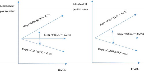
For further analysis, this study provides the partial differentiation of Model 4 (Model 7) with respect to the RIVOL (EIVOL) offers further insight on the effect of the RIVOL_CGO (EVIOL_CGO) on the likelihood of the negative relationship between RIVOL (EIVOL) and future return:

(8) $\frac{\mathrm{\partial }({\mathrm{R}}_{\mathrm{i}})}{\mathrm{\partial }(\mathrm{R}\mathrm{I}\mathrm{V}\mathrm{O}{\mathrm{L}}_{\mathrm{i}})}=0.0821+1.0850\ast \mathrm{R}\mathrm{I}\mathrm{V}\mathrm{O}\mathrm{L}\mathrm{\_}\mathrm{C}\mathrm{G}{\mathrm{O}}_{\mathrm{i}}$(8)

(9) $\frac{\mathrm{\partial }({\mathrm{R}}_{\mathrm{i}})}{\mathrm{\partial }(\mathrm{E}\mathrm{I}\mathrm{V}\mathrm{O}{\mathrm{L}}_{\mathrm{i}})}=0.0312+0.1059\ast \mathrm{E}\mathrm{I}\mathrm{V}\mathrm{O}\mathrm{L}\mathrm{\_}\mathrm{C}\mathrm{G}{\mathrm{O}}_{\mathrm{i}}$(9)

As shown in Figure 1, the slope remains negative until the CGO reaches the turning point (CGO = −0.076 for RIVOL, CGO = −0.295 for EIVOL). An increase of the IVOL starting point also increased the likelihood of positive return. Thus, the most striking result emerging from the above analysis is that the likelihood of negative return increases with dependence only when CGO is very low (embedded capital losses); in general, the relationship between IVOL (RIVOL and EIVOL) and future return are driven by the unrealized capital loss (UCL), especially the UCL1 sub-group.

Figure 1. Relationship between IVOL and likelihood of positive for various levels of CGO

3.4. Time-series regressions

In this section, the estimated alphas from time-series regressions of the UCL and UCG sub-group returns are discussed. In particular, the UCL1 and UCL2 were below and above the median unrealized capital loss (UCL), respectively. Similarly, UCG1 and UCG2 were below and above the median of unrealized capital gains (UCG), respectively. Within the UCL1, UCL2, UCG1, and UCG2 subgroups, the value-weighted (VW) and equal-weighted (EW) returns of the quintile portfolios were shaped in each month from July 1990 to June 2018 by sorting the stocks based on each of IVOL measure. The dependent variable was defined as the difference between the highest and lowest idiosyncratic volatility portfolios (H–L portfolios). Additionally, the independent variables included the excess market return (MKT), Size (SMB), and book to market (HML) following Fama and French (1993), the momentum factor (UMD) following Carhart (1997), the reverse return, and WML following Huang et al. (2010). The results are presented in Table 4 below.

Table 4. Time series regressions within Idiosyncratic Risk

	UCL1		UCL2		UCG1		UCG2
MODEL	1	2	1	2	1	2	1	2
Panel A: Realized Idiosyncratic Risk (RIVOL)
VW	−0.0763*** (−6.54)	−0.0162* (−1.94)	−0.019*** (−2.82)	0.0068 (0.41)	0.0101* (1.66)	−0.0207 (−1.01)	0.0404*** (4.60)	−0.0075 (−0.29)
EW	−0.081*** (−8.96)	−0.055** (−2.40)	−0.0232*** (−5.26)	−0.0177 (−1.31)	0.0019 (0.25)	−0.0203 (−1.18)	0.0578*** (6.04)	−0.0267 (−1.13)
Panel B: Expected Idiosyncratic Risk (EIVOL)
VW	−0.0006 (−0.06)	−0.0186 (−0.94)	0.0034 (0.68)	−0.0287 (−1.53)	0.006 (1.19)	0.0106 (0.68)	0.0069 (0.73)	−0.0131 (−0.39)
EW	−0.0166*** (−2.62)	−0.0456*** (−4.06)	0.0093** (2.30)	−0.0178 (−0.99)	0.0121** (2.05)	0.0058 (0.20)	0.0307*** (4.14)	−0.0099 (−0.39)

Equation (1)(1) ${\left(\mathrm{H}---\mathrm{L}\right)}_{\mathrm{t}}=\alpha +{\beta }_{\mathrm{M}\mathrm{K}\mathrm{T}}\mathrm{M}\mathrm{K}\mathrm{T}\mathrm{R}{\mathrm{F}}_{\mathrm{t}}+{\beta }_{\mathrm{S}\mathrm{M}\mathrm{B}}\mathrm{S}\mathrm{M}{\mathrm{B}}_{\mathrm{t}}+{\beta }_{\mathrm{H}\mathrm{M}\mathrm{L}}\mathrm{H}\mathrm{M}{\mathrm{L}}_{\mathrm{t}}+{\beta }_{\mathrm{U}\mathrm{M}\mathrm{D}}\mathrm{U}\mathrm{M}{\mathrm{D}}_{\mathrm{t}}+{\mathrm{e}}_{\mathrm{t}}$(1) shows the estimated alphas from time-series regressions of the returns of zero-investment portfolios, (H–L), using the Carhart four-factor model and Equation (2)(2) ${\left(\mathrm{H}---\mathrm{L}\right)}_{\mathrm{t}}=\alpha +{\beta }_{\mathrm{M}\mathrm{K}\mathrm{T}}\mathrm{M}\mathrm{K}\mathrm{T}\mathrm{R}{\mathrm{F}}_{\mathrm{t}}+{\beta }_{\mathrm{S}\mathrm{M}\mathrm{B}}\mathrm{S}\mathrm{M}{\mathrm{B}}_{\mathrm{t}}+{\beta }_{\mathrm{H}\mathrm{M}\mathrm{L}}\mathrm{H}\mathrm{M}{\mathrm{L}}_{\mathrm{t}}+{\beta }_{\mathrm{U}\mathrm{M}\mathrm{D}}\mathrm{U}\mathrm{M}{\mathrm{D}}_{\mathrm{t}}+{\beta }_{\mathrm{W}\mathrm{M}\mathrm{L}}\mathrm{W}\mathrm{M}{\mathrm{L}}_{\mathrm{t}-1}+{\mathrm{e}}_{\mathrm{t}}$(2) shows Carhart four-factor model and WML factor. The H-L portfolio returns are constructed as in Table 2 for the RIVOL and EIVOL. UCL1 and UCL2 are below and above median capital losses portfolios of unrealized capital loss (UCL) stocks, respectively. Similarly, UCG1 and UCG2 are below and above the median capital gains portfolios of the unrealized capital gains (UCG) stocks, respectively. Within the UCL1, UCL2, UCG1, and UCG2, the value-weighted (VW) and equal-weighted (EW) returns of the quintile portfolios were shaped in each month from July 1990 to June 2018 by sorting the stocks based on the RIVOL and EIVOL. The dependent variable is the difference between the highest and lowest idiosyncratic volatility portfolios (H–L portfolios). The independent variables include the excess market return (MKTRF), Size (SMB), book to market (HML) following Fama and French (1993), and the momentum factor (UMD) following Carhart (1997). The WML factor, estimated based on the return on a value-weighted portfolio that is long losers from the previous month and short winners from the previous month. The Newey and West (1987) adjust t-statistic is reported in the parentheses.

(1) ${\left(\mathrm{H}---\mathrm{L}\right)}_{\mathrm{t}}=\alpha +{\beta }_{\mathrm{M}\mathrm{K}\mathrm{T}}\mathrm{M}\mathrm{K}\mathrm{T}\mathrm{R}{\mathrm{F}}_{\mathrm{t}}+{\beta }_{\mathrm{S}\mathrm{M}\mathrm{B}}\mathrm{S}\mathrm{M}{\mathrm{B}}_{\mathrm{t}}+{\beta }_{\mathrm{H}\mathrm{M}\mathrm{L}}\mathrm{H}\mathrm{M}{\mathrm{L}}_{\mathrm{t}}+{\beta }_{\mathrm{U}\mathrm{M}\mathrm{D}}\mathrm{U}\mathrm{M}{\mathrm{D}}_{\mathrm{t}}+{\mathrm{e}}_{\mathrm{t}}$(1)

(2) ${\left(\mathrm{H}---\mathrm{L}\right)}_{\mathrm{t}}=\alpha +{\beta }_{\mathrm{M}\mathrm{K}\mathrm{T}}\mathrm{M}\mathrm{K}\mathrm{T}\mathrm{R}{\mathrm{F}}_{\mathrm{t}}+{\beta }_{\mathrm{S}\mathrm{M}\mathrm{B}}\mathrm{S}\mathrm{M}{\mathrm{B}}_{\mathrm{t}}+{\beta }_{\mathrm{H}\mathrm{M}\mathrm{L}}\mathrm{H}\mathrm{M}{\mathrm{L}}_{\mathrm{t}}+{\beta }_{\mathrm{U}\mathrm{M}\mathrm{D}}\mathrm{U}\mathrm{M}{\mathrm{D}}_{\mathrm{t}}+{\beta }_{\mathrm{W}\mathrm{M}\mathrm{L}}\mathrm{W}\mathrm{M}{\mathrm{L}}_{\mathrm{t}-1}+{\mathrm{e}}_{\mathrm{t}}$(2)

* Significant at the 10% level; ** Significant at the 5% level; *** Significant at the 1% level.

For the results in Panel A, the portfolio returns are sorted on the RIVOL. Within the VW and EW portfolios return shown in Model 1, the significantly negative relation between the IVOL and future return were only found in the UCL group. For example, regarding the UCL1 sub-group, the value weight (equal weight) portfolio return was −0.0763 (−0.0810) with a t-statistic −6.54 (−8.96). For UCL2 sub-group, the value weight (equal weight) portfolio return was −0.0190 (−0.0232) with a t-statistic −2.82 (−5.26). Turning to Model 2, when the return reversal factor was added, the negative significant IVOL-return still existed at a 5% level (10% level) in the VW portfolio return (EW portfolio return). Interestingly, the IVOL effect was not found in the UCG group. Thus, these results confirm the negative relationship between the idiosyncratic volatility and future return in the sample of this study, which is in line with the findings reported above.

In Panel B, the portfolio returns are sorted on the EIVOL. It can be seen that the negative IVOL-return relationship does not exist in the VW portfolios return for all CGO subgroups, which is consistent with that reported in Table 2. However, within the EW portfolios return, a negative IVOL-return relationship was found and significant at 1% level in Model 1 for the UCL1 and UCL2 sub-groups. The results obtained from the preliminary analysis of the Panel B are consistent with the findings in Table 2. Therefore, the most striking result emerging from the data is that the negative relation between the IVOL and future return concentrates on the UCL groups, rather than the UCG groups.

In general, the negative relationship between the IVOL (RIVOL and EIVOL) and future return in the UCL stocks persists after controlling for return reversal factors in the Korean stock market. Furthermore, the results from the time-series regressions and cross-sectional regression support for the hypothesis that the negative relationship between IVOL and future returns are driven by unrealized capital losses (UCL), especially the UCL1 sub-group.

4. Conclusions

This study provided an account of and the reasons for the widespread use of the negative relationship between the IVOL and future return. Moreover, this study aims to determine the concentration of negative IVOL–return relationship on the unrealized capital loss. For this purpose, the CGO was used as a reference point to divide the return into gains and losses domain. Returning to the hypothesis posed at the beginning of this study, it is now possible to state the CGO, used as described by Grinblatt and Han (2005) and Hur et al. (2010), keeps an important role to explain the negative relation between the IVOL (RIVOL and EIVOL) and future return.

One of the significant findings emerging from this study is that the unrealized capital loss was the main component driving the negative relationship between the IVOL and future returns. The empirical results were investigated by utilizing three methods, including the portfolio sort, the Fama and MacBeth (1973) regressions, and the alpha of time series regression for zero-investment portfolios. These methods provided the validation and qualification of the data and determined whether the empirical results were appropriate for the further evaluation of the objectives.

Furthermore, conclusions drawn from the present study imply that the investors have risk-seeking behaviour in the losses domain, thus, they tend to hold loose stocks too long, and then they sell them quickly in the winner position. Subsequently, these stocks are more volatility and the future return is lower. According to Grinblatt and Han (2005) and Pontiff (2006), a losing stock causes the selling pressure, the stocks are overvalued, then the market corrects the overvaluation, and the future return is negative. In line with these findings, Barberis and Xiong (2009), Hens and Vlcek (2011), and Henderson (2012) also demonstrated that investors are in their risk-averse and risk-seeking domain within a gain and loss traded, respectively. Then, they tend to hold on to the loss stocks.

Finally, the findings of this study enhance the understanding of the negative relationship between IVOL and future returns in the Korean stock market. All of these results suggest that the negative IVOL–return relationship was driven by the unrealized capital loss, meaning that investors are in their risk-seeking domain within a loss traded in the Korean market.

Additional information

Funding

The authors received no direct funding for this research.

Notes on contributors

Nguyen Truong Son

Le Thi Minh Hang is a lecturer at the University of Economics, University of Da Nang. Her research interests lie in asset pricing in emerging markets, and development finance focused on supply chain financing. Hoang Van Hai is a lecturer at the University of Economics, University of Da Nang. His key research interests are on asset pricing in emerging financial markets, macroeconomics, and international economics. Nguyen Truong Son is a lecturer at the University of Economics, University of Da Nang. His research interests are capital markets, asset pricing, and higher education.

References

- An, L., Wang, H., Wang, J., & Yu, J. (2017). Lottery-related anomalies: The role of reference-dependent preferences. PBCSF-NIFR Research Paper No. 15-04. SSRN. https://ssrn.com/abstract=2636610.
- Ang, A., Hodrick, R., Xing, Y., & Zhang, X. (2006). The cross-section of volatility and expected returns. Journal of Finance, 61(1), 259–15. https://doi.org/10.1111/j.1540-6261.2006.00836.x
- Ang, A., Hodrick, R. J., Xing, Y., & Zhang, X. (2009). High idiosyncratic volatility and low returns: International and further u.S. Evidence. Journal of Financial Economics, 91(1), 1–23. https://doi.org/10.1016/j.jfineco.2007.12.005
- Bali, T. G., Cakici, N., & Whitelaw, R. F. (2011). Maxing out: Stocks as lotteries and the cross-section of expected returns. Journal of Financial Economics, 99(2), 427–446. https://doi.org/10.1016/j.jfineco.2010.08.014
- Barberis, N., & Huang, M. (2008). Stocks as lotteries: The implications of probability weighting for security prices. American Economic Review, 98(5), 2066–2100. https://doi.org/10.1257/aer.98.5.2066
- Barberis, N., Huang, M., & Santos, T. (2001). Prospect theory and asset prices. The Quarterly Journal of Economics, 116(1), 1–53. https://doi.org/10.1162/003355301556310
- Barberis, N., & Xiong, W. (2009). What drives the disposition effect? An analysis of a long-standing preference-based explanation. Journal of Finance, 64(2), 751–784. https://doi.org/10.1111/j.1540-6261.2009.01448.x
- Barberis, N. C. (2013). Thirty years of prospect theory in economics: A review and assessment. Journal of Economic Perspectives, 27(1), 173–196. https://doi.org/10.1257/jep.27.1.173
- Boyer, B., Mitton, T., & Vorkink, K. (2010). Expected idiosyncratic skewness. The Review of Financial Studies, 23(1), 169–202. https://doi.org/10.1093/rfs/hhp041
- Carhart, M. (1997). On persistence in mutual fund performance. Journal of Finance, 52(1), 57–82. https://doi.org/10.1111/j.1540-6261.1997.tb03808.x
- Chichernea, D. C., Kassa, H., & Slezak, S. L. (2019). Lottery preferences and the idiosyncratic volatility puzzle. European Financial Management, 25(3), 655–683. https://doi.org/10.1111/eufm.12178
- Fama, E., & French, K. (1993). Common risk factors in the returns on stocks and bonds. Journal of Financial Economics, 33(1), 3–56. https://doi.org/10.1016/0304-405X(93)90023-5
- Fama, E., & MacBeth, J. D. (1973). Risk, return, and equilibrium: Empirical tests. Journal of Political Economy, 81(3), 607–636. https://doi.org/10.1086/260061
- Frazzini, A. (2006). The disposition effect and underreaction to news. Journal of Finance, 61(4), 2017–2046. https://doi.org/10.1111/j.1540-6261.2006.00896.x
- Fu, F. (2009). Idiosyncratic risk and the cross-section of expected stock returns. Journal of Financial Economics, 91(1), 24–37. https://doi.org/10.1016/j.jfineco.2008.02.003
- Grinblatt, M., & Han, B. (2005). Prospect theory, mental accounting, and momentum. Journal of Financial Economics, 78(2), 311–339. https://doi.org/10.1016/j.jfineco.2004.10.006
- Harris, L. (1988). Predicting contemporary volume with historic volume at differential price levels: Evidence supporting the disposition effect: Discussion. Journal of Finance, 43(3), 698–699. DOI: 10.2307/2328192
- Henderson, V. (2012). Prospect theory, liquidation, and the disposition effect. Management Science, 58(2), 445–460. https://doi.org/10.1287/mnsc.1110.1468
- Hens, T., & Vlcek, M. (2011). Does prospect theory explain the disposition effect? Journal of Behavioral Finance, 12(3), 141–157. https://doi.org/10.1080/15427560.2011.601976
- Huang, W., Liu, Q., Rhee, S. G., & Zhang, L. (2010). Return reversals, idiosyncratic risk, and expected returns. Review of Financial Studies, 23(1), 147–168. https://doi.org/10.1093/rfs/hhp015
- Hur, J., Pritamani, M., & Sharma, V. (2010). Momentum and the disposition effect: The role of individual investors. Financial Management, 39(3), 1155–1176. https://doi.org/10.1111/j.1755-053X.2010.01107.x
- Ingersoll, J. E., & Jin, L. J. (2013). Realization utility with reference-dependent preferences. The Review of Financial Studies, 64(3), 723–767. https://doi.org/10.1093/rfs/hhs116
- Kaustia, M. (2010). Prospect theory and the disposition effect. Journal of Financial and Quantitative Analysis, 45(3), 791–812. https://doi.org/10.1017/S0022109010000244
- Lakonishok, J., & Smidt, S. (1986). Volume for winners and losers: Taxation and other motives for stock trading. Journal of Finance, 41(4), 951–974. https://doi.org/10.1111/j.1540-6261.1986.tb04559.x
- Merton, R. (1987). A simple model of capital market equilibrium with incomplete information. Journal of Finance, 42(3), 483–510. https://doi.org/10.1111/j.1540-6261.1987.tb04565.x
- Nartea, G., Wu, J., & Liu, H. T. (2014). Extreme returns in emerging stock markets: Evidence of a max effect in south korea. Applied Financial Economics, 24(6), 425–435. https://doi.org/10.1080/09603107.2014.884696
- Newey, W., & West, K. (1987). A simple, positive semi-definite, heteroskedasticity and autocorrelation consistent covariance matrix. Econometrica, 55(3), 703–708. DOI: 10.2307/1913610
- Odean, T. (1998). Are investors reluctant to realize their losses? Journal of Finance, 53(5), 1775–1798. https://doi.org/10.1111/0022-1082.00072
- Peterson, D. R., & Smedema, A. R. (2011). The return impact of realized and expected idiosyncratic volatility. Journal of Banking and Finance, 35(10), 2547–2558. https://doi.org/10.1016/j.jbankfin.2011.02.015
- Pontiff, J. (2006). Costly arbitrage and the myth of idiosyncratic risk. Journal of Accounting and Economics, 42(1–2), 35–52. https://doi.org/10.1016/j.jacceco.2006.04.002
- Thaler, R., & Johnson, E. J. (1990). Gambling with the house money and trying to break even: The effects of prior outcomes on risky choice. Management Science, 36(6), 643–660. https://doi.org/10.1287/mnsc.36.6.643
- Tversky, A., & Kahneman, D. (1979). Prospect theory: An analysis of decision under risk. David K. Levine. Levine's Working Paper Archive.
- Tversky, A., & Kahneman, D. (1992). Advances in prospect theory: Cumulative representation of uncertainty. Journal of Risk and Uncertainty, 5(4), 297–323. https://doi.org/10.1007/BF00122574
- Wang, H., Yan, J., & Yu, J. (2017). Reference-dependent preferences and the risk–return trade-off. Journal of Financial Economics, 123(2), 395–414. https://doi.org/10.1016/j.jfineco.2016.09.010