Asymmetric effect of monetary policy on Indian stock market sectors: Do monetary policy stimulus transpire the same effect on all sectors?

Abstract

Most studies for the monetary policy effect on stock markets have concentrated on using the primary index to proxy the stock market. The present paper, avoiding “aggregation bias”, seeks to unbundle the effect of monetary policy on the stock market in two ways. First, the non-linear model is used. Second, sector-level monetary policy variable association and strength is known. Nonlinear Auto-Regressive Distributed Lag method (NARDL) has been used to separate the effect of monetary policy implications. The positive and negative separation of monetary policy variables shows meaningful information relating to each sector. Furthermore, the NARDL model provides the Error Correction equation for future prediction of the sector performance. The Error Correction Term (ECT) is significant for all the sectors, besides Information Technology. While ECT is highest for the Power sector, the lowest is reported for the Metal sector. Inflation increase has substantially more effect on sectors then its decrease. For short-run, real exchange rate positive (REER_POS (−2)), with a lag of 2 months, is effective for all the sectors. The health care sector stands out in its sensitivity to monetary policy variables. The asymmetric response of the Sector equity markets to monetary policy variables throws new insight for the policymakers, business managers, and fund managers. The nonlinearity can be helpful for business managers to relate revenue and valuation to monetary policy. Likewise, the portfolio fund managers can prepare for the expected changes in the economy to reallocate and rebalance their portfolios.

Keywords:

• Non-linear Model
• monetary policy asymmetric effectiveness
• sectoral stock market
• Bombay stock exchange India

PUBLIC INTEREST STATEMENT

Monetary Policy affects all of us today. With the availability of the latest information, we can foresee and manage our consumption and savings better. For example, suppose inflation increases by 1%. In that case, our savings will no longer buy the same amount of products/services we intend to believe in in the future. Therefore, the loss of investment returns is easily assessed. However, suppose inflation decreases by 1%. In that case, stock returns may not increase with the same percentage as returns decreased due to a 1% increase in inflation. The asymmetry hence is highlighted by using the new technique of NRADL. This article helps show how each industrial sector equity market acts very different from the other. Monetary policy variables such as inflation, interest rates, money supply and exchange rates impact are evaluated on 14 sectors. Each variable is compared to its own increase decrease effect on each sector. This adds to the multidimensional information availability for each industry.

1. Introduction

Any economy to thrive needs a conducive social, political, and economic environment. Providing economic growth environment is the responsibility of the Government and Central Bank. While Central Bank controls the overall monetary policy, Government regulates the fiscal policy. (Erduman et al., 2020) Monetary policy uses tools like Interest rates, liquidity management, exchange rate, credit creation and money supply to nurture the economy. Any deviations from the objective are corrected. For example, suppose inflation starts to reach beyond the favourable limits. In that case, the Central bank will increase interest rates, making borrowing expensive for the consumers and hence curtails more demand in the economy. As inflation and interest rates will also affect the output levels in the economy, the stock market will be affected too. Financial markets provide price discovery mechanism by discounting the future earnings of firms(Elgammal et al., 2020). The general economic and financial theory explains that the efficient financial market will value stock prices more when expected earnings are good. In simple terms, the more a firm is expected to earn more valuable will be the firm’s equity share (stock price) prices. The financial markets are, however, very information sensitive. The very anticipation of possible monetary policy announcements by central bank impacts the markets. (Sehgal et al., 2015) The relation of Equity markets and monetary policy is still being debated for what causes or influence what? These interactions of the economy and financial markets are strong enough to impact for a long time. (Gopinath et al., 2020; Kim, 2003; Richards et al., 2009) For example, Japan witnessed a sluggish economy for 10 years after the collapse of the Japanese stock market in the 1990s (Mishkin & White, Mishkin and White,). The relation of the stock market and monetary policy is far more complex than standard theory would explain. Hence, what is needed is a more intense evaluation of the channel of impulse from monetary policy to the stock market or vice versa. Bernanke and Gertler (1995) referred to this path as the “Black Box”. They have urged that what is needed is to understand the clarity of this transmission path.

In the last decade, the availability of better data sets and user-friendly statistical packages have helped researchers find better insights into this conduit of monetary policy and stock markets. Good examples are extension of earlier work, such as by Victor (Caldara & Herbst, 2019; Ramey, 2011; Barro & Redlick, 2011; Romer & Romer, 2004; Zarnowitz, Zarnowitz, 1985). In addition, the recent works brings out the asymmetric interaction of the monetary policy by relaxing the assumption of linearity. (Caldara & Herbst, 2019; King, 2011; Miranda-Agrippino et al., 2016; Ng & Wright, 2013)

Nevertheless, there is a dearth of such studies for developing countries like India, which is an unfilled research gap. This study hence undertakes to fill this gap. The present paper will assess if these monetary variables have an asymmetric impact on India’s stock market sectors.

Plan of the paper. Section 1.1 explains the target-dependent variable, the “sector indices”. Section 2 covers each explanatory variable’s theoretical framework and related literature review. The peculiarity of economic and financial data is discussed to select the NARDL Model used. The result and discussion follow the section of data and methodology. Finally, the conclusion and policy implication are followed by research limitation and further research potential.

1.1. Why sectoral equity indices?

Figure 1 shows the returns of all 15 sectors and the primary index of Bombay Stock Exchange “Sensex” named BSE in the chart. Figure 1 shows how sectoral returns differ. The best returns are given by FMCG (16.3%) sector and the worst by the Reality sector (−13.4%). (CAGR Compounded Annual Growth Rate)

Figure 1. Sectoral Equity CAGR

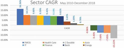
The industries have their specific business nature and uniqueness. Similar revenue of a steel manufacturer and a software company will have very different fixed assets, working capital profitability and expense ratios. Hence the risk-return profiles differ. The difference of each industrial sector calls for different treatment by the economic policymakers, fund managers and business managers. The mutual fund managers and investment bankers keep rebalancing their funds exposure to different asset class and industrial sectors. The motive of portfolio diversification is mainly to reduce risk without sacrificing return (Efficient Portfolio). Much of the academic debate is based on deciding the premises of diversification strategy. The sector is one of the most used bases of diversification (Aw et al., 2018; Hughen & Strauss, 2017; Kumar, 2019). Using sector-level data as the target variable will hence benefit the objective of the research in many ways. First, the sector-level data will disaggregate the impact of monetary variables as positive and negative affect. For example, it will be known that if the interest rates (Government Bond yields) will affect all the sectors similarly (symmetric) or differently (asymmetric). Answering questions like, “Do all the sectors provide equal protection against inflation?” The present paper will try to find if all the variables as explanatory variables have a differential effect on each sector. Secondly short-run impact of monetary policy will be known with its lags and asymmetry. Third, the paper seeks to know if the long-term impact of explanatory variables is more substantial than the short term. Fourthly this paper seeks to know if the long-term relationship is established from explanatory variables to target variables; if so, can the predictive equation be formed?

2. Theoretical background and literature review

The earliest work on sector-level data or avoiding the aggregation bias” is by Soenen and Hennigar (1988). Enlarging the set of variables to a broader set from market index to sectoral index were the works by (Bahmani-Oskooee & Saha, Bahmani-Oskooee and Saha, 2016a; Chatziantoniou et al., 2020; Mitra, 2008; Tiryaki et al., 2018) who used sector-level data as target variables. Similarly, Bahmani and Mitra used data of 40 industries to find trade between India and the US. While (Joshi & Giri, 2015; Pal & Garg, 2019) have used sector data using VAR, VECM, GMM and ARDL to analyze the data. The nonlinearity has not been used.

2.1. Inflation

The most crucial objective for a central bank is the effective control of inflation. The inflation target set by Central Banks is generally set to vary within a range. For example, the RBI (Reserve Bank of India or the Central Bank of India) targets 4% inflation with a tolerance of ±2%. In India, the “flexible inflation target” was adopted in 2015. (RBI uses Consumer Price index or CPI instead of WPI or Wholesale Price index since 2014) (Alqaralleh, 2020).

General theory connects stock market and inflation. Fisher’s hypothesis advocates that inflation and stock markets are directly related (Jaffe & Mandelker, 1979; Singh & Balasubramanian, 2020). If the markets are efficient, the stock prices will reflect the information (Fama, 1970; Gurmeet, 2020; Singh, et al., 2020). The theory explains that an increase in inflation will reduce the interest rates earned by the fixed income instruments investors (Bonds, Fixed Deposits) (Baele et al., 2020; Bozhkov et al., 2020; Corbet et al., 2021). This is because as the Interest earned is fixed, and the purchasing power of the investors decreases. Inflation also decreases the real return for equity investors. Investors reallocate their savings as they deplete in value for better returns (Singh & Padmakumari, 2020). Another link between inflation and the stock market is proposed from the producer’s point of view. The borrowing costs will increase for the industry; exports become less competitive, business uncertainty increases, increasing the discounts rates and depleting the market value of firms. However, research finds mixed support for Fisher's hypothesis. For example, the research not confirming to Fisher are (Gallagher & Taylor, 2002; Gregoriou & Kontonikas, 2010; Gultekin & Gultekin, 1983; Li et al., 2016; Omay et al., 2015; Worthington & Pahlavani, 2007). Alqaralleh explains that this conflict is because of the linearity assumption(Alqaralleh, 2020). The data used in economics and finance are non-linear (Alqaralleh, 2020 Boswijk, Hommes & Manzan, 2007; Brock & Hommes, 1998; Iddrisu & Alagidede, 2020; Sathyanarayana & Gargesa, 2018; Alqaralleh, 2020). More India-specific study by Raghutla et al. (2020) found a significant negative relation between inflation and output and a positive relation between output and stock price. (Chatrath et al., 1996; Magweva & Sibanda, 2020) find partial support for Fama’s hypothesis Boswijk, et al., 2007

2.2. Exchange rate

Two theoretical models explain the relation of exchange rate and the stock market. The first model (flow-oriented model or traditional approach) by Dornbusch and Fischer (1980) explains that the changes in the exchange rates will make the country’s product globally competitive through the output, thereby leading to change in the stock market. This model considers that if the exchange rates depreciate (home currency depreciates), the exports become more attractive globally and similarly the opposite effect for exchange rate appreciation. Thus, the direction of effect is from the exchange rate to stock prices. Supporting literature are by (C.-C. Nieh & Yau, 2004; Lin & Fu, 2016; Phylaktis & Ravazzolo, 2005; Sui & Sun, 2016; Yang et al., 2017).

The other model is the “stock-oriented model” by Branson (Fernández-Rodríguez & Sosvilla-Rivero, 2020, 1983Fernández-Rodríguez and Sosvilla-Rivero, 2020) and Frankel (1983). This model suggests that when the domestic market becomes more attractive to foreign investors, foreign capital flows in the domestic stock market, leading to appreciation of domestic currency (Long et al., 2021). Conversely, a decline in the stock prices will erode the investor’s wealth, making interest rates decline and reducing the demand for money. In addition, the decline of stock values in the domestic market leads to capital outflow to foreign markets, declining the exchange rates. As a result, fund managers actively reallocate and rebalance their funds. (Bahmani-Oskooee & Saha, Bahmani-Oskooee and Saha, 2016b)

Research literature that finds ambiguous relation between exchange rate and stock prices are (Bahmani-Oskooee & Sohrabian, 1992; C.C. Nieh & Lee, 2001; Doong et al., 2005; Fernández-Rodríguez & Sosvilla-Rivero, 2020; Kollias et al., 2012; Rahman & Uddin, 2009; Smyth & Nandha, 2003; Wu, 2000; Zhao, 2010).

2.3. Interest rates

The Monetary policy uses interest rates, among other tools, to achieve its growth and stability objectives. The theoretical framework provides that the interest rates channel flowing from monetary policy to the stock market affects investment and aggregate output or inflation (Boivin et al., 2010; Iddrisu & Alagidede, 2020; Mishkin, 1996). Moreover, the impact propagates indirectly from monetary policy to the stock market. For example, the increase in the interest rates makes bank savings, bonds more attractive, and capital flows from equity markets to bond markets. Although these links of monetary policy and interest rates are more complex than the simple theory explains. However, the research by Flannery and James (1984), Sweeney and Warga (1986) find interest rate and stock market negatively related (Elliott et al., 2014). Kuenen et al., () finds interest rates and assets return correlation increases during the crisis. As a result, there is hesitancy among the investors to opt for assets, and the stock market follows a trend (Sandoval & Franca, 2012). Acosta-González, et al., 2012In contrast, the study by Czaja et al. (2009) and Korkeamäki (2011)shows the weakening impact of interest rates on the stock markets over the period. This they attribute to the better risk mitigating tools available.

2.4. Money supply

The Monetarist and Keynesian view that the money supply can affect equity stock prices through monetary policy. As per the monetarist, stock prices increase due to expansionary monetary policy. Increasing the optimum money supply increases the demand for equities. While the Keynesian theory forwards the argument that a decrease in interest rates (an expansionary monetary policy) makes the fixed income instruments (bonds) less attractive than equities. The flow of impact from money supply to stock prices is also indirectly moving through other channels. An increase in money supply leads to a decrease in the interest rates, increase in investment and GDP leading to stock price appreciation (Tiryaki et al., 2018)

One of the earliest works to link money supply with stock markets is that by (Altintas & Yacouba, 2018; Hamburger & Kochin, 1972; Sprinkel, 1964). For this ongoing debate, Fama (1981) argues that inflation will increase as the money supply increases, decreasing stock prices. Differing from above (Kumar & Padhi, 2012; Kwon & Shin, 1999; Ratanapakorn & Sharma, 2007) find a positive relation between stock prices and money supply. However, some research literature supports both of the above views. (Blume et al., 1977; Hanousek & Filer, 2000; Husain et al., 1999; Rozeff, 1974; Tiryaki et al., 2018) find long term declining cointegration link between money supply and stock market over the period of time.

2.5. Non-linearity of finance and economic data

Much of the conflicting literature of monetary policy variables and stock market relation is because of linearity assumption (Boswijk, Hommes & Manzan, 2007; Brock & Hommes, 1998) As Alqaralleh explains, data used in economics and finance are non-linear. For inflation, the nonlinearity robustness as assumption can be the financial crisis, spurt of deflation, or inflation, which alters the relation of inflation and stock markets (see, among others, Bahoul, Mroua & Naifar, 2017; Bildirici & Türkmen, 2015; Rocher, 2017). The problem with the symmetric assumption of exchange rate impact on stock markets is that it may understate the impact (Effiong & Bassey, 2019; Salisu et al., 2020; Wong, 2019). Kassi, et al., 2019 points out th Ding, et al., 2019at the relation of exchange rate and stock prices varies with time, and the linear models may not be an excellent model to find the relation of the variables (Si et al., 2021). More such studies that point out the inadequacy of linear models are (Ismail & Isa, 2009) by Ismail and Isa, Bahmani—Saha (Bahmani-Oskooee & Saha, Bahmani-Oskooee and Saha, 2016b)

3. Data and methodology

The data used is from May 2010 to December 2018. The reason for choosing the data time is as follows. The Indian Central bank—Reserve Bank of India had undergone a paradigm shift in monetary policy formulation and functioning. Parallel to the policy shift, certain events also had a profound impact on the Indian economy. These events were high inflation (2011), national election (2014), and demonetisation (2016) (Chatziantoniou et al., 2020).

Data used: The Independent variables for the present study are (data from Reserve Bank of India) Consumer Price Index, REER (Real Effective Exchange Rate), Broad Money M3, Interest rates (yield of SGL or the subsidiary general ledger of India’s Government traded securities). The SGL accounts yields have been used as it accounts for nearly 98% of government securities trade and is the primary tool for the central bank to regulate the liquidity in the economy (“Download Reports | Ministry of Statistics and Program Implementation | Government Of India,” n.d.).

For the Stock market, 15 sectors are used from Bombay Stock Exchange Indices. In addition, the Bombay Stock Exchange has 20 industry-based indices. The data, however, is not available for all the sectors from 2010 onwards. Hence, only those sectors are used for which the data is available for the study period. The sectors are Automobile, Bank, Consumer Durable, Capital Goods, Energy, Finance, Health care, Material, Oil & Gas, Power, Reality, Telecom, Fast Moving Consumer Goods, Metal, Information Technology.

4. Methodology

The NARDL model is an asymmetric extension of the linear ARDL model extended by Pesaran and Shin (1999) and Pesaran et al. (2001). The unrestricted error correction model in the linear ARDL model takes the following forms:

(1) $\mathrm{\Delta }{y}_t={\delta }_0+\sigma y_{t-1}+\vartheta x_{t-1}+\sum _{i=1}^{p-1}{\mu }_i\mathrm{\Delta }{y}_{t-i}+\sum _{i=0}^{q-1}{\beta }_i{x}_{t-i}+{\epsilon }_t$(1)

Here $y_t$ is the dependent variable, while $x_{t}isakx1$ vector of regressors. The parameters of $\sigma$ and $\vartheta$ represent the long run and the parameters of ${\mu }_i$ and ${\beta }_i$ represent the short-run coefficients, respectively. The ${\epsilon }_t$ is the error term.

The NARDL decomposes the vector of regressor ($x_t$) into its positive and negative partial sums. The decomposition $x_t$ of the can be written as follows:

(2) $x_t=x_0+x_t^{+}+x_t^{-}$(2)

In equation (2)(2) $x_t=x_0+x_t^{+}+x_t^{-}$(2) , $x_0$ is the initial value

$x_t^{+}=\sum _{i=1}^t\mathrm{\Delta }{\mathrm{x}}_i^{+}\sum _{i=1}^{t}max\left(\mathrm{\Delta }{x}_i,0\right)and{x}_t^{-}=\sum _{i=1}^t\mathrm{\Delta }{\mathrm{x}}_i^{-}=\sum _{i=1}^{t}min\left(\mathrm{\Delta }{x}_i,0\right)$ are the positive and negative partial sums.

Non-linear asymmetric long-run cointegrating regression in the NARDL model is written as:

(3) $y_t={\lambda }^{+}{x}_t^{+}+{\lambda }^{-}{x}_t^{-}+e_t$(3)

In equation (3)(3) $y_t={\lambda }^{+}{x}_t^{+}+{\lambda }^{-}{x}_t^{-}+e_t$(3) , $e_t$ denotes the deviation from the long-run equilibrium. While ${\lambda }^{+}$ and ${\lambda }^{-}$ represent the long-run coefficients associated with the positive and negative changes in $x_t$, respectively. Hence, the asymmetric error correction model can be written as by combining equations (1)(1) $\mathrm{\Delta }{y}_t={\delta }_0+\sigma y_{t-1}+\vartheta x_{t-1}+\sum _{i=1}^{p-1}{\mu }_i\mathrm{\Delta }{y}_{t-i}+\sum _{i=0}^{q-1}{\beta }_i{x}_{t-i}+{\epsilon }_t$(1) and (3(3) $y_t={\lambda }^{+}{x}_t^{+}+{\lambda }^{-}{x}_t^{-}+e_t$(3) ) as follows:

(4) $\mathrm{\Delta }{y}_t={\delta }_0+\sigma y_{t-1}+{\vartheta }^{+}{x}_{t-1}^{+}+{\vartheta }^{-}{x}_{t-1}^{-}\sum _{i=1}^{p-1}{\mu }_i\mathrm{\Delta }{y}_{t-i}+\sum _{i=0}^{q-1}({\beta }_i^{+}\mathrm{\Delta }{x}_{t-i}^{+}+{\beta }_i^{-}\mathrm{\Delta }{x}_{t-i}^{-})+{\epsilon }_t$(4)

In equation (4)(4) $\mathrm{\Delta }{y}_t={\delta }_0+\sigma y_{t-1}+{\vartheta }^{+}{x}_{t-1}^{+}+{\vartheta }^{-}{x}_{t-1}^{-}\sum _{i=1}^{p-1}{\mu }_i\mathrm{\Delta }{y}_{t-i}+\sum _{i=0}^{q-1}({\beta }_i^{+}\mathrm{\Delta }{x}_{t-i}^{+}+{\beta }_i^{-}\mathrm{\Delta }{x}_{t-i}^{-})+{\epsilon }_t$(4) above dependent and explanatory variables are both defined as ${\vartheta }^{+}=-\sigma {\lambda }^{+}$ and ${\vartheta }^{-}=-\sigma {\lambda }^{-}$, and ${\beta }_i^{+}$ and ${\beta }_i^{-}$ are the short-run adjustments to positive and negative changes in the explanatory variables $x_t$.

Following Shin, Shin and Greenwood-Nimmo (2014) in order to test the short-run long-run asymmetric effects of CPI, REER, M3, and Interest rates on indices returns, the NARDL model has to take the following steps. First, equation (4)(4) $\mathrm{\Delta }{y}_t={\delta }_0+\sigma y_{t-1}+{\vartheta }^{+}{x}_{t-1}^{+}+{\vartheta }^{-}{x}_{t-1}^{-}\sum _{i=1}^{p-1}{\mu }_i\mathrm{\Delta }{y}_{t-i}+\sum _{i=0}^{q-1}({\beta }_i^{+}\mathrm{\Delta }{x}_{t-i}^{+}+{\beta }_i^{-}\mathrm{\Delta }{x}_{t-i}^{-})+{\epsilon }_t$(4) should be estimated by standard OLS. Second, the bond test approach can be applied by using the F-statistics (F_PSS) developed by Pesaran et al. (2001) to test the existence of asymmetric long-run relationship among the levels of the series $y_t$, $x_t^{+}$, $x_t^{-}$. Thus, F_PSS refers to the joint null hypothesis of no cointegration. It can be expressed as:

(5) $H_0:\sigma ={\vartheta }^{+}={\vartheta }^{-}=0$(5)

(6) $H_1:\sigma \ne {\vartheta }^{+}\ne {\vartheta }^{-}\ne 0$(6)

Third the null hypothesis is $\vartheta ={\vartheta }^{+}={\vartheta }^{-}$ for the long-run symmetry and $\sum _{i=0}^{q-1}{\beta }^{+}$ $\sum _{i=0}^{q-1}{\beta }^{-}$ for the short-run symmetry is tested by employing the Wald test. Fourth, equation (4)(4) $\mathrm{\Delta }{y}_t={\delta }_0+\sigma y_{t-1}+{\vartheta }^{+}{x}_{t-1}^{+}+{\vartheta }^{-}{x}_{t-1}^{-}\sum _{i=1}^{p-1}{\mu }_i\mathrm{\Delta }{y}_{t-i}+\sum _{i=0}^{q-1}({\beta }_i^{+}\mathrm{\Delta }{x}_{t-i}^{+}+{\beta }_i^{-}\mathrm{\Delta }{x}_{t-i}^{-})+{\epsilon }_t$(4) is utilised to derive asymmetric cumulative dynamic multipliers effect on $y_t$, of the change in $x_t^{+}$ and $x_t^{-}$.

The same can be expressed as:

(7) $m_h^{+}=\sum _{j=0}^h\frac{\mathrm{\partial }{y}_{t+j}}{\mathrm{\partial }{x}_t^{+}},\mathrm{a}\mathrm{n}\mathrm{d}{m}_h^{-}=\sum _{j=0}^h\frac{\mathrm{\partial }{y}_{t+j}}{\mathrm{\partial }{x}_t^{-}}$(7)

Where (h = 0,1,2 ….). For equation (7)(7) $m_h^{+}=\sum _{j=0}^h\frac{\mathrm{\partial }{y}_{t+j}}{\mathrm{\partial }{x}_t^{+}},\mathrm{a}\mathrm{n}\mathrm{d}{m}_h^{-}=\sum _{j=0}^h\frac{\mathrm{\partial }{y}_{t+j}}{\mathrm{\partial }{x}_t^{-}}$(7) , if h $\to \mathrm{\infty },$ then $m_h^{+}\to {\lambda }^{+}$ and $m_h^{+}\to {\lambda }^{+}$, the long run coefficients of ${\lambda }^{+}$ and ${\lambda }^{-}$ are computed as

(8) ${\lambda }^{+}=-\frac{{\vartheta }^{+}}{\sigma }\mathrm{a}\mathrm{n}\mathrm{d}{\lambda }^{-}=-\frac{{\vartheta }^{-}}{\sigma }$(8)

The study estimated the NARDL model covering the short run and long run of the positive and negative partial sums. Thus, the NARDL model takes the following equation form:

(9) $\begin{array}{rl}& \mathrm{\Delta }Lnsectorinde{x}_t={\delta }_0+\sigma lnsectoride{x}_{t-1}+{\vartheta }_1^{+}CP{I}_{t-1}^{+}+{\vartheta }_1^{-}CP{I}_{t-1}^{-}+{\vartheta }_2^{+}lninterestrat{e}_{t-1}^{+}\\ & +{\vartheta }_2^{-}lninterestrat{e}_{t-1}^{-}+{\vartheta }_3^{+}M{3}_{t-1}^{+}+{\vartheta }_3^{-}M{3}_{t-1}^{-}+{\vartheta }_4^{+}REE{R}_{t-1}^{+}+{\vartheta }_4^{-}REE{R}_{t-1}^{-}+\sum _{i=1}^{p-1}{\mu }_i\mathrm{\Delta }lnsectorinde{x}_{t-i}\\ & +{\sum }_{i=0}^q{\beta }_{1,i}^{+}\mathrm{\Delta }CP{I}_{t-1}^{+}+{\sum }_{i=0}^q{\beta }_{1,i}^{-}\mathrm{\Delta }CP{I}_{t-1}^{-}+{\sum }_{i=0}^q{\beta }_{2,i}^{+}\mathrm{\Delta }lninterestrat{e}_{t-1}^{+}\\ & +{\sum }_{i=0}^q{\beta }_{2,i}^{-}\mathrm{\Delta }lninterestrat{e}_{t-1}^{-}+{\sum }_{i=0}^q{\beta }_{3,i}^{+}\mathrm{\Delta }M{3}_{t-1}^{+}+{\sum }_{i=0}^q{\beta }_{3,i}^{-}\mathrm{\Delta }M{3}_{t-1}^{-}+{\sum }_{i=0}^q{\beta }_{4,i}^{+}\mathrm{\Delta }REE{R}_{t-1}^{+}\\ & +{\sum }_{i=0}^q{\beta }_{4,i}^{-}\mathrm{\Delta }REE{R}_{t-1}^{-}+{\epsilon }_t\end{array}$(9)

Equation 1(1) $\mathrm{\Delta }{y}_t={\delta }_0+\sigma y_{t-1}+\vartheta x_{t-1}+\sum _{i=1}^{p-1}{\mu }_i\mathrm{\Delta }{y}_{t-i}+\sum _{i=0}^{q-1}{\beta }_i{x}_{t-i}+{\epsilon }_t$(1) , y_t is the dependent variable, while x_t includes all sets of regressors (set vectors k*1) and α0 as intercept. Difference operator as ∆. Short-run coefficients are b₁,c₁. Long run coefficients: ρ and θ. The lag operators are p and q. The null hypothesis for NARDL (non-linear autoregressive distributed lag) testing of cointegrating is ρ = θ = 0 while the alternate hypothesis is ρ ≠ θ ≠ 0. As per shin (Shin & Greenwood-nimmo, 2013), if F statistics are above the upper bound, the long-run cointegration is found in the model.

5. Result and discussion

After confirming that all variables unit root are either I(0) or I(1), (Table 1) but not I(2) NARDL equations formed pass through Breusch–Godfrey Serial Correlation LM Test, Heteroskedasticity Test: Ramsey RESET Test and Normality test (Table 2). All models pass the bounds test at P-Value 5% to 10% besides IT which is dropped from further evaluation. The model results are evaluated hereafter.

Table 1. Unit root test

Test	Auto	Bank	CD	CG	Energy	Finance	FMCG	HC	Material
ADF I(0)	−1.3426	−0.7436	−0.4588	−1.2589	−0.5974	−0.6387	−1.6857	−1.6704	−0.9034
ADF I(1)	−10.1662***	−9.8306***	−9.2962***	−9.197***	−12.6023***	−9.1106***	−12.0857***	−11.345***	−9.7292***
PP I(0)	−1.33	−0.5763	−0.4117	−1.2869	−0.3337	−0.5667	−2.0107	−1.6704	−0.9051
PP I(1)	−10.1113***	−9.8571***	−9.3468***	−9.1967***	−11.3218***	−9.1378***	−11.7841***	−11.1652***	−9.7393***
Test	Metal	OG	Power	Reality	Telecom	CPI	INTEREST	M3	REER
ADF I(0)	−2.2145	−1.0305	−2.687*	−2.7716*	−2.6137*	−3.9927***	−2.1949	−5.3334***	−2.3099
ADF I(1)	−9.832***	−11.1056***	−10.7757***	−9.7606***	−12.5181***	−8.1606***	−12.0515***	−9.6156***	−7.6138***
PP I(0)	−2.2818	−0.8557	−2.6114*	−2.8004*	−2.4717	−2.9337**	−2.0872	−16.0902***	−2.1656
PP I(1)	−9.8192***	−11.0258***	−10.5508***	−9.6947***	−12.4604***	−7.8191***	−12.0811***	−6.7068***	−7.5981***

*Significant at the 10%; **significant at the 5%; ***significant at the 1% and (no) not significant.

Lag length based on SIC; ADF: Augmented Dickey Fuller Test; PP: Phillips Perron Test

Table 2. Model dignostics test

Sectors	Auto	Bank	CD	CG	Energy	Finance	FMCG	HC	Material	Metal	OG	Power	Reality	Telecom
Coint Eq(−1) Coefficient	−0.233***	−0.299***	−0.251***	−0.26***	−0.326***	−0.284***	−0.353***	−0.297***	−0.287***	−0.224***	−0.338***	−0.388***	−0.287***	−0.269***
Normality Test P-value	0.42***	0.613***	0.778***	0.518***	0.264***	0.789***	0.48***	0.712***	0.241***	0.557***	0.514***	0.467***	0.277***	0.433***
Serial Correlation LM Test	0.946	0.604	0.762	0.564	0.28	0.527	0.808	0.073	0.726	0.394	0.164	0.489	0.949	0.208
Ramsey RESET Test T statistics	0.178	0.6715	0.3535	0.9866	0.3808	0.926	0.763	0.246	0.113	0.736	0.858	0.273	0.394	0.217
Bound TestF Statistics & P Value	3.3*	5.0***	4.2***	4.7***	4.4***	5.1***	3.1*	4.4***	4.2***	3.0*	4.5***	5.1***	4.3***	3.4**

*Significant at the 10%; **significant at the 5%; ***significant at the 1% and (no) not significant.

The cointegration equation (ECT – Error Correction Term) to be meaningful needs to be statistically significant, less than 1 and negative (Pesaran et al., 2001), which all sectors verify (Table 2, row one). ECT, which shows the speed of regaining equilibrium if any force that thwarts its equilibrium, is 38% and 22% for Power and Metal, showing the highest and lowest speed of adjustment. As the model is cointegrating we can discuss the short- and long-term model impact.

The non-linear importance of the model used is the ability to provide the long-run cointegration equation. The model provides the long-run asymmetric coefficients that can be used for prediction. The long-run asymmetric coefficients are calculated by dividing the long-run coefficients in Table 3 of each sector by the lagged value of the dependent (Table 4) value is given in the model specification equation (7)(7) $m_h^{+}=\sum _{j=0}^h\frac{\mathrm{\partial }{y}_{t+j}}{\mathrm{\partial }{x}_t^{+}},\mathrm{a}\mathrm{n}\mathrm{d}{m}_h^{-}=\sum _{j=0}^h\frac{\mathrm{\partial }{y}_{t+j}}{\mathrm{\partial }{x}_t^{-}}$(7) as below.

Table 3. Long Term Cointegration Equation

ECT coeffecients	Auto	Bank	CD	CG	Energy	Finance	FMCG	HC	Material	Metal	OG	Power	Reality	Telecom
CPI_POS	9.3**	3.2	4.4*	2.4	6.9***	3.8	2.2*	5.9**	7.4***	11.7***	7.7***	2.4	5.6	10.**
CPI_NEG	−12*	−8	−9	−10	−11**	−8	−1	0.9	−16***	−21.**	−13***	−7.*	−13	−6
INTEREST_POS	0.3	0.7	0.2	1.5**	0.7*	0.6	0	0.2	0.8	1.78*	0	0.4	0.8	−1.*
INTEREST_NEG	0.1	0.3	0.3	1.6***	0	0.2	0	0.9***	0	−0.1	−0.*	0.1	0.4	0.6
M3_POS	−9.**	−5.*	−3	−5	−7.***	−5.**	−1	−3	−8.**	−14.***	−5.***	−4.**	−8.**	−4
M3_NEG	2.4	0	−2	0.4	−6	−1	−8.**	8.3*	0	0.14	−8	1.1	−14	−20**
REER_POS	5.3**	6.9***	4.7***	9.6***	2.4	6.5***	0.5	6.6***	3.8*	4.22	0	5.0***	5.7	2.3
REER_NEG	0.6	0.6	1.4**	1.7	0.7	0.7	−1.**	1.7***	1.8**	1.15	1.1**	1.4**	0.6	2.3**

Statistically significant at 1% ***, at 5% **, at 10% *.

Table 4. NARDL Estimation Results

	Auto	Bank	C Durable	Capital Goods	Energy	Finance	Health Care	Material	Oil & Gas	Power	Reality	Telecom	FMCG	Metal
Coefficient and P Value
C	2.18(0.00)	2.89(0)	1.84(0)	2.53(0)	2.50(0)	2.28(0)	2.49(−0.0)	2.21(0)	3.02(0)	3.14(0)	2.33(0)	1.89(−0.0)	2.87(0)	2.21(−0.0)
sector (−1)	−0.2(−0.0)	−0.2(0)	−0.2(0)	−0.2(0)	−0.3(0)	−0.2(0)	−0.2(0)	−0.2(0)	−0.3(0)	−0.3(0)	−0.2(0)	−0.2(−0.0)	−0.3(0)	−0.2(−0.0)
CPI_POS		0.98(−0.1)	1.10(−0.0)	0.62(−0.4)	2.26(−0.0)	1.08(−0.0)	1.76(−0.0)		2.62(−0.0)	0.94(−0.1)	1.62(−0.1)		0.78(−0.0)	2.62(−0.0)
CPI_POS(−1)	2.19(−0.0)	−2.4(−0.1)										2.70(−0.0)
CPI_NEG(−1)	−2.9(−0.0)		−2.3(−0.0)	−2.7(−0.1)	−3.6(−0.0)	−2.4(−0.0)	0.29(−0.8)	−4.6(−0.0)		−2.9(−0.0)
INTEREST_POS	0.07(−0.6)		0.06(−0.6)		0.23(−0.1)			0.24(−0.1)	−0.1(−0.2)		0.23(−0.3)		−0.0(−0.4)	0.39(−0.0)
INTEREST_NEG	0.04(−0.7)	0.10(−0.4)	0.09(−0.3)	0.41(−0.0)	−0.0(−0.6)	0.06(−0.6)	0.29(−0.0)		−0.2(−0.0)		0.13(−0.5)		−0.0(−0.9)	−0.0(−0.8)
INTEREST_POS(−1)		0.22(−0.1)		0.39(−0.0)		0.18(−0.2)	0.06(−0.5)			0.18(−0.2)
M3_POS	−2.1(−0.0)	−1.6(−0.0)	−0.9(−0.1)	−1.4(−0.0)		−1.6(−0.0)		−2.3(−0.0)	()	−1.7(−0.0)	−2.5(−0.0)	−1.2(−0.1)	−0.5(−0.2)
M3_NEG	0.57(−0.7)	−0.0(−0.9)	−0.5(−0.7)	0.11(−0.9)	−1.9(−0.3)	−0.3(−0.8)								0.03(−0.9)
M3_POS(−1)					−2.3(−0.0)		−1.0(−0.1)
M3_NEG(−1)							2.47(−0.0)					−5.4(−0.0)
REER_NEG	0.14(−0.5)	0.19(−0.4)	0.36(−0.1)	0.44(−0.1)	0.23(−0.2)	0.20(−0.3)								0.25(−0.4)
REER_POS									0.02(−0.9)				0.20(−0.4)
REER_POS(−1)	1.23(−0.0)	2.08(−0.0)	1.19(−0.0)	2.52(−0.0)	0.79(−0.0)	1.86(−0.0)	1.96(−0.0)	1.11(−0.0)
REER_NEG(−1)							0.51(−0.0)
∆(CPI_POS)	1.14(−0.2)											2.43(−0.0)
∆(CPI_POS(−1))	−1.5(−0.1)
∆(CPI_POS(−2))												−1.9(−0.1)
∆(CPI_NEG)	2.32(−0.2)	3.39(−0.1)	2.55(−0.1)	3.84(−0.1)	0.63(−0.7)	2.80(−0.1)	2.69(−0.1)	−0.0(−0.9)	−0.0(−0.9)	1.82(−0.3)	3.66(−0.2)		1.83(−0.2)
∆(CPI_NEG(−1))							−3.0(−0.0)				−0.2(−0.8)
∆(REER_POS)	0.35(−0.6)	0.42(−0.6)	0.08(−0.8)	0.82(−0.3)	0.63(−0.3)	0.32(−0.6)	−0.7(−0.3)				−2.7(−0.0)			−0.4(−0.6)
∆(REER_POS(−1))	−1.0(−0.2)	−1.5(−0.0)	−0.9(−0.1)	−1.5(−0.1)	−0.8(−0.2)	−1.4(−0.0)						0.18(−0.8)		−1.0(−0.3)
∆(REER_POS(−2))	−3.4(−0.0)	−3.9(0)	−3.0(0)	−5.1(0)	−2.2(−0.0)	−3.7(0)						−2.8(−0.0)
∆(INTEREST_POS)		−0.5(−0.0)		−0.2(−0.4)		−0.5(−0.0)	0.65(−0.0)
∆(M3_POS)					0.56(−0.6)		1.53(−0.2)
∆(M3_NEG)							10.8(−0.0)					6.05(−0.3)
∆(M3_POS(−1))					2.15(−0.1)
∆(M3_NEG(−1))							−4.6(−0.1)
∆(REER_NEG)							0.40(−0.3)					−0.3(−0.6)
∆(REER_NEG(−1))							−0.7(−0.0)					0.91(−0.2)
∆(REER_NEG(−2))							−1.6(−0.0)					−1.6(−0.0)

Long-run coefficients of ${\lambda }^{+}$ and ${\lambda }^{-}$ are computed as ${\lambda }^{+}=-\frac{{\vartheta }^{+}}{\sigma }$ and ${\lambda }^{-}=-\frac{{\vartheta }^{-}}{\sigma }$. If we take ${\lambda }^{+}$ ${\lambda }^{-}$ ${\lambda }^{+}=-\frac{{\vartheta }^{+}}{\sigma }$ ${\lambda }^{+}=-\frac{{\vartheta }^{-}}{\sigma }$. If we take the example of the Auto sector, then the long-term CPI_POS (−1) from Table 2 is 2.19, while the lagged value of the dependent value for the Auto sector is Auto (−1) which is −0.23. To calculate ${\lambda }^{+}=-2.19/-0.233=9.38$. The value of the long-run asymmetric coefficients given in table 5 for CPI_POS is 9.386643. The equation to predict the Auto sector index using the monetary variables can hence be used from Table 3 as below.

Auto sector Index = 9.3866*CPI_POS −12.7223*CPI_NEG + 0.3118*INTEREST_POS + 0.1724*INTEREST_NEG −9.0280*M3_POS + 2.4745*M3_NEG + 5.3118*REER_POS + 0.6371*REER_NEG.

In the above equation, for each unit increase in CPI_POS, the Auto sector index will increase by 9.4%. At the same time, CPI_NEG is inversely related but with a more robust coefficient, then CPI_POS coefficient. Similarly, the long-run asymmetric coefficients can help predict the future movements of the sector when the monetary variables are changed. For each sector, the monetary policy variables for the long-run estimates can be checked. This would also help in knowing the influencing capability of each monetary policy variable on each sector.

The long-term equation, as the Auto sector equation above, is most important for policymakers. Table 3 shows that CPI_POS directly related to all sectors and is statistically (at 5% P-Value) significant for 7 sectors out of 14 (Auto, Energy, Health Care, Material, Metal, Oil & Gas and Telecom). The CPI_NEG is negatively related to each sector equity market. However, the CPI _NEG is statistically significant only for 4 sectors out of 14. These sectors are Energy, Material, Metal, and Oil Gas. The coefficients vary from a maximum of −21% for the Metal sector to the lowest (P-Value 5%) −11.06. Hence, the sectors Energy, Material, Metal, and Oil & Gas are affected by both CPI_POS and CPI_NEG asymmetrically.

The broad money also is significant for seven or 50% of the sectors (Auto, Energy, Material, Metal, Oil & Gas, Power, and Reality). While the exchange rate REER_POS is significant in six sectors, REER_NEG is statistically significant for five sectors.

REER_POS is directly related to Auto, Bank, CD, Finance, and Power. This would mean that every increase in REER_POS will increase the above sector stock prices. Like Capital Goods sector will increase by 9.6% (highest among all the sectors) for every 1% increase in REER_POS. The REER_NEG is directly or positively related to all the sectors besides FMCG (coefficient of −1.0). The overall strength of the coefficients reaches the maximum for the Telecom sector of 2.32%. Comparatively the REER_POS is having much greater effect then REER_NEG. The most negligible impact as a policy variable is the Government bond yields. The Interest_POS is significant for only Capital Goods (1.53), while Interest rate_NEG is statistically significant for CG and Health care only. Hence, Health Care and Telecom are most responsive to monetary policy. For short-run: REER_POS (−2) is significant for 10 sectors, while REER_NEG(−2) is significant for Health Care and Telecom sectors. However, Reality is the only sector where contemporaneous REER POS is significant. Interestingly, inflation does not seem to influence any indexes, even with a lag of 2 months besides Telecom and Health care sectors. While contemporaneous interest rate positivity is not significant, the lag of 1 month and 2 months is. It is peculiar that interest rate negativity does not impact the index even with a lag of 2 months.

6. Conclusion and policy implication

The ECM for all the sectors, besides the IT sector, is statistically significant. Hence, the equilibrium for all the sectors can be expected to recalibrate itself if any exogenous force (like covid19) unbalances sectors. This can also be seen as India comes out of the second wave of covid19. The financial markets have already touched the highest points. Hence, the business managers, portfolio managers, and monetary policymakers find the Error Correction Equation helpful in predicting and managing industrial sectors.

As discussed in the result sections, the model specifications show how the policymakers can use the long-term asymmetric behaviour of the monetary variables. The increments in inflation are related positively to each sector stock market. For example, the Metal sector can increase by 11% with the 1% increase in inflation (CPI). On the other hand, the CPI_NEG is negatively related to the stock markets. An increase in the money supply can also be negatively related to sectors where the Metal Sector index can decrease by as much as 14%. The sectors Health care and Material are most affected by monetary policy decisions. The paper hence adds to the literature for the differential effect of monetary policy. Bearing this in mind, the policies can be recalibrated, especially in crisis times to suit the focal points of economic stimulus.

7. Limitations and future research

The first limitation of this paper is the data period and the frequency of data. The present paper has restricted the study from 2010 to 2018. Day-to-day or tick by tick data from each sector can help explore the relations among the variables much better. With higher frequency, much better insights can be unwrapped to find the monetary policy association and specific sectors. The second limitation is that the period under study did not compare the different crises through which the Indian economy moved. The monetary policy and sectoral equity market relation can also be explored under the different events India has faced earlier, like the 2007–08 global financial meltdown, Demonetisation as few examples. The relationship of symmetric and asymmetric relation can also be investigated and compared, much like the study by (Bahmani-Oskooee & Saha, Bahmani-Oskooee and Saha, 2016b; Kocaarslan et al., 2020). This would significantly help to find monetary variables under such situations. The third limitation is that the sector is restricted to only 15 out of 20 sectors based on the industry. More thematical and strategical-based indices can also be evaluated for the monetary policy, enhancing the full spectrum of monetary policy impact. The fourth limitation is using monetary policy only. While both fiscal and monetary policy conjointly plays an important role. Thus further studies can add to existing literature, especially for India, as has been done to some extent by Jarocinski, Singh, Duffy (Chatziantoniou et al., 2013; Jarociński & Karadi, 2020; Singh & Balasubramanian, 2020)

Public interest statement

Monetary Policy affects all of us today. With the availability of the latest information, we can foresee and manage our consumption and savings better. For example, suppose inflation increases by 1%. In that case, our savings will no longer buy the same amount of products/services we intend to believe in in the future. Therefore, the loss of investment returns is easily assessed. However, suppose inflation decreases by 1%. In that case, stock returns may not increase with the same percentage as returns decreased due to a 1% increase in inflation. This article helps show how each industrial sector's equity market acts very differently from the other. Monetary policy variables such as inflation, interest rates, money supply, and exchange rates impact are evaluated on 14 sectors. Each variable is compared to its own increase decrease effect on each sector. This adds to the multidimensional information availability for each industry.

Disclosure statement

No potential conflict of interest was reported by the author(s).

Additional information

Funding

The authors received no direct funding for this research.

Notes on contributors

Kunwar Sanjay Tomar

Kunwar Sanjay Tomar is a research scholar with Indira Gandhi National Open University New Delhi. Department of Commerce. His area of research interest is Value Investing, Sector-level analysis for investment and portfolio construction. He has been associated as faculty with NDIM, AIMA, FOSTIIMA, JK Business School, and AJS Cloud India

Subodh Kesarwani is also a founder Editor-in-chief of a peer reviewed refereed journal entitled “Global Journal of Enterprise Information System [GJEIS] from 2009 onwards. Dr. Kesharwani had participated as a debater in diverse TV shows and participates in Interactive Radio Counselling including Gyanvani and Gyandasrshan. He had been awarded “IT Innovation & Excellence Award 2012” in the field of ERP solutions, by KRDWG’s Selection Committee at IIT Delhi. He is in the panel of the Steering Committee of the International Journal of Computing and e-Systems, TIGERA-USA

References

- Acosta-González E, Fernández-Rodríguez F and Sosvilla-Rivero S. (2012). On factors explaining the 2008 financial crisis. Economics Letters, 115(2), 215–19. 10.1016/j.econlet.2011.11.038
- Alqaralleh, H. (2020). Stock return-inflation nexus; revisited evidence based on nonlinear ARDL. Journal of Applied Economics, 23(1), 66–74. 10.1080/15140326.2019.1706828
- Altintas, H., & Yacouba, K. (2018). Asymmetric responses of stock prices to money supply and oil prices shocks in Turkey: New evidence from a nonlinear A RDL approach. 8, 45–53.
- Aw, E. N. W., Chen, S., Misrahi, B., & Sivin, G. Y. (2018). Implementing smart beta strategies in a globalized world: The importance of regions and sectors. The Journal of Index Investing, 8(4), 32–46. 10.3905/jii.2018.8.4.032
- Baele, L., Bekaert, G., Inghelbrecht, K., Wei, M., & Karolyi, A. (2020). Flights to Safety. The Review of Financial Studies, 33(2), 689–746. 10.1093/rfs/hhz055
- Bahloul S, Mroua M and Naifar N. (2017). The impact of macroeconomic and conventional stock market variables on Islamic index returns under regime switching. Borsa Istanbul Review, 17(1), 62–74. 10.1016/j.bir.2016.09.003
- Bahmani-Oskooee, M., & Saha, S. (2016a). Asymmetry cointegration between the value of the dollar and sectoral stock indices in the U.S. International Review of Economics & Finance, 46, 78–86 doi:10.1016/j.iref.2016.08.005.
- Bahmani-Oskooee, M., & Saha, S. (2016b, November). Do exchange rate changes have symmetric or asymmetric effects on stock prices? Global Finance Journal, 2, 50–66 doi:10.1016/j.gfj.2016.06.005.
- Bahmani-Oskooee, M., & Sohrabian, A. (1992). Stock prices and the effective exchange rate of the dollar. Applied Economics, 24(4), 459–464. 10.1080/00036849200000020
- Barro, R. J., & Redlick, C. J. (2011). Macroeconomic effects from government purchases and taxes *. The Quarterly Journal of Economics, 126(1), 51–102. 10.1093/qje/qjq002
- Bernanke, B. S., & Gertler, M. (1995). Inside the black box: The credit channel of monetary policy transmission. Journal of Economic Perspectives, 9(4), 27–48. 10.1257/jep.9.4.27
- Bildirici, M., & Türkmen, C. (2015). The chaotic relationship between oil return, gold, silver and copper returns in Turkey: Non-Linear ARDL and augmented non-linear granger causality. Procedia - Social and Behavioral Sciences, 210, 397–407 doi:10.1016/j.sbspro.2015.11.387. 10.1016/j.sbspro.2015.11.387
- Blume, M. R., Kraft, J., & Kraft, A. (1977). Determinants of common stock prices: A time series analysis. The Journal of Finance, 32(2), 417–425. 10.1111/j.1540-6261.1977.tb03281.x
- Boivin, J., Kiley, M. T., & Mishkin, F. S. (2010). How has the monetary transmission mechanism evolved over time? In Handbook of Monetary Economics (pp. 369–422). 10.1016/B978-0-444-53238-1.00008-9 doi:10.1016/B978-0-444-53238-1.00008-9.
- Boswijk H Peter, Hommes C H and Manzan S. (2007). Behavioral heterogeneity in stock prices. Journal of Economic Dynamics and Control, 31(6), 1938–1970. 10.1016/j.jedc.2007.01.001
- Bozhkov, S., Lee, H., Sivarajah, U., Despoudi, S., & Nandy, M. (2020). Idiosyncratic risk and the cross-section of stock returns: The role of mean-reverting idiosyncratic volatility. Annals of Operations Research, 294(1–2), 419–452. 10.1007/s10479-018-2846-7
- Caldara, D., & Herbst, E. (2019). Monetary policy, real activity, and credit spreads: Evidence from Bayesian proxy SVARs. American Economic Journal: Macroeconomics, 11(1), 157–192. 10.1257/mac.20170294
- Chatrath, A., Ramchander, S., & Song, F. (1996). Stock prices, inflation and output: Evidence from India. Journal of Asian Economics, 7(2), 237–245. 10.1016/S1049-0078(96)90005-6
- Chatziantoniou, I., Duffy, D., & Filis, G. (2013). Stock market response to monetary and fiscal policy shocks: Multi-country evidence. Economic Modelling, 30, 754–769 doi:10.1016/j.econmod.2012.10.005.
- Chatziantoniou, I., Gabauer, D., & Stenfors, A. (2020). From CIP-deviations to a market for risk premia: A dynamic investigation of cross-currency basis swaps. Journal of International Financial Markets, Institutions and Money, 69, 101245 doi:10.1016/j.intfin.2020.101245.
- Corbet, S., Hou, Y., (Greg), Hu, Y., Oxley, L., & Xu, D. (2021). Pandemic-related financial market volatility spillovers: Evidence from the Chinese COVID-19 epicentre. International Review of Economics & Finance, 71, 55–81 doi:10.1016/j.iref.2020.06.022.
- Czaja, M.-G., Scholz, H., & Wilkens, M. (2009). Interest rate risk of German financial institutions: The impact of level, slope, and curvature of the term structure. Review of Quantitative Finance and Accounting, 33(1), 1–26. 10.1007/s11156-008-0104-9
- Ding S, Knight J and Zhang X. (2019). Does China overinvest? Evidence from a panel of Chinese firms. The European Journal of Finance, 25(6), 489–507. 10.1080/1351847X.2016.1211546
- Doong, S.-C., Yang, S.-Y., & Wang, A. T. (2005). The dynamic relationship and pricing of stocks and exchange rates: Empirical evidence from Asian emerging markets. Journal of American Academy Business, 7, 118–123.
- Dornbusch, R., & Fischer, S. (1980). Exchange rates and the current account. The American Economic Review, 70, 960–971 https://www.jstor.org/stable/1805775.
- Download Reports | Ministry of Statistics and Program Implementation | Government Of India [WWW Document]. (n.d.). Retrieved April 7, 2021, from http://mospi.nic.in/106-government-securities-market
- Effiong, E. L., & Bassey, G. E. (2019). Stock prices and exchange rate dynamics in Nigeria: An asymmetric perspective. The Journal of International Trade & Economic Development, 28(3), 299–316. 10.1080/09638199.2018.1531436
- Elgammal, M. M., Ahmed, F. E., & McMillan, D. G. (2020). The information content of US stock market factors. Studies in Economics and Finance, 37(2), 323–346. 10.1108/SEF-10-2019-0385
- Elliott, R. J., Siu, T. K., & Fung, E. S. (2014). A Double HMM approach to Altman Z-scores and credit ratings. Expert Systems with Applications, 41(4), 1553–1560. 10.1016/j.eswa.2013.08.052
- Erduman, Y., Eren, O., & Gül, S. (2020). Import content of Turkish production and exports: A sectoral analysis. Central Bank Review, 20(4), 155–168. 10.1016/j.cbrev.2020.07.001
- Fama, E. F. (1981). Stock returns, real activity, inflation, and money. The American Economic Review, 71, 545–565 http://www.jstor.org/stable/1806180.
- Fernández-Rodríguez F and Sosvilla-Rivero S. (2020). Volatility transmission between stock and foreign exchange markets: a connectedness analysis. Applied Economics, 52(19), 2096–2108. 10.1080/00036846.2019.1683143
- Fernández-Rodríguez, F., & Sosvilla-Rivero, S. (2020). Volatility transmission between stock and foreign exchange markets: A connectedness analysis. Applied Economics, 52(19), 2096–2108. 10.1080/00036846.2019.1683143
- Flannery, M. J., & James, C. M. (1984). The effect of interest rate changes on the common stock returns of financial institutions. The Journal of Finance, 39(4), 1141–1153. 10.1111/j.1540-6261.1984.tb03898.x
- Frankel, J. (1983). Monetary and portfolio-balance models of exchange rate determination. In Economic interdependence and flexible exchange rates. MIT Press doi:10.1016/B978-0-12-444281-8.50038-6.
- Gallagher, L. A., & Taylor, M. P. (2002). The stock return-inflation puzzle revisited. Economics Letters, 75(2), 147–156. 10.1016/S0165-1765(01)00613-9
- Gopinath, G., Boz, E., Casas, C., Díez, F. J., Gourinchas, P. O., & Plagborg-Møller, M. (2020). Dominant currency paradigm†. American Economic Review, 110(3), 677–719. 10.1257/aer.20171201
- Gregoriou, A., & Kontonikas, A. (2010). The long-run relationship between stock prices and goods prices: New evidence from panel cointegration. Journal of International Financial Markets, Institutions and Money, 20(2), 166–176. 10.1016/j.intfin.2009.12.002
- Gultekin, M. N., & Gultekin, N. B. (1983). Stock market seasonality: International evidence. Journal of Financial Economics, 12(4), 469–481. 10.1016/0304-405X(83)90044-2
- Hamburger, M. J., & Kochin, L. A. (1972). Money and stock prices: The channels of influences. The Journal of Finance, 27(2), 231–249. 10.2307/2978472
- Hanousek, J., & Filer, R. K. (2000). The relationship between economic factors and equity markets in central Europe. The Economics of Transition, 8(3), 623–638. 10.1111/1468-0351.00058
- Hughen, J. C., & Strauss, J. (2017). Portfolio allocations using fundamental ratios: Are profitability measures more effective in selecting firms and sectors? The Journal of Portfolio Management, 43(3), 87–101. 10.3905/jpm.2017.43.3.087
- Husain, F., Mahmood, T., & Azid, T. (1999). Monetary expansion and stock returns in Pakistan [with Comments]. The Pakistan Development Review, 38(4II), 769–776. 10.30541/v38i4IIpp.769-776
- Iddrisu, A. A., & Alagidede, I. P. (2020). Revisiting interest rate and lending channels of monetary policy transmission in the light of theoretical prescriptions. Central Bank Review, 20(4), 183–192. 10.1016/j.cbrev.2020.09.002
- Ismail, M., & Isa, Z. (2009). Modeling the interactions of stock price and exchange rate in Malaysia. The Singapore Economic Review, 54(4), 605–619. 10.1142/S0217590809003471
- Jaffe, J. E., & Mandelker, G. (1979). Inflation and the holding period returns on bonds. The Journal of Financial and Quantitative Analysis, 14(5), 959. 10.2307/2330300
- Jarociński, M., & Karadi, P. (2020). Deconstructing monetary policy surprises-The role of information shocks. American Economic Journal: Macroeconomics, 12(2), 1–43. 10.1257/mac.20180090
- Joshi, P., & Giri, A. (2015). Fiscal deficits and stock prices in India: empirical evidence. International Journal of Financial Studies, 3(3), 393–410. 10.3390/ijfs3030393
- Kassi D François, Sun G, Ding N, Rathnayake D Nawadali and Assamoi G Roland. (2019). Asymmetry in exchange rate pass-through to consumer prices: Evidence from emerging and developing Asian countries. Economic Analysis and Policy, 62 357–372. 10.1016/j.eap.2018.09.013
- Kim, K. (2003). Dollar exchange rate and stock price: Evidence from multivariate cointegration and error correction model. Review of Financial Economics, 12(3), 301–313. 10.1016/S1058-3300(03)00026-0
- King, R. G. (2011). Discussion of “the effects of housing prices and monetary policy in a currency union.”. International Journal of Central Banking (IJCB), 7, 275–284 https://www.ijcb.org/journal/ijcb11q1a11.pdf.
- Kocaarslan, B., Soytas, M. A., & Soytas, U. (2020). The asymmetric impact of oil prices, interest rates and oil price uncertainty on unemployment in the US. Energy Economics, 86, 104625 doi:10.1016/j.eneco.2019.104625.
- Kollias, C., Mylonidis, N., & Paleologou, S.-M. (2012). The nexus between exchange rates and stock markets: Evidence from the euro-dollar rate and composite European stock indices using rolling analysis. Journal of Economics and Finance, 36(1), 136–147. 10.1007/s12197-010-9129-8
- Korkeamäki, T. (2011). Interest rate sensitivity of the European stock markets before and after the euro introduction. Journal of International Financial Markets, Institutions and Money, 21(5), 811–831. 10.1016/j.intfin.2011.06.005
- Kumar, B. R. (2019). Determinants of relative valuation in different industry Sectors—An empirical study. The Journal of Wealth Management, 22(1), 73–85. 10.3905/jwm.2019.22.1.073
- Kumar, N. P., & Padhi, P. (2012). The impact of macroeconomic fundamentals on stock prices revisited: An evidence from Indian data. Eurasian Journal of Business and Economics, 5, 25–44 https://www.ejbe.org/index.php/EJBE/article/view/73.
- Kwon, C. S., & Shin, T. S. (1999). Cointegration and causality between macroeconomic variables and stock market returns. Global Finance Journal, 10(1), 71–81. 10.1016/S1044-0283(99)00006-X
- Li, X. L., Balcilar, M., Gupta, R., & Chang, T. (2016). The causal relationship between economic policy uncertainty and stock returns in China and India: Evidence from a bootstrap rolling window approach. Emerging Markets Finance and Trade, 52(3), 674–689. 10.1080/1540496X.2014.998564
- Lin, J. B., & Fu, S. H. (2016). Investigating the dynamic relationships between equity markets and currency markets. Journal of Business Research, 69(6), 2193–2198. 10.1016/J.JBUSRES.2015.12.029
- Long, S., Zhang, M., Li, K., & Wu, S. (2021). Do the RMB exchange rate and global commodity prices have asymmetric or symmetric effects on China’s stock prices? Financial Innovation, 7(1 doi:10.1186/s40854-021-00262-0).
- Magweva, R., & Sibanda, M. (2020). Inflation and infrastructure sector returns in emerging markets—panel ARDL approach. Cogent Economics & Finance, 8(1), 1730078. 10.1080/23322039.2020.1730078
- Miranda-Agrippino, S., Ricco, G., Amisano, G., Andrade, P., Caldara, D., Canova, F., Ciccarelli, M., Cieslak, A., Cloyne, J., Creel, J., Del Negro, M., Fuentes-Albero, C., Gambetti, L., Giacomini, R., Giannone, D., Gorodnichenko, Y., Hamilton, J., Hubert, P., Jordà, O., Justiniano, A., … Tambalotti, A. (2016). The transmission of monetary policy shocks. 1–44 doi:10.1257/mac.20180124 https://www.aeaweb.org/articles?id=10.1257/mac.20180124.
- Mishkin, F. S., & White, E. N. (). U.S. stock market crashes and their aftermath: Implications for monetary policy. https://ideas.repec.org/p/nbr/nberwo/8992.html doi:10.3386/w8992.
- Mishkin, F. (1996). The channels of monetary transmission: Lessons for monetary policy, NBER Working Paper Series. Cambridge, MA. doi:10.3386/w5464
- Mitra, R. (2008). Exchange rate risk and commodity trade between the U.S. and India. Open Economies Review, 19(1), 71–80. 10.1007/s11079-007-9009-9
- Ng, S., & Wright, J. H. (2013). Facts and challenges from the great recession for forecasting and macroeconomic modeling. Journal of Economic Literature, 51(4), 1121–1154. 10.1257/jel.51.4.1120
- Nieh, C. C., & Lee, C. F. (2001). Dynamic relationship between stock prices and exchange rates for G-7 countries. Financial Innovation, 41(4), 477–490. 10.1016/S1062-9769(01)00085-0
- Nieh, C.-C., & Yau, H.-Y. (2004). Time series analysis for the interest rates relationships among China, Hong Kong, and Taiwan money markets. Journal of Asian Economics, 15(1), 171–188. 10.1016/j.asieco.2003.11.003
- Omay, T., Yuksel, A., & Yuksel, A. (2015). An empirical examination of the generalized Fisher effect using cross-sectional correlation robust tests for panel cointegration. Journal of International Financial Markets, Institutions and Money, 35, 18–29 doi:10.1016/j.intfin.2014.12.007.
- Pal, S., & Garg, A. K. (2019). Macroeconomic surprises and stock market responses—A study on Indian stock market. Cogent Economics & Finance, 7(1), 1598248. 10.1080/23322039.2019.1598248
- Pesaran, M. H., Shin, Y., & Smith, R. J. (2001). Bounds testing approaches to the analysis of level relationships. Journal of Applied Econometrics, 16(3), 289–326 doi:10.1016/j.intfin.2014.12.007. 10.1002/jae.616
- Phylaktis, K., & Ravazzolo, F. (2005). Stock prices and exchange rate dynamics. Journal of International Money and Finance, 24(7), 1031–1053. 10.1016/j.jimonfin.2005.08.001
- Raghutla, C., Sampath, T., & Vadivel, A. (2020). Stock prices, inflation, and output in India: An empirical analysis. Journal of Public Affairs, 20(3), e2052. 10.1002/pa.2052
- Rahman, M. L., & Uddin, J. (2009). Dynamic relationship between stock prices and exchange rates: Evidence from three South Asian countries. International Business Research, 2(2 doi:10.5539/ibr.v2n2p167).
- Ramey, V. A. (2011). Can government purchases stimulate the economy?. Journal of Economic Literature, 49(3), 673–685. 10.1257/jel.49.3.673
- Ratanapakorn, O., & Sharma, S. C. (2007). Dynamic analysis between the US stock returns and the macroeconomic variables. Applied Financial Economics, 17(5), 369–377. 10.1080/09603100600638944
- Richards, N. D., Simpson, J., & Evans, J. (2009). The interaction between exchange rates and stock prices: An Australian context. International Journal of Economics and Finance, 1(1), 3–23. 10.5539/ijef.v1n1p3
- Rocher, Carlos. (2017). LINEAR AND NONLINEAR RELATIONSHIPS BETWEEN INTEREST RATE CHANGES AND STOCK RETURNS: INTERNATIONAL EVIDENCE Carlos López Rocher Linear and nonlinear relationships between interest rate changes and stock returns: International evidence https://www.uv.es/bfc/TFM2017/16%20Carlos%20Lopez%20Rocher.pdf
- Romer, C. D., & Romer, D. H. (2004). A new measure of monetary shocks: Derivation and implications. American Economic Review, 94(4), 1055–1084. 10.1257/0002828042002651
- Rozeff, M. S. (1974). Money and stock prices. Market efficiency and the lag in effect of monetary policy. Journal of Financial Economics, 1(3), 245–302. 10.1016/0304-405X(74)90020-8
- Salisu, A. A., Sikiru, A. A., & Vo, X. V. (2020). Pandemics and the emerging stock markets. Borsa Istanbul Review, 20 1 , S40–S48 doi:10.1016/j.bir.2020.11.004.
- Sathyanarayana, S., & Gargesa, S. (2018). An analytical study of the effect of inflation on stock market returns. IRA International Journal of Management & Social Sciences, 13, 48 doi:10.21013/jmss.v13.n2.p3.
- Sehgal, S., Ahmad, W., & Deisting, F. (2015). An investigation of price discovery and volatility spillovers in India’s foreign exchange market. Journal of Economic Studies, 42(2), 261–284. 10.1108/JES-11-2012-0157
- Shin Y, Yu B and Greenwood-Nimmo M. Modelling Asymmetric Cointegration and Dynamic Multipliers in a Nonlinear ARDL Framework. SSRN Journal, 10.2139/ssrn.1807745
- Si, D. K., Zhao, B., Li, X. L., & Ding, H. (2021). Policy uncertainty and sectoral stock market volatility in China. Economic Analysis and Policy, 69, 557–573. 10.1016/j.eap.2021.01.006
- Singh G, Padmakumari L and McMillan D. (2020). Stock market reaction to inflation announcement in the Indian stock market: A sectoral analysis. Cogent Economics & Finance, 8(1), 1723827 doi:10.1080/23322039.2020.1723827
- Singh, G., & Balasubramanian, G. (2020). Short-term market reaction to inflation announcement: Evidence from the Indian stock market. Macroeconomics and Finance in Emerging Market Economies 69 1 , 1–23 doi:10.1080/17520843.2020.1828965.
- Singh, G., & Padmakumari, L. (2020). Stock market reaction to inflation announcement in the Indian stock market: A sectoral analysis. Cogent Economics & Finance, 8(1), 1723827. 10.1080/23322039.2020.1723827
- Smyth, R., & Nandha, M. (2003). Bivariate causality between exchange rates and stock prices in South Asia. Applied Economics Letters, 10(11), 699–704. 10.1080/1350485032000133282
- Soenen, L. A., & Hennigar, E. S. (1988). An analysis of exchange rates, and stock prices: The US experience between 1980 and 1986. Akron Business and Economic Review, 19 4 , 7–16 https://www.econbiz.de/Record/an-analysis-of-exchange-rates-and-stock-prices-the-us-experience-between-1980-and-1986-soenen-luc-aloys/10001085771.
- Sui, L., & Sun, L. (2016). Spillover effects between exchange rates and stock prices: Evidence from BRICS around the recent global financial crisis. Research in International Business and Finance, 36 January 2016 , 459–471 doi:10.1016/j.ribaf.2015.10.011. 10.1016/j.ribaf.2015.10.011
- Sweeney, R. J., & Warga, A. D. (1986). The pricing of interest-rate risk: Evidence from the stock market. The Journal of Finance, 41(2), 393–410. 10.1111/j.1540-6261.1986.tb05044.x
- Tiryaki, A., Ceylan, R., & Erdoğan, L. (2018). Asymmetric effects of industrial production, money supply and exchange rate changes on stock returns in Turkey. Applied Economics, 51(20), 2143–2154. 10.1080/00036846.2018.1540850
- unable to update the reference hence copy-pasting the link of the paper as under https://pure.york.ac.uk/portal/en/publications/an-autoregressive-distributed-lag-modelling-approach-to-cointegration-analysis(4b99e078-cf2d-43d9-bb8d-4eda6b4420e4).html
- Wong, H. T. (2019). Volatility spillovers between real exchange rate returns and real stock price returns in Malaysia. International Journal of Finance & Economics, 24(1), 131–149. 10.1002/ijfe.1653
- Worthington, A. C., & Pahlavani, M. (2007). Gold investment as an inflationary hedge: Cointegration evidence with allowance for endogenous structural breaks. Applied Financial Economics Letters, 3(4), 259–262. 10.1080/17446540601118301
- Wu, Y. (2000). Stock prices and exchange rates in VEC model—The case of Singapore in the 1990s. Journal of Economics and Finance, 24(3), 260–274. 10.1007/BF02752607
- Yang, E., Kim, H., Kim, M. H., Ryu, D., & Kim, S. H. (2017). Macroeconomic shocks and stock market returns: The case of Korea Applied Econonomics . doi:10.1080/00036846.2017.1340574
- Zarnowitz, V. (). Business cycle analysis and expectational survey data, National Bureau of Economic Research Working Paper Series. . https://www.nber.org/system/files/working_papers/w1378/w1378.pdf
- Zarnowitz, V. (1985). Recent work on business cycles in historical perspective: A review of theories and evidence. Journal of Economic Literature, 23 1503 , 523–580 doi:10.3386/w1503. https://www.nber.org/papers/w1503
- Zhao, H. (2010). Dynamic relationship between exchange rate and stock price: Evidence from China. Research in International Business and Finance, 24(2), 103–112. 10.1016/j.ribaf.2009.09.001