Modelling the downside risk potential of mutual fund returns

Abstract

Investors are becoming more sensitive about returns and losses, especially when the investments are exposed to downside risk potential in the financial markets. Despite the computational intensity of the downside risk measures, they are very widely applied to construct a portfolio and evaluate performance in terms of the investors’ loss aversion. Value-at-risk (VaR) has emerged as an industry standard to analyze the market downside risk potential. The approaches used to measure VaR vary from the standard approaches to more recently introduced highly sophisticated volatility models. In this paper, the standard approaches (student-t-distribution, log normal, historical simulation) and sophisticated volatility models (EWMA, GARCH (1,1)) both have been used to estimate the VaR of mutual funds in the Saudi Stock Exchange between June 2017 and June 2020. The VaR approaches have been subjected to conditional coverage backtest to identify the model that is the best at predicting VaR. The empirical coverage probability of the models reveals that EWMA was able to capture VaR better than the other models at a higher significance level followed by GARCH (1,1).

Keywords:

• Downside risk
• VaR
• student-t
• log normal
• historical simulation
• EWMA
• GARCH(1,1)

JEL Classifications:

• C14
• G11

PUBLIC INTEREST STATEMENT

Investors prefer avoiding losses to making gains, because any losses are psychologically twice as powerful as similar gains. There is an increasing demand for protection against market falls with a wide range of instrument and strategies to capture the downside risk potential of an investment. As on Value-at-Risk (VaR) is a risk measurement tool to measure market risk, and more specifically, the maximum downside risk potential of a financial instrument. The present study captures the VaR of mutual fund returns using competitive measures such as GARCH (1,1) & EWMA and has identified the best tool available to capture volatility clustering. Using the downside risk, each individual investor can customize the risk calculation setting their tolerance level and create an optimal portfolio mix.

1. Introduction

Volatility in assets, equity and earnings and the increased use of derivative products is on the one hand creating a demand for financial products in the financial market. On the other hand, it leaves investors perplexed when it comes to managing the associated financial risks. Investors are becoming more sensitive about returns and losses, especially when their investments are exposed to downside risk potential in the financial markets. The downside risk of an investment is the maximum loss that can occur owing to the uncertainty present in the realized return (Dowd, 2005). In a typical distribution chart, investors with a long-term position are worried about the returns that fall to the right side of the distribution and investors with a short-term position focus on the left side of the chart. Thus, the financial market needs a risk measurement tool that can provide information on the downside risk potential as well as being able to capture the potential returns that fall on the right side of the distribution chart. Morgan Bank (1996) introduced the concept of Value-at-Risk (VaR) as a risk measurement tool to measure market risk, and more specifically, the maximum downside risk potential of a financial instrument. According to Jorion (2007, pp. 15–17), “VaR summarizes the worst loss over a target horizon that will not be exceeded with a given level of` confidence. VaR is a statistical risk measure of potential losses. It combines the price–yield relationship with the probability of an adverse market movement.”

An assumption that is “independently and identically distributed” (i.i.d.) does not hold well in a financial return series. Empirical studies illustrate that financial returns exhibit leptokurtosis, volatility clustering, leverage effects and long-range dependence. Owing to the presence of excess kurtosis, VaR estimated under the assumption of a normally distributed residual generates an under- or over-estimated value. Hence it becomes crucial to select a probability density function that best captures heavy tails, asymmetry, volatility clustering and leverage effects. The volatility estimation methods available to estimate VaR are divided into parametric, non-parametric and semi-parametric approaches. These approaches vary in their method of constructing the probability density function. The first group of parametric approaches is the static models, namely normal distribution, student t- distribution and log-normal distribution and the second group includes volatility models: the Exponentially Weighted Moving Average model (EWMA) and the GARCH family models. The non-parametric approaches include Historical Simulation and the non-parametric density estimation method. The semi-parametric methods include Volatility-Weight Historical Simulation, Monte Carlo Simulation, Filtered Historical Simulation, CaViaR and Extreme Value Theory-based methods.

Roy (1952) modeled the downside risk measure or the mean-semi variance risk of an investment, which captures the uncertainty that the real returns can be less than the expected returns. In other words, it quantifies the worst-case loss scenario of an investment, if the market condition changes its direction. Markowitz (1959) stated that semi-variance approach is the most reliable measure compared to his mean-variance theory. Following the formal definition of downside risk by Sortino in the early 1980s, the industry started recognizing downside risk as a standard measure for risk management. To create an optimal portfolio mix, analyst need to plot return versus risk. Risk can deceive even the most savvy investor. Many investors agree that they do not like risk, but at the same time they disagree on the degree of risk involved in a particular investment. Investors are mostly worried about the downside risk i.e., the probability of returns being below average. The concept of downside risk measures accommodates this diversity in risk perception. Downside risk captures risk below the desired point of return set and any return below the point is unacceptable or risky. The gap represents the tolerable level of the investor. Using the downside risk, each individual investor can customize the risk calculation setting their tolerance level. As evidenced through the extensive literature review, VaR is the most popular and widely applied model in risk management to measure downside risk and there have been an increasing number of approaches used to calculate Value-at-Risk. Moreover, the supremacy of the VaR estimates differ based on the nature of the financial asset, market and the methods that have been compared. In the modern era, financial econometrics offers advanced and robust tools for forecasting and modeling mean and conditional variance for nonstationary financial time-series data. By forecasting VaR, investors a priori can protect themselves from the estimated market risk using derivatives and other financial instruments.

The objectives of this research paper was set based on the extensive review done. First, to apply parametric approaches (standard and volatility methods) to model the downside risk potential of mutual funds using VaR. Second, to identify the method that best captures the volatility of return in the mutual funds. The VaR approaches have been backtested for accuracy using conditional coverage test, quadratic loss and the unexpected loss function (ULF).

2. Review of the literature

The review of the empirical studies on the volatility of financial returns has been summarized in this section.

2.1. Studies on the stylized facts of financial returns

Empirical studies in the financial literature demonstrate that the returns of stocks, indexes and funds do not fit Gaussian distribution due to fat tails and high asymmetry (Mandelbrot, 1963). Fama (1965) studied the daily returns of DJIA and reported that they display more kurtosis than a normal distribution. Mills (1965) examined the LSE-FT-SE index return distributions and reported that skewness has been observed in index returns. Risk models generally presume that investors prefer positive skewness in terms of the return distribution (Skrinjaric, 2014). Studies by Ding et al. (1993) and Aloui et al. (2005) observed the presence of long-range dependence on volatility in the context of financial assets. Herzberg and Sibbertsen (2004) stated that long-range dependence can affect the pricing of derivatives as well as volatility forecasting.

2.2. VaR estimates

Morgan Bank (1996) proposes the use of the EWMA volatility model. In this model, conditional variance is calculated as an infinite moving average with exponential weights (Grzegorz, 2013). The EWMA (Exponential Weighted Moving Average) method measures and captures volatility but it does not account for asymmetry and the leverage effect as evidenced in the study done by Black (1976). Moreover, it also fails to record the persistence of volatility. As a result of the drawbacks observed in the parametric approaches, a new set of sophisticated volatility models was introduced, namely the Generalized Autoregressive Conditional Heteroscedasticity (GARCH) (Bollerslev (1986) model as an extension of the Autoregressive Conditional Heteroscedasticity (ARCH) model introduced by Engle (1982). EWMA has been proven to be a suitable approach to forecast volatility over short horizons and it also provides the best VaR forecasts compared to the GARCH models (Bollerslev et al., 1992; DeGennaro & Richard, 1990). Sinha and Chamu (2000) compared the VaR estimates resulting from the HS, hybrid and stochastic methods in the stock and bond market of emerging economies. The study found that the hybrid and stochastic methods gave precise VaR estimates. T.H. Lee and Saltoglu (2002) examined the comparative performance of VaR estimates due to EWMA, HS, a parametric method, the Monte Carlo Simulation and selected ARCH models in the Japanese stock market. However, the results failed to establish the supremacy of any one of the methods. Korkmaz and Aydın (2002) estimated the VaR of the ISE-30 Index using EWMA and GARCH. They observed that the GARCH model was able to provide a better VaR estimate than EWMA. Hansen and Lunde (2005) compared 330 ARCH—type models to test their ability to define conditional variance. They found that there is no substantial proof to use to establish that the basic GARCH (1,1) has better forecasting power compared to other emerging sophisticated models. Jorion (2007) states that GARCH models provide more precise VaR estimates especially for financial return series where there are volatility clusters, and it is the best model to use to obtain VaR after mean reversion. Curto et al. (2009) state that the GARCH model is widely applied to capture volatility clustering as it allows for the presence of conditional heteroscedasticity in the returns. Liu and Hung (2010) work on capturing the downside risk of the Taiwanese futures markets by applying GARCH family models conclude that GARCH models are the most valid measure for both regulators and firms in a turbulent market. Feunou et al. (2013) used BIN-GARCH to successfully capture the existence of significant relative downside risk in S&P 500 and international index returns.. Tusji (2016) evidence that all forecast volatilities from the GARCH, EGARCH, PGARCH and TGARCH demonstrate significant prediction of downside risk in the US stock market. Guha Deb (2017) examined the downside risk of Indian Equity Mutual funds using parametric and non-parametric approach conclude that based on the failure proportion as well as backtesting perspective, GARCH (1,1) is the most robust of all the VaR models. Kheir (2019) estimated the VaR and Expected Shortfall (ES) using mixed GARCH models conclude that GARCH frameworks were an excellent tool to capture in modeling financial time-series data. However, the study also points out that no single tool serves the best in capturing volatility. Emenogu et al. (2020) investigated the volatility of daily stock return of Nigeria Plc using variants of GARCH models along with risk estimation and backtesting. The results evidence that the persistence of the GARCH models were mostly stable except for few cases.

Student-t distribution is used in risk management specifically to model conditional returns (Bollerslev, 1987). There are mixed results in literature on the performance ability of the student-t distribution when estimating VaR. Lin and Shen (2006) reported that student-t distribution provided better VaR estimates, specifically when the degrees of freedom were determined using the tail index technique. The study by Bali and Theodossiou (2007) confirmed that the t-distribution provided a better fit for the financial returns that were skewed with heavy tails. Angelidis et al. (2007); Billio and Pelizzon (2000) observed that the proportion of exceedance was overestimated when using t-distribution. Zoran and Ivica (2014) applied the normal and student-t distribution approaches to estimate VaR in the Serbian Stock market. It was observed that the t-distribution provided better VaR estimates than the normal distribution.

Recent research by Danielsson and De Vries (2000), Ashley and Randal (2009), Angelidis et al. (2007), and Abad and Benito (2013) have observed that the HS approach provides a poorer VaR estimate than parametric approaches, Conditional Extreme Value Theory and Historical simulation are both filtered. According to Goorbergh and Vlaar (1999) “choosing the right window length is a challenge when adopting HS to predict VaR.” Raza et al. (2019) examined the impact of downside risk on expected returns in emerging markets using the semi-variance method. A comparison of the downside CAPM with the traditional CAPAM, evidence the superiority of the former.

2.3. Backtesting methods

The standard popular back testing method is the unconditional test of Kupiec (1995) based on the property of unconditional coverage. It demonstrates that, upon assuming that the probability of an exception is constant, then the number of exceptions follows a binomial distribution (Abad et al., 2014). The unconditional coverage test fails to examine the independent property of the returns. Christoffersen (1998) proposed a conditional coverage method to backtest the accuracy of the VaR approaches.

C-F. Lee and Su (2015) and Su and Hung (2018) mention that “as the binary loss function is based on the number of exceptions, it fails to consider the magnitude of the violations.” They suggest the application of the quadratic loss function as proposed by Lopez (1999) and the unexpected loss function (ULF) of the full sample to overcome this limitation.

It is evident from the financial literature review that each approach used to measure VaR is an advancement of another with new assumptions to capture the stylized characteristics of the financial return series. Overall, the Risk Metrics of EWMA introduced by J.P. Morgan and the GARCH family approaches seems to provide a better VaR estimate than other parametric and non-parametric approaches. Further, it is observed that VaR is less researched and also less applied to financial asset returns in an emerging market like the Saudi Stock Market.

3. Data and methods

3.1. Sampling and data description

The empirical assessment of downside risk potential has been done for mutual funds listed in Saudi Stock exchange. The mutual fund industry in Saudi Arabia has been vibrant with active investment between 2017 and 2020 and has witnessed significant number of funds during this tenure. Hence, this tenure has been taken as the study period. The weekly Net Asset Value (NAV) of the funds was collected from the TADAWUL website. Totally, 250 funds were identified for the study period (June 2017 to June 2020) with investment in various asset classes, such as Equity, Bond, Real Estate, Money Market, Commodity, balanced fund, etc. There are significant number of operators in the Equity segment with growth objective compared to other asset segments. Mutual funds satisfying the following criteria were selected for the study. Equity funds with growth objective managed in Saudi Arabia, open ended, actively managed, investment in local equity, not specialized or sector based, not an IPO fund and fund with 37 months of continuous data. The final panel of mutual funds framed for the study consists of weekly NAV of 26 fund operators across a time period of 3 years. The empirical analysis has been done using EViews and NumXL. The descriptive statistics of the 26 mutual funds (Appendix 1) has been presented in Table 1. The funds reported a maximum return of 20.58% and a maximum loss of 18.53% during the study period. The risk of the funds varied between 2.22% and 1.37%.

Table 1. Descriptive statistics of the panel data

Fund Code1	Obser- vations	Mean	Median	Maximum	Minimum	Std. Dev	Skewness	Kurtosis	Jarque- Bera2	Prob3
mf1	296	0.073%	0.106%	5.474%	−13.639%	1.901%	−1.539	12.429	1213.25	0.000
mf2	296	0.068%	0.113%	4.419%	−12.161%	1.756%	−1.414	11.518	993.42	0.000
mf3	296	0.103%	0.129%	5.208%	−13.049%	1.969%	−1.356	11.170	912.37	0.000
mf4	296	0.063%	0.100%	6.562%	−8.450%	1.806%	−0.359	6.053	121.288	0.000
mf5	296	0.029%	0.070%	5.247%	−12.028%	1.779%	−1.2123	10.640	792.410	0.000
mf6	296	0.029%	0.106%	6.310%	−9.749%	1.873%	−0.776	7.725	305.07	0.000
mf7	296	0.072%	0.000%	4.348%	−8.197%	1.867%	−0.901	5.631	125.45	0.000
mf8	296	0.095%	0.090%	6.916%	−8.892%	1.854%	−0.735	7.923	325.57	0.000
mf9	296	0.034%	0.043%	7.013%	−6.994%	1.589%	−0.486	7.390	249.38	0.000
mf10	296	0.028%	0.000%	10.995%	−13.892%	1.919%	−0.934	15.824	2071.42	0.000
mf11	296	0.091%	0.140%	6.122%	−13.561%	1.714%	−2.221	19.181	3472.25	0.000
mf12	296	−0.058%	0.000%	4.181%	−12.195%	1.471%	−2.579	21.537	4566.12	0.000
mf13	296	0.094%	0.204%	5.400%	−14.653%	2.025%	−2.049	16.100	2323.64	0.000
mf14	296	−0.022%	0.000%	6.197%	−18.528%	1.698%	−4.371	25.951	3171.50	0.000
mf15	296	0.065%	0.000%	5.183%	−13.785%	1.880%	−1.703	14.455	1761.38	0.000
mf16	296	0.015%	0.054%	5.392%	−13.214%	1.668%	−2.116	19.102	3418.86	0.000
mf17	296	0.079%	0.124%	5.321%	−13.166%	1.810%	−1.500	13.029	1351.48	0.000
mf18	296	0.048%	0.100%	4.590%	−11.996%	1.634%	−1.624	13.149	1400.43	0.000
mf19	296	0.062%	0.000%	5.325%	−12.000%	1.693%	−1.634	12.631	1275.85	0.000
mf20	296	0.139%	0.000%	5.217%	−9.630%	1.751%	−0.756	6.467	176.46	0.000
mf21	296	0.085%	0.110%	5.448%	−14.083%	1.864%	−1.665	14.516	1772.42	0.000
mf22	296	0.041%	0.000%	6.119%	−1.455%	1.844%	−1.777	16.770	2494.35	0.000
mf23	296	0.077%	0.053%	5.419%	−8.892%	1.789%	−0.437	6.322	145.510	0.000
mf24	296	0.056%	0.100%	4.105%	−8.902%	1.373%	−1.044	9.703	607.84	0.000
mf25	296	0.132%	0.177%	20.579%	−16.152%	2.220%	−0.690	28.130	1524.16	0.000
mf26	296	0.089%	0.000%	4.854%	−13.248%	1.805%	−1.593	13.371	1451.625	0.000

Note:¹ fund code. The complete list of funds is given in Appendix 1; ²Jarque- Bera test of normality and ³its p-value at 5% significance

The funds were examined for the existence of symmetrical (normal distribution) or skewness in the returns. All funds were negatively skewed with an average of −1.38 representing asymmetry in the return distribution. Furthermore, negative skewness in the data shows that the funds generated frequent small gains and few significant extreme losses during the study period. Negative skewness demonstrates that the probability of a return below the mean is higher than the probability of a return above the mean. The existence of abnormal returns beyond 3σ is captured by the kurtosis estimate or in other words, the thickness of the tail of the distribution. High kurtosis (>3) represents the presence of leptokurtic distribution (a severely non-normal distribution) with a distinct peak around the mean that is declining rapidly with fat tails. This illustrates that there has been a significant variation in the returns and the presence of extreme abnormal weekly returns as well, thereby increasing the level of risk in the funds. Jarque-Bera’s statistics has been used to test the null hypothesis of a normal distribution in the context of fund returns. The test statistics fail to accept the null hypotheses at the 5% level for all of the funds, thus ruling out a normal distribution in the returns.

It is evidenced from the descriptive analysis that the fund returns were not normally distributed, thus there is a high probability of extreme losses incurred. As investors are worried about downside volatility rather than upside volatility, it is recommended to apply measures that go beyond volatility that also have the ability to capture extreme losses/deviations around the mean. Empirical studies in finance recommend VaR as the best measure of downside volatility. VaR represents the maximum expected loss corresponding to the 5% quantile over a given horizon.

3.2. Methods

A brief summary of the variable, VaR estimates using parametric, non-parametric and semi-parametric approaches are described in this section.

3.2.1. Operational definition of the variable

NAV is the key variable taken to analyze the downside risk potential of financial returns of mutual funds. NAV represents a fund’s market value per share. NAV is obtained by dividing the total value of all the cash and securities in a fund’s portfolio, minus liabilities with the number of shares outstanding.

3.2.2. Parametric approaches

Parametric methods consider the price movements over a given time horizon and they fit a probability curve to the data that is then used to derive VaR from the fitted curve. The parametric approaches of student-t distribution, log-normal distribution, EWMA and GARCH (1,1) adopted to calculate VaR have been explained below:

1. Student-t distribution: Student-t distribution is best suited to return distributions that are fat tailed. It has leptokurtic characteristics. VaR under student-t distribution covers few stylized facts found within financial data returns. The student-t distribution for VaR is given by Equation (1)(1) $tVa{R}_t\left(\alpha \right)=-{\mu }_t+t_{v,\alpha }\sigma \sqrt{\frac{v-2}{v}}$(1) adopted from Dowd (2005: 159).

(1) $tVa{R}_t\left(\alpha \right)=-{\mu }_t+t_{v,\alpha }\sigma \sqrt{\frac{v-2}{v}}$(1)

There is one parameter in the equation, “$v$,” which refers to the number of degrees of freedom in the distribution given by Equation (1.1):

(1.1) $\nu =\frac{4\ast k-6}{k-3}$(1.1)

It measures the degree of fat tails in the density function, and it controls the shape of the student-t distribution. Fat tails are observed to have a low degree of freedom and vice-versa. The statistics for student-t distribution with v degrees of freedom have been given below. At $v$ =$\mathrm{\infty },$ it is N(0,1) at very large value of $v$, t distribution converges into the normal distribution.

1. Log-normal distribution: Given the potential for long investment periods, compounding leads to a log-normal distribution for the portfolio’s value rather than a normal distribution. For returns over long periods, it is recommended to use a geometric return approach. The formula for log-normal VAR (Dowd, 2005, p. 161) is given by

(2.1) $\mathrm{L}\mathrm{o}\mathrm{g}-\mathrm{n}\mathrm{o}\mathrm{r}\mathrm{m}\mathrm{a}\mathrm{l}\mathrm{V}\mathrm{a}\mathrm{R}=1-\mathrm{E}\mathrm{x}\mathrm{p}(\mathrm{m}-\mathrm{z}\alpha \mathrm{S})$(2.1)

Where m is the mean, S measures volatility and z_α is the given confidence level. The log-normal approach accommodates the maximum loss constraints in a long-term position, and this is consistent with the Brownian motion process, which has a wide application in derivative pricing. However, log-normal distribution does not accommodate fat tails in geometric returns and as per extreme value theory, it is unsuitable for VaR at an extreme confidence level.

1. EWMA: The present study has adopted the age-weighted historical simulated method proposed by Boudoukh et al. (1997). The approach replaces equal weightage 1/n with age-dependent weights $\omega$ (i). The probability weightage of a new observation is determined by discounting the weight of the older observations. In other words, if $\omega$ (1) is the probability weightage assigned to a day-old observation, then the probability weight given to a 2-day-old observation will be $\omega$ (2) = λ $\omega$ (1); $\omega$ (3) = λ² $\omega$ (1); $\omega$ (4) = λ³ $\omega$ (1) and so forth. The weight assigned to an observation that is “ i ”days old was obtained from the work of Dowd (2005: 93)

(3) $\omega \left(\mathrm{i}\right)=\frac{{\lambda }^{i-1}\left(1-\lambda \right)}{1-{\lambda }^n}$(3)

In this approach, new observations are assigned a higher probability and thereafter the assigned probability decreases to reach zero for old values, hence a very large return remains trivial in the series. The formula to compute EWMA was given by Dowd (2005, p. 129) as:

(3.1) ${\sigma }_t^2=\sum _{i=1}^n{\alpha }_i{x}_{t-i}^2$(3.1)

Weight α declined as i increases before getting summated to 1, inferring that α_{i +1}/α_i = λ. The formula for EWMA depends on the parameter λ lambda, which is also referred to as the decay factor. The value of parameter λ sets the relative weights assigned to the returns and it has a value of 0 <λ < 1. The volatility function based on the above assumptions is given by:

(3.2) ${\sigma }_t^2\approx \left(1-\lambda \right)\sum _{i=1}^n{\lambda }^{i-1}{x}_{t-i}^2$(3.2)

By lagging the volatility by one period, the formula to estimate volatility is as given below:

(3.3) ${\sigma }_t^2=\lambda {\sigma }_{t-1}^2+\left(1-\lambda \right)x_{t-1}^2$(3.3)

The estimate of volatility for a day t, ${\sigma }_t$, made at the end of the day t-1 is derived based on previous day’s volatility ${\sigma }_{t-1}$ and return $x_{t-1}.$ A higher λ denotes a slow decline in weight and a lower λ represents a quick decline. The Risk Metrics—Technical Document (Morgan Bank, 1996) suggests that a λ of 0.94 for a daily return and 0.97 for a monthly return data. EWMA relies on λ, and with n getting higher, n λ will be smaller. The model results in fewer ghost effects than a uniformly weighted model. As λ is constant in the EWMA approach, the limitation is that the model may be too passive for recent market conditions (Dowd, 2005, p. 130).

1. GARCH (1,1): GARCH best suits financial time-series data as it can discover volatility clustering and capture leptokurtosis effects in the distribution. The GARCH (1,1) model adopted from Dowd (2005, p. 132) is:

(4) ${\sigma }_t^2=\omega +\alpha x_{t-1}^2+\beta {\sigma }_{t-1}^2;\omega \ge 0,\alpha ,\beta \ge 0,\alpha +\beta <1$(4)

${\sigma }_{t-1}$ is the volatility of the previous day; α, β, $\omega$ are the forecast parameters; $\alpha +\beta$ is the persistence of returns and a high α + β represents high average volatility. The extended models of ARCH (1,1), IGARCH and FIGARCH fail to account for the leverage effect observed in the financial time series. As these models depend on square errors, volatility increases at the same rate for both positive and negative shocks, which is not true for financial return distributions.

3.2.3. Non-parametric approaches

The estimation of VaR based on a Historical Simulation (HS) has been summarized.

1. Historical Simulation: A Historical Simulation (HS) is based on the fundamental assumption that past performance is the best indicator of the future, hence it predicts VaR based on past returns. In other words, the VaR of a portfolio at a 95% likelihood is the difference between the mean of the simulated returns and the 5% worst value in the series. This can be computed as:

(5) $\mathrm{V}\mathrm{a}{\mathrm{R}}_{1-\alpha }=\mu \left(R\right)-{\left(R\right)}_{\propto }$(5)

VaR_1-α is the VaR at the given confidence level; $\mu \left(R\right)$ is the mean of the simulated return series; ${\left(R\right)}_{\propto }$ is the worst return present in the simulated return series. As the approach uses real-time data, it is successful at solving the problems of thick tails and skewness (Jorion, 2007).

3.2.4. Performance assessment of the backtesting Models

Backtesting is a quantitative process applied to test if the outcome of the VaR forecasting is in line with the assumptions on which the model is based. There are two properties that need to be met by a VaR model:

1. Unconditional coverage property: The number of exceedances should be equal to the confidence or probability level set by the VaR model.

2. Independence property: The occurrences of exceedance in the VaR model should not be auto-correlated. This has been examined using the tests for determining conditional coverage (Jorion, 2007).

3.2.4.1. Binary loss function or failure rate

The outcome of a prediction VaR model is related to either its ability to cover or fail to cover the realized loss. This is similar to the Bernoulli random function. The inability of a model to capture the realized loss is described as a violation. The binary loss function is identical to the likelihood ratio in the unconditional test. The function assigns a penalty of one for each exception/exceedance of the VaR. The binary loss function for the long-term position (in C-F. Lee & Su, 2015; Su & Hung, 2018) is defined as:

(6) $\mathrm{B}\mathrm{L}{\mathrm{F}}_{t+1}=\left\{\begin{array}{c}1if{r}_{t+1}<Va{R}_{t+1|t,}\\ 0if{r}_{t+1}\ge Va{R}_{t+1|t}\end{array}\right.$(6)

BLF_t+1 denotes the 1 day ahead binary loss for the long-term position. For a VaR model to be the best, it should be able to provide the coverage level defined by the confidence level set ex-ante. In this case, the BLF of the sample will be equal to c for the (1-c)th percentile VaR (C-F. Lee & Su, 2015; Su & Hung, 2018).

3.2.4.2. Quadratic loss function

The binary loss function is based on the number of exceptions; hence, it does not consider the magnitude of the violations. This limitation is overcome by the quadratic loss function proposed by Lopez (1999). The quadratic loss function (QLF) is defined as (in C-F. Lee & Su, 2015):

(7) $\mathrm{Q}{\mathrm{L}}_{\mathrm{t}+1}=\left\{\begin{array}{c}1+{\left(r_{t+1}-Va{R}_{t+1|t}\right)}^2\\ 0\end{array}\right.\begin{array}{c}if{r}_{t+1}<Va{R}_{t+1|t,}\\ if{r}_{t+1}\ge Va{R}_{t+1|t}\end{array}$(7)

QLt+1 denotes the 1 day ahead quadratic loss function for the long-term position. The QLF model penalizes large violations more highly than small violations, hence is considered to be the best measure of model accuracy.

3.2.4.3. Unexpected loss function

The unexpected loss function (ULF) of the full sample will equal the average magnitude of the violation and it is expressed as (C-F. Lee & Su, 2015):

(8) $\mathrm{U}{\mathrm{L}}_{\mathrm{t}+1}=\underset{0}{\overset{r_{t+1}}{\int }}-VA{R}_{t+1|t}\begin{array}{c}\mathrm{i}\mathrm{f}{r}_{t+1}<Va{R}_{t+1|t}\\ \mathrm{i}\mathrm{f}{r}_{t+1}\ge Va{R}_{t+1|t}\end{array}$(8)

ULt+1 denotes the 1 day ahead magnitude of the violation in a long-term position.

3.2.4.4. Christofferson’s test

(Christoffersen, 1998) enables us to test both the coverage and independence hypothesis. The combined test statistics are given as follows:

(9) $LRch=LRpof+LRind$(9)

It combines the unconditional coverage and independence in its statistics to test the null hypothesis, that the probability of an exceedance $p_0$ = $p_1$ = α. The indicator is set to 1 if the actual result exceeds the VaR and 0 otherwise. The LR_pof is obtained from Kupiec’s test (Kupiec, 1995) which estimates the proportion of failures (pof), hence it focuses on the unconditional coverage characteristics. The null hypothesis to be tested is that the actual frequency of exceedance p is equal to the chosen confidence level α. This is a likelihood ratio test, and it is based on the following statistics (Jorion, 2007, p. 147).

(9.1) $L{R}_{pof}=-2ln\left[{\left(1-p\right)}^{T-N}{p}^N\right]+2ln\{[{\left(1-\left(N/T\right)\right]}^{T-N}{\left(\frac{N}{T}\right)}^N$(9.1)

Where N is the number of times that actual loss exceeds the prediction, T is the total number of observations and p is the probability of exceedance. The LR_pof is asymptotically χ2 distributed with one degree of freedom to test the null hypothesis that p is the true probability. LR_ind examines independence in the exceptions and the statistics are given using Equation 7.1 (Jorion, 2007, pp. 147–151). The null hypothesis test is that the probability of an exceedance $p_0$= probability of an exceedance $p_1$.

(9.2) $L{R}_{ind}=-2ln\left[{\left(1-p\right)}^{T_{00}+T_{10}}{p}^{T_{01}+T_{11}}\right]+2ln\left[{\left(1-p\right)}^{T_{00}}{p}^{T_{01}}{\left(1-p_1\right)}^{T_{10}}{p}^{T_{11}}\right]$(9.2)

Tij is the number of days in the state, j occurred in one day after state “ i ”occurred the previous day and pi is the probability of an exceedance conditional state “ i ” the previous day. Following the guidelines given by Jorion (2007), the exceptions table was constructed.

4. Empirical results

Value-at–risk estimated using parametric and non-parametric approaches and the results of the back-testing procedure have been summarized in this section. The VaR estimates were back tested at both the 95% and 99% level of significances in order to observe the efficiency of the chosen approaches. Christoffersen (1998) approach was used to test the null hypothesis: the probability of an exceedance $p_0$ = the probability of an exceedance $p_1$. Kupiec’s test (Kupiec, 1995) was conducted to test the null hypothesis: probability of exceedance p = α. Christoffersen’s test combined the test of unconditional coverage and independence for VaR, and this was done to test the null hypothesis of probability of an exceedance $p_0$ = $p_1$=α. Binary Loss Function or the Failure Rate was used to measure the violation rate of the model, Quadratic Loss Function (QLF) and Unexpected Loss Function (ULF) were applied to consider the magnitude of the violations and to identify the model with the lowest magnitude of loss.

4.1. Parametric methods

4.1.1. VaR with a student-t distribution

VaR with a student-t distribution was estimated to capture some of the stylized features of financial returns. The combined results of the VaR-t backtesting have been summarized in Table 2.

Table 2. Results of the backtesting of VaR-t at both the 95% and 99% confidence level

	Confidence Level_ 95%				Confidence Level_ 95%
	Exceedance	Kupie c (LRpof)	Christoffersen (LRind)	Christoffersen (LRch)	Exceedance	Kupiec (LRpof)	Christoffersen (LRind)	Christoffersen (LRch)
mf1	17	0.314	1.193	1.507	5	1.163	22.493	23.656
mf2	14	0.052	62.9815	63.034	5	1.163	22.493	23.656
mf3	17	0.314	76.478	76.791	4	0.325	17.995	18.320
mf4	16	0.092	0.909	1.001	4	0.325	17.995	18.320
mf5	13	0.253	58.483	58.736	4	0.325	17.995	18.320
mf6	15	0.002	2.084	2.086	4	0.325	17.995	18.320
mf7	15	0.002	0.654	0.656	5	1.163	0.254	1.416
mf8	14	0.052	1.698	1.750	5	1.163	22.493	23.656
mf9	15	0.002	67.4802	67.482	5	1.163	22.493	23.656
mf10	11	1.150	49.4855	50.635	4	0.325	17.995	18.320
mf11	12	0.614	3.115	3.729	3	0.000	13.496	13.496
mf12	11	1.150	49.4855	50.635	5	1.163	22.493	23.656
mf13	11	1.150	49.4855	50.635	4	0.325	17.995	18.320
mf14	8	3.968	35.9894	39.957	2	0.362	8.997	9.359
mf15	12	0.614	53.9842	54.599	5	1.163	22.493	23.656
mf16	13	0.253	58.4829	58.736	4	0.325	17.995	18.320
mf17	13	0.253	58.4829	58.736	5	1.163	22.493	23.656
mf18	16	0.092	71.9789	72.070	5	1.163	22.493	23.656
mf19	18	0.661	3.352	4.013	5	1.163	22.493	23.656
mf20	16	0.092	71.979	72.070	4	0.325	17.995	18.320
mf21	14	0.052	62.982	63.034	4	0.325	17.995	18.320
mf22	16	0.092	71.979	72.070	4	0.325	17.995	18.320
mf23	11	1.150	0.021	1.171	3	0.000	13.496	13.496
mf24	16	0.092	71.979	72.070	5	1.163	22.493	23.656
mf25	9	2.807	40.488	43.295	2	0.362	8.9974	9.3589
mf26	16	0.092	71.979	72.070	5	1.163	22.493	23.656

Bold values indicates that the VaR predicted passes the back test at both the 95% and 99% significance levels respectively

The null hypothesis of LR_pof: probability of exceedance p = α is accepted for all of the funds at both confidence levels. The limitation of the test is that it fails to capture volatility clustering. The independent coverage test LR_ind only accepts 30% of the VaR-t at the 95% level and 4% at the 99% confidence level. Hence for majority of the funds, LR_ind does not accept the null hypothesis: $p_0$ = $p_1$ at both the 95% and 99% level. This indicates that student-t has failed to observe volatility clustering in the fund returns. This is supported by the findings of Angelidis et al. (2007); Billio and Pelizzon (2000) but against the observations of Lin and Shen (2006), Bali and Theodossiou (2007), and Zoran and Ivica (2014) The results of the joined test for the coverage and independence of LR_ch also does not accept the null hypothesis $p_0$ = $p_1$ =α for the majority of the funds.

4.1.2. VaR with a log distribution

VaR with a log distribution was estimated to capture some of the stylized features of financial returns. The combined results of the VaR-log backtesting have been summarized in Table 3.

Table 3. Results of the backtesting of VaR-log at both the 95% and 99% CL

Fund code		Confidence Level_ 95%			Confidence Level _ 99%
	Exceedance	Kupiec (LRpof)	Christoffersen (LRind)	Christoffersen (LRch)	Exceedance	Kupiec (LRpof)	Christoffersen (LRind)	Christoffersen (LRch)
mf1	14	0.052	62.982	63.034	6	2.410	26.992	29.402
mf2	12	0.614	53.984	54.599	5	1.163	22.493	23.656
mf3	12	0.614	53.984	54.599	5	1.163	22.493	23.656
mf4	14	0.052	0.431	0.483	4	0.325	17.995	18.320
mf5	12	0.614	53.984	54.599	5	1.163	22.493	23.656
mf6	13	0.253	3.628	3.881	4	0.325	17.995	18.320
mf7	15	0.002	0.654	0.656	7	3.998	0.563	4.562
mf8	11	1.150	2.616	3.766	6	2.410	26.992	29.402
mf9	14	0.052	62.982	63.034	7	3.998	31.491	35.489
mf10	10	1.875	44.987	46.861	5	1.163	22.493	23.656
mf11	10	1.875	44.987	46.861	5	1.163	22.493	23.656
mf12	10	1.875	44.987	46.861	6	2.410	26.992	29.402
mf13	10	1.875	44.987	46.861	4	0.325	17.995	18.320
mf14	8	3.968	35.989	39.957	4	0.325	17.995	18.320
mf15	10	1.875	44.987	46.861	5	1.163	22.493	23.656
mf16	11	1.150	49.485	50.635	7	3.998	31.491	35.489
mf17	11	1.150	49.485	50.635	6	2.410	26.992	29.402
mf18	11	1.150	49.485	50.635	5	1.163	22.493	23.656
mf19	15	0.002	2.084	2.086	7	3.998	31.491	35.489
mf20	13	0.253	58.483	58.736	6	2.410	26.992	29.402
mf21	11	1.150	49.485	50.635	6	2.410	26.992	29.402
mf22	11	1.150	49.485	50.635	5	1.163	22.493	23.656
mf23	10	1.875	0.002	1.877	6	2.410	0.500	2.910
mf24	13	0.253	58.483	58.736	6	2.410	26.992	29.402
mf25	8	3.968	35.989	39.96	3	0.0003	13.4960	13.4963
mf26	12	0.614	53.984	54.599	7	3.998	31.491	35.489

Bold values indicates that the VaR predicted passes the back test at both the 95% and 99% significance levels respectively

The null hypothesis of LR_pof: probability of exceedance p = α is accepted for 95% of the funds at both confidence levels. The independent coverage test LR_ind only accepts 19% of the VaR-t at the 95% level and 8% at the 99% level. For majority of the funds, LR_ind therefore does not accept the null hypothesis: p₀ = $p_1$ at both the 95% and 99% levels. The results of the joined test of unconditional coverage and independent LR_ch also does not accept the null hypothesis $p_0$ = $p_1$ = α for the majority of funds.

The assumption of there being independent and identically distributed (i.i.d.) log returns contradicts the stylized facts of the fund returns which demonstrate that extreme values are not unpredictable. They are observed after a return that is larger than the normal returns.

4.1.3. VaR with an EWMA distribution

VaR with an EWMA distribution was estimated to capture some of the stylized features of financial returns. The combined results of the VaR-EWMA backtesting have been summarized in Table 4.

Table 4. Results of the backtesting of the VaR- EWMA distribution at both 95% and 99% CL

		Confidence level _ 95%				Confidence level _ 99%
	Exceedance	Kupiec (LRpof)	Christoffersen (LRind)	Christoffersen (LRch)	Exceedance	Kupiec (LRpof)	Christoffersen (LRind)	Christoffersen (LRch)
mf1	15	0.0016	16.6650	16.6665	3	0.0003	1.7619	1.7622
mf2	5	9.1543	22.4934	31.6477	1	1.7760	4.4987	4.8602
mf3	5	9.1543	22.4934	31.6477	2	0.3615	8.9974	9.3589
mf4	6	7.0998	26.9921	34.0919	2	0.3615	8.9974	9.3589
mf5	6	7.0998	26.9921	34.0919	2	0.3615	8.9974	9.3589
mf6	5	9.1543	22.4934	31.6477	3	0.0003	13.4960	13.4963
mf7	8	3.9680	0.2412	4.2093	3	0.0003	13.4960	13.4963
mf8	6	7.0998	26.9921	34.0919	3	0.0003	13.4960	13.4963
mf9	10	1.8746	44.9868	46.8614	4	0.3255	17.9947	18.3202
mf10	6	7.0998	26.9921	34.0919	1	1.7760	4.4987	6.2747
mf11	3	14.5945	13.4960	28.0906	2	0.3615	8.9974	9.3589
mf12	5	9.1543	22.4934	31.6477	2	0.3615	8.9974	9.3589
mf13	4	11.6183	17.9947	29.6131	2	0.3615	8.9974	9.3589
mf14	2	18.2571	8.9974	27.2545	1	1.7760	4.4987	6.2747
mf15	5	9.1543	22.4934	31.6477	2	0.3615	8.9974	9.3589
mf16	4	11.6183	17.9947	29.6131	2	0.3615	8.9974	9.3589
mf17	5	9.1543	22.4934	31.6477	1	1.7760	4.4987	6.2747
mf18	5	9.1543	22.4934	31.6477	1	1.7760	4.4987	6.2747
mf19	5	9.1543	22.4934	31.6477	2	0.3615	8.9974	9.3589
mf20	6	7.0998	26.9921	34.0919	1	1.7760	4.4987	6.2747
mf21	4	11.6183	17.9947	29.6131	1	1.7760	4.4987	6.2747
mf22	3	14.5945	13.4960	28.0906	1	1.7760	4.4987	6.2747
mf23	6	7.0998	0.5004	7.6003	2	0.3615	8.9974	9.3589
mf24	6	7.0998	26.9921	34.0919	1	1.7760	4.4987	6.2747
mf25	7	5.3871	31.4908	36.8779	2	0.3615	8.9974	9.3589
mf26	6	7.0998	26.9921	34.0919	1	1.7760	4.4987	6.2747

Bold values indicates that the VaR predicted passes the back test at 95% and 99% significance level respectively

The null hypothesis of LR_{pof is} significant for only 8% of the VaR-EWMA at the 95% level but it accepts the VaR-EWMA of all of the funds at the 99% confidence level. Hence, the null hypothesis of LR_pof: probability of exceedance p = α is accepted at the 99% level and not accepted at the 95% level. The independent coverage test LR_ind at the 95% significance level does not accept the null hypothesis: $p_0$ = $p_1$ for all funds. The independent coverage test LR_ind show better results at the 99% significance level by accepting the VaR-EWMA of 42% of the funds. The results of the joined test for unconditional coverage and independent LRch were better at the 99% significance level by accepting the VaR-EWMA of 42% of the funds. The EWMA at the 99% level provides better coverage in all back-testing models. This finding is similar to the observations made by DeGennaro and Richard (1990), Bollerslev et al. (1992), and Dowd (2005). The non-uniform weightage approach of EWMA justifies the fact that volatility changes over time rather than being constant, requires a large number of data observations for the covariance matrix to be both positive and definite and that by assuming there is the same decay coefficient, it may be unresponsive to recent market conditions (Jorion, 2007).

4.1.4. VaR with a GARCH (1,1) distribution

VaR with a GARCH (1,1) distribution was estimated to capture some of the stylized features of financial returns using Equation (4)(4) ${\sigma }_t^2=\omega +\alpha x_{t-1}^2+\beta {\sigma }_{t-1}^2;\omega \ge 0,\alpha ,\beta \ge 0,\alpha +\beta <1$(4) at both 95% and 99% confidence levels. The combined results of the VaR-GARCH (1,1) backtesting have been summarized in Table 5.

Table 5. Results of the backtesting of the VaR-GARCH(1,1) distribution at the 95% & 99% CL

		Confidence level _ 95%			Confidence level _ 99%
	Exceedance	Kupiec (LRpof)	Christoffersen (LRind)	Christoffersen (LRch)	Exceedance	Kupiec (LRpof)	Christoffersen (LRind)	Christoffersen (LRch)
mf1	15	0.002	67.480	67.482	3	0.000	13.496	13.496
mf2	6	0.614	53.984	54.599	2	0.362	8.997	9.359
mf3	7	5.387	31.491	36.878	2	0.362	8.997	9.359
mf4	14	0.052	0.431	2.086	3	0.000	13.496	13.496
mf5	13	0.253	58.483	58.736	4	0.325	17.995	18.320
mf6	12	0.614	53.984	54.599	4	0.325	17.995	18.320
mf7	15	0.002	0.654	0.656	4	0.325	17.995	18.320
mf8	9	2.807	40.488	43.295	3	0.000	13.496	13.496
mf9	14	0.052	62.982	63.034	4	0.325	17.995	18.320
mf10	8	3.968	35.989	39.957	3	0.000	13.496	13.496
mf11	7	5.387	31.491	36.878	3	0.000	13.496	13.496
mf12	6	7.100	26.992	34.092	2	0.362	8.997	9.359
mf13	7	5.387	31.491	36.878	3	0.000	13.496	13.496
mf14	3	14.595	13.496	28.091	2	0.362	8.997	9.359
mf15	8	3.968	35.989	39.957	2	0.362	8.997	9.359
mf16	7	5.387	31.491	36.878	3	0.000	13.496	13.496
mf17	7	5.387	31.491	36.878	2	0.362	8.997	9.359
mf18	7	5.387	31.491	36.878	3	0.000	13.496	13.496
mf19	11	1.150	49.485	50.635	2	0.362	8.997	9.359
mf20	13	0.253	58.483	58.736	3	0.000	13.496	13.496
mf21	7	5.387	31.491	36.878	2	0.362	8.997	9.359
mf22	6	7.100	26.992	34.092	2	0.362	8.997	9.359
mf23	10	1.875	0.002	1.877	3	0.000	13.496	13.496
mf24	10	1.875	44.987	46.861	3	0.000	13.496	13.496
mf25	9	2.807	40.488	43.295	2	0.362	8.997	9.359
mf26	9	2.807	40.488	43.295	2	0.362	8.997	9.359

Bold values indicate that the VaR predicted passes the back test at the 95% and 99% significance levels respectively

The null hypothesis of LR_{pof is} significant for only 54% of the VaR-GARCH (1,1) at the 95% level but it accepts VaR-GARCH (1,1) for all funds at the 99% confidence level. Hence, the null hypothesis of LR_pof: probability of exceedance p = α is accepted at the 99% level and not accepted at the 95% level. The independent coverage test LR_ind only accepts the null hypothesis for 12% of the VaR-GARCH (1,1) at the 95% level and it does not accept any funds’ LR_ind at the 99% level. Therefore, for majority of funds, LR_ind does not accept the null hypothesis: $p_0$= $p_1$ at the 95% and 99% levels. The results of the joined test of unconditional coverage and independent LRch also does not accept the null hypothesis p₀ = $p_1$ =α for the majority of the funds. The drawback of GARCH (1,1) is its non-linearity and its symmetric nature. As a result, it may possibly fail to capture any leverage effects. The result of the study is concurrent with the observation of Hansen and Lunde (2005), Sinha and Chamu (2000), and T.H. Lee and Saltoglu (2002) as there is no substantial proof to use to establish that the basic GARCH (1,1) has better forecasting power compared to other emerging sophisticated models.

4.2. Non-parametric methods

4.2.1. VaR with a historical simulation (HS) distribution

The combined results of the VaR-Historical Simulation (HS) backtesting have been summarized in Table 6.

Table 6. Results of backtesting of VaR- historical distribution at 95% and 99% CL

		Confidence Level _ 95%			Confidence Level _ 99%
	Exceedance	Kupiec (LRpof)	Christoffersen (LRind)	Christoffersen (LRch)	Exceedance	Kupiec (LRpof)	Christoffersen (LRind)	Christoffersen (LRch)
mf1	15	0.0016	67.4802	67.4818	3	0.0003	13.4960	13.4963
mf2	15	0.0016	67.4802	67.4818	3	0.0003	13.4960	14.6589
mf3	15	0.0016	67.4802	67.4818	2	0.3615	13.4960	13.8576
mf4	15	0.0016	0.6543	0.6556	3	0.0003	13.4960	13.4963
mf5	15	0.0016	67.4802	67.4818	3	0.0003	8.9974	8.9977
mf6	15	0.0016	2.4899	2.4915	3	0.0003	17.9947	17.9950
mf7	15	0.0016	0.6540	0.6556	3	0.0003	13.4960	13.4963
mf8	15	0.0016	0.6540	0.6556	3	0.0003	13.4960	13.4963
mf9	15	0.0016	67.4802	67.4818	3	0.0003	13.4960	13.4963
mf10	15	0.0016	67.4802	67.4818	4	0.3255	13.4960	13.8215
mf11	15	0.0016	65.0850	65.0866	4	0.3255	13.4960	13.8215
mf12	15	0.0016	67.4802	67.4818	4	0.3255	13.4960	13.8215
mf13	15	0.0016	67.4802	67.4818	2	0.3615	13.4960	13.8576
mf14	15	0.0016	67.4802	67.4818	7	3.9984	13.4960	17.4944
mf15	15	0.0016	67.4802	67.4818	3	0.0003	13.4960	13.4963
mf16	15	0.0016	67.4802	67.4818	3	0.0003	13.4960	13.4963
mf17	15	0.0016	2.0840	2.0856	3	0.0003	13.4960	13.4963
mf18	15	0.0016	67.4802	67.4818	3	0.0003	13.4960	13.4963
mf19	15	0.0016	2.0840	2.0856	5	1.1628	17.9947	19.1575
mf20	15	0.0016	71.9789	71.9805	3	0.0003	13.4960	13.4963
mf21	17	0.3137	67.4802	67.7939	3	0.0003	13.4960	13.4963
mf22	15	0.0016	67.4802	67.4818	3	0.0003	13.4960	13.4963
mf23	15	0.0016	0.6540	0.6556	6	2.4097	13.4960	15.9057
mf24	15	0.0016	67.4802	67.4818	3	0.0003	13.4960	13.4963
mf25	15	0.0016	66.3067	66.3083	3	0.0003	13.4960	13.4963
mf26	15	0.0016	67.4802	67.4818	2	0.3615	13.4960	13.8576

Bold values indicate that the VaR predicted passes the back test at the 95% and 99% significance levels respectively

The null hypothesis of LR_pof: probability of exceedance p = α is accepted for 100% of the funds at both confidence levels. The independent coverage test LR_ind only accepts 23% of the VaR-HS at the 95% level and it does not accept any funds’ LR_ind at the 99% level. For majority of the funds, LR_ind does not accept the null hypothesis: $p_0$ = $p_1$ at the 95% and 99% levels. The results of the joined test of unconditional coverage and independent LRch also does not accept the null hypothesis $p_0$ = $p_1$ =α for the majority of the funds (76% at the 95% level and zero at the 99% level). HS is very slow at capturing the current volatility and it is also subjected to ghost effects. Research by Danielsson and De Vries (2000), Ashley and Randal (2009), Angelidis et al. (2007), and Abad and Benito (2013) support the finding that HS approach provides a poorer VaR estimate than parametric approaches. Figure 1 presents and illustrates only selected VaR forecasts for the student-t, log, EWMA, GARCH and HS models that passed the conditional test at the 95% and 99% levels.

Figure 1. Comparative forecasting performance of the VaR models for selected funds at the 95% and 99% levels.

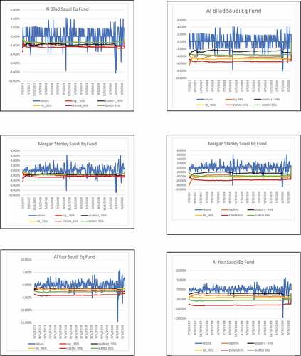
Tables 7 and 8 present the results of the parametric and non-parametric model performance in the conditional test, in addition to the quadratic loss and unexpected loss estimate measures at the 95% and 99% confidence levels.

Table 7. VaR performance under Quadratic Loss and Unexpected Loss functions at a 95% confidence level

	student t			log
	FR	QL	ULF	FR	QL	ULF
mf1	4.71%	8.311%	-0.141%	4.71%	12.465%	-0.196%
mf2	4.71%	7.618%	-0.115%	4.04%	11.772%	-0.174%
mf3	5.72%	7.966%	-0.141%	4.04%	11.427%	-0.177%
mf4	5.39%	7.616%	-0.114%	4.71%	11.423%	-0.145%
mf5	4.38%	8.310%	-0.123%	4.04%	12.117%	-0.158%
mf6	5.05%	9.694%	-0.139%	4.38%	14.540%	-0.189%
mf7	5.05%	9.348%	-0.151%	5.05%	12.463%	-0.162%
mf8	4.71%	9.220%	-0.135%	3.70%	12.29%	-0.17%
mf9	5.05%	5.885%	-0.106%	4.71%	10.385%	-0.153%
mf10	3.70%	8.312%	-0.140%	3.37%	13.157%	-0.184%
mf11	4.04%	7.274%	-0.119%	3.37%	12.120%	-0.188%
mf12	3.70%	4.504%	-0.097%	3.37%	14.541%	-0.185%
mf13	3.70%	7.623%	-0.160%	3.37%	11.430%	-0.193%
mf14	2.69%	3.471%	-0.103%	2.69%	11.777%	-0.175%
mf15	4.04%	7.620%	-0.145%	3.37%	10.736%	-0.185%
mf16	4.38%	6.235%	-0.126%	3.70%	8.659%	-0.168%
mf17	4.38%	8.311%	-0.128%	3.70%	12.464%	-0.183%
mf18	5.39%	7.617%	-0.105%	3.70%	11.771%	-0.159%
mf19	6.06%	7.618%	-0.128%	5.05%	13.156%	-0.186%
mf20	5.39%	10.038%	-0.113%	4.38%	12.807%	-0.157%
mf21	4.71%	9.349%	-0.129%	3.70%	11.773%	-0.187%
mf22	5.39%	7.273%	-0.126%	3.70%	13.158%	-0.193%
mf23	3.70%	8.308%	-0.101%	3.37%	14.191%	-0.143%
mf24	5.39%	4.500%	-0.067%	4.38%	10.038%	-0.121%
mf25	3.03%	6.932%	-0.142%	2.69%	4.854%	-0.132%
mf26	5.39%	7.965%	-0.128%	4.04%	12.118%	-0.176%

1. Bold values denote that the model has passed the conditional coverage test (Christofferson, 1998) at a 5% significance level 2. Bold and highlighted marks the lowest

Quadratic Loss (QL) (Lopez, 1999) across the VaR estimates. 3. Bold and underlined represents the lowest Unexpected Loss (UL) (Lee and Su, 2015) across the VaR estimates.

4. FR- represents the proportion of the failure rate or the binary loss function.

Table 8. VaR performance under quadratic loss and unexpected loss functions at the 99% confidence level

	Student t			log			EWMA			GARCH			HS
	FR	QL	UL	FR	QL	UL	FR	QL	UL	FR	QL	UL	FR	QL	UL
mf1	1.68%	2.425%	−0.056%	2.02%	7.273%	−0.126%	1.01%	1.040%	−0.037%	1.01%	2.079%	−0.045%	1.010%	2.080%	−0.064%
mf2	1.68%	2.079%	−0.050%	1.68%	7.617%	−0.110%	0.34%	0.693%	−0.022%	0.67%	1.732%	−0.041%	1.010%	2.079%	−0.059%
mf3	1.35%	2.079%	−0.054%	1.68%	5.888%	−0.115%	0.67%	0.694%	−0.032%	0.67%	1.734%	−0.057%	0.673%	2.427%	−0.074%
mf4	1.35%	1.385%	−0.030%	1.35%	6.577%	−0.080%	0.67%	1.039%	−0.022%	1.01%	2.770%	−0.049%	1.010%	3.116%	−0.053%
mf5	1.35%	1.732%	−0.045%	1.68%	5.541%	−0.096%	0.67%	1.386%	−0.037%	1.35%	2.426%	−0.062%	1.010%	1.3864%	−0.045%
mf6	1.35%	2.078%	−0.052%	1.35%	7.271%	−0.112%	1.01%	1.385%	−0.032%	1.35%	2.425%	−0.060%	1.010%	1.3853%	−0.0386%
mf7	1.68%	2.423%	−0.041%	2.36%	5.194%	−0.110%	1.01%	1.385%	−0.025%	1.35%	3.116%	−0.063%	1.010%	2.424%	−0.053%
mf8	1.68%	2.391%	−0.056%	2.02%	6.489%	−0.111%	1.01%	1.025%	−0.031%	1.01%	2.392%	−0.062%	1.010%	2.392%	−0.064%
mf9	1.68%	2.772%	−0.056%	2.36%	7.273%	−0.118%	1.35%	1.040%	−0.033%	1.35%	2.080%	−0.061%	1.010%	2.081%	−0.070%
mf10	1.35%	2.772%	−0.056%	1.68%	7.273%	−0.118%	0.34%	1.040%	−0.033%	1.01%	2.080%	−0.061%	1.347%	2.081%	−0.070%
mf11	1.01%	2.772%	−0.067%	1.68%	8.657%	−0.129%	0.67%	1.040%	−0.031%	1.01%	1.042%	−0.053%	1.347%	2.428%	−0.078%
mf12	1.68%	4.156%	−0.080%	2.02%	9.003%	−0.134%	0.67%	0.693%	−0.025%	0.67%	1.733%	−0.042%	1.347%	1.733%	−0.054%
mf13	1.35%	2.081%	−0.073%	1.35%	6.237%	−0.133%	0.67%	0.694%	−0.039%	1.01%	1.389%	−0.067%	0.673%	1.389%	−0.073%
mf14	0.67%	3.468%	−0.078%	1.35%	9.007%	−0.133%	0.34%	0.349%	−0.034%	0.67%	0.697%	−0.051%	2.357%	2.086%	−0.089%
mf15	1.68%	2.772%	−0.064%	1.68%	6.927%	−0.127%	0.67%	0.694%	−0.032%	0.67%	1.734%	−0.057%	1.010%	2.081%	−0.068%
mf16	1.35%	2.426%	−0.069%	2.36%	6.581%	−0.128%	0.67%	1.039%	−0.027%	1.01%	1.387%	−0.052%	1.010%	1.387%	−0.056%
mf17	1.68%	2.425%	−0.053%	2.02%	7.618%	−0.114%	0.34%	0.694%	−0.024%	0.67%	1.733%	−0.047%	1.010%	2.080%	−0.061%
mf18	1.68%	2.425%	−0.048%	1.68%	7.271%	−0.100%	0.34%	0.694%	−0.026%	1.01%	1.733%	−0.049%	1.010%	1.733%	−0.051%
mf19	1.68%	3.117%	−0.050%	2.36%	7.963%	−0.122%	0.67%	0.693%	−0.027%	0.67%	1.733%	−0.045%	1.684%	3.118%	−0.066%
mf20	1.35%	1.731%	−0.032%	2.02%	5.885%	−0.086%	0.34%	1.039%	−0.021%	1.01%	3.116%	−0.051%	1.010%	3.116%	−0.052%
mf21	1.35%	2.426%	−0.054%	2.02%	7.619%	−0.117%	0.34%	0.694%	−0.023%	0.67%	1.041%	−0.039%	1.010%	2.081%	−0.068%
mf22	1.35%	2.080%	−0.058%	1.68%	8.311%	−0.126%	0.34%	0.348%	−0.023%	0.67%	1.041%	−0.040%	1.010%	1.735%	−0.063%
mf23	1.01%	1.385%	−0.030%	2.02%	4.501%	−0.075%	0.67%	1.039%	−0.024%	1.01%	2.424%	−0.050%	2.020%	2.770%	−0.061%
mf24	1.68%	2.423%	−0.031%	2.02%	5.539%	−0.077%	0.34%	0.693%	−0.018%	1.01%	2.077%	−0.034%	1.010%	3.116%	−0.047%
mf25	0.67%	1.042%	−0.056%	1.01%	3.122%	−0.096%	0.67%	1.043%	−0.059%	0.67%	2.776%	−0.103%	1.010%	4.507%	−0.119%
mf26	1.68%	2.425%	−0.051%	2.36%	6.234%	−0.114%	0.34%	0.694%	−0.025%	0.67%	2.425%	−0.050%	0.673%	2.426%	−0.060%

1. Bold values denote that the model has passed the conditional coverage test at the 5% significance level 2. Bold and highlighted marks the lowest Quadratic Loss (QL) across the VaR estimates. 3. Bold and underlined represents the lowest Unexpected Loss (UL) across the VaR estimates. 4. FR- represents the proportion of the failure rate.

It is evidenced from the results in Table 7 that at the 95% confidence level, student-t (7) and HS (7) have recorded the best performance with the highest number of acceptances generated in the conditional test. At the 95% confidence level, the performance of the aforementioned models is much higher than the sophisticated models of EWMA and GARCH (1,1). None of the results for the EWMA and only 3 VaR estimates given by GARCH (1,1) passed the conditional tests at 95%. It is noteworthy that the conditional test does not account for the magnitude of loss, hence the conclusions from the QL and ULF for a long-term position are more meaningful as it overcomes the limitations. EWMA recorded the lowest QL and ULF for all of the funds and across the VaR estimates, confirming that the EWMA method provides a better VaR predicting performance than any other model for the given sample. The overall average quadratic loss and unexpected loss function of EWMA is the lowest across the VaR estimates followed by student-t distribution.

It is evidenced from the results in Table 8 that at the 99% confidence level, the EWMA approach has recorded the highest number of acceptances (12) in the conditional test, and it has thus outperformed all of the other VaR estimate measures. The lowest number of acceptances are seen in the conditional test for student-t (1), log (2), GARCH (1,1) (0) and HS (0). EWMA recorded the lowest QL and ULF for all of the funds and across the VaR estimates, confirming that the EWMA method at the 99% confidence level provides better VaR predicting performance than any other model for the given sample. The overall average quadratic loss and unexpected loss function of EWMA is the lowest across the VaR estimates, followed by GARCH (1,1).

From the graphical demonstration in Figure 1 and the aforementioned results discussed as shown in Tables 7 and 8, it can be inferred that at the 95% significance level, student—t distribution and EWMA at the 99% level have recorded the highest number of acceptances by passing the conditional test. EWMA showed the best performance with the highest number of acceptances in the conditional test and the lowest QL and ULF values for the 99% confidence level. Overwhelmingly for the given sample, irrespective of the confidence level, EWMA has been able to best capture the VaR of the maximum number of funds with the lowest magnitude of losses as measured by QL and ULF. The supremacy of EWMA has also been evidenced by DeGennaro and Richard (1990), Bollerslev et al. (1992), and Dowd (2005).

5. Limitations & directions for future research

Advancement in techniques and methods witnessed in studying the volatility of returns has been numerous. The present study has just applied selected VaR methods such as the GARCH (1,1) and EWMA methods to capture the downside risk potential of returns for a limited time period. The study can be extended to include the extended and robust VaR measures from the GARCH family, Montecarlo Simulation, Expected Value theory, Prospect ratio (Watanabe, 2007) to calculate the return per unit of downside risk, Lower Partial Moments (Bawa, 1975; Jean, 1975), Sortino and Van der Meer (1991) ratio based on the Minimum Acceptable Return as the point of exclusion, Omega ratio (Keating & Shadwick, 2002), Kappa ratio (Kaplan & Knowles, 2004) to measure the excess return adjusted for downside risk. It must be noted that the criteria set to measure the downside risk are sensitive to segregations and can sometimes generate distorted results.

6. Conclusion

In this paper, the novel risk management concept of Value-at-Risk (VaR), which has been embraced as one of the best tools in the financial literature to measure downside risk on mutual fund returns, has been examined in relation to the equity mutual funds. VaR has been estimated based on a selected set of parametric and non-parametric methods. These estimates were further examined for adequacy and accuracy using the conditional coverage backtesting procedure, quadratic loss function and unexpected loss function. The primary findings of this research paper confirm the observations that the financial return series of mutual funds listed on the Saudi Stock Market are leptokurtic with a large kurtosis, signifying that the variations in the net asset value of funds have more frequent occurrences and heavy tails than is estimated by the normal distribution. The outcome is that under the assumption of normal distribution, fund risk is understated. Therefore, considering a logistic distribution model of return is a better fit for analyzing the financial returns involved. The weekly predictive power of the traditional VaR models (student-t distribution, log distribution, historical simulation) and sophisticated volatility models (EWMA, GARCH (1,1)) were compared. Conventional methods tend to overestimate the VaR at both confidence levels and they show better unconditional coverage when compared to the sophisticated methods. The student-t distribution, log-normal and historical simulation methods qualify the unconditional coverage test and provide better results at the 5% level compared to the other models. However, the superiority of the lognormal and historical simulations vanish when the conditional coverage test is applied. The student-t-distribution provides the best estimate of VaR at the 5% level whereas EWMA is the best at the 1% level under the conditional coverage tests. The combined results of the proportion of failure rate, quadratic loss function and the unexpected loss function demonstrate that EWMA provides the best forecast of volatility compared to GARCH (1,1) in addition to the student-t- distribution, log-normal and historical simulations at both the 95% and 99% significance levels. The EWMA model has been found to be superior in terms of forecasting the volatility of returns compared to GARCH (1,1), especially for short-term horizons. The volatility weighted VaR approaches are able to capture the downside risk better than traditional methods at the 1% level. It is worth noting that this study has put forward strong evidence that volatility clustering can be effectively modeled using EWMA. No single measure can explain the mechanisms involved in the volatility of return in financial instruments, but the best VaR approach can be used as a risk management tool to minimize the downside risk losses of investments. Hence, a hybrid approach of both traditional and volatility models would be beneficial for the Saudi mutual fund sector rather than any single best VaR measure.

Acknowledgements

The author would like to thank the Deanship of Graduate Studies and Scientific Research, Dar Al-Uloom University, Riyadh, Saudi Arabia, for funding the research work.

Disclosure statement

No potential conflict of interest was reported by the author.

Additional information

Funding

This work was supported by the Deanship of Graduate Studies and Scientific Research, Dar Al-Uloom University, Riyadh, Saudi Arabia

Notes on contributors

Sunitha Kumaran

Risk can deceive even the most experienced investor. Intensive work on modelling or capturing risk has been the area mostly researched by the author. Risks that are not captured or considered in the portfolio management process will lead to future issues and reduce profits, hence it is critical to capture risk at ease. The current study has been an attempt to capture the downside risk and suggest a best method to quantity the same. The outcomes of the paper can enable investors to customize the risk estimation and set the tolerance level for the investment while setting optimal portfolio. VaR estimates are at present the most favored tool to capture unacceptable risk, but advancement in financial econometrics has been offering advanced and robust tools to model risk. Knowing more about the downside risk is crucial to the advancement of risk management techniques and avoiding future financial crisis.

Appendix 1

List of mutual funds

Table

mf1	Riyad Saudi Equity Fund	mf16	SEDCO Cap Flexi Saudi Equity Fund
mf2	Aljazaria Cap Saudi Equity Fund	mf17	Al Rajhi Saudi Equity fund
mf3	HSBC Saudi Equity Fund	mf18	Saudi (AUDI) opportunity Equity Fund
mf4	Al Arabi Saudi Equity Fund	mf19	Falcom Saudi Equity Fund
mf5	Al Muhasem Saudi Equity Fund	mf20	AlAhli Free Style Saudi Equity Fund
mf6	Al Rajhi Materials Sec Equity fund	mf21	SAIB Saudi Equity Fund
mf7	Albilad Pure Saudi Equity Fund	mf22	AlYusr Saudi Equity Fund
mf8	Morgan Stan Saudi Equity Fund	mf23	Saudi Isthithmar (SAUDI FRANSI) Saudi Equity fund
mf9	Alkhair Capital Saudi Equity Fund	mf24	Wasatah Saudi Equity fund
mf10	KSB Free Style Saudi Equity Fund	mf25	Jadwa Saudi Equity Fund—Class B
mf11	Dereyah Free Style Saudi Equity Fund	mf26	Osool Saudi Equity Tr Fund
mf14	Al nefale Comp Equity fund
mf15	BLOM Saudi Equity fund

References

- Abad, P., Benito, S., & López, C. (2014). A comprehensive review of value at risk methodologies. The Spanish Review of Financial Economics, 12(1), 15–32. https://doi.org/10.1016/j.srfe.2013.06.001
- Abad, P., & Benito, S. (2013). A detailed comparison of value at risk in international stock exchanges. Mathematics and Computers in Simulation, 94, 258–276. https://doi.org/10.1016/j.matcom.2012.05.011
- Aloui, C., Abaoub, E., & Bellalah, M. (2005). Long range dependence on Tunisian stock market volatility. International Journal of Business, 10 (4), 1–26. https://www.semanticscholar.org/paper
- Angelidis, T., Benos, A., & Degiannakis, S. A. (2007). A robust VaR model under different time periods and weighting schemes. Review of Quantitative Finance and Accounting, 28(2), 187–201. https://doi.org/10.1007/s11156-006-0010-y
- Ashley, R., & Randal, V. (2009). Frequency dependence in regression model coefficients: An alternative approach for modeling nonlinear dynamic relationships in time series. Econometric Reviews, 28(1–3), 4–20. https://doi.org/10.1080/07474930802387753
- Bali, T., & Theodossiou, P. (2007). A conditional-SGT-VaR approach with alternative GARCH models. Annals of Operations Research, 151(1), 241–267. https://doi.org/10.1007/s10479-006-0118-4
- Bawa, V. S. (1975). Optimal rules for ordering uncertain prospects. Journal of Financial Economics, 2(1), 95–121. https://doi.org/10.1016/0304-405X(75)90025-2
- Billio, M., & Pelizzon, L. (2000). Value-at-risk: A multivariate switching regime approach. Journal of Empirical Finance, 7(5), 531–554. https://doi.org/10.1016/S0927-5398(00)00022-0
- Black, F. (1976). Studies of stock price volatility changes. In: Proceedings of the 1976 Meeting of the Business and Economic Statistics Section, American Statistical Association Washington, D.C., pp. 171–181.
- Bollerslev, T., Chou, R. Y., & Kroner, K. P. (1992). ARCH modeling in finance: A review of the theory and empirical evidence. Journal of Econometrics, 52 (1–2), 5–59. https://doi.org/10.1016/0304-4076(92)90064-X.
- Bollerslev, T. (1986). Generalized Autoregressive Conditional Heteroskedasticity. Journal of Econometrics, 31(3), 307–327. https://doi.org/10.1016/0304-4076(86)90063-1
- Bollerslev, T. (1987). A conditionally heteroskedastic time series model for speculative prices and rates of return. Review of Economics and Statistics, 69(3), 542–547. https://doi.org/10.2307/1925546
- Boudoukh, J., Richardson, M., & Whitelaw, R. F. (1997). The best of both worlds: A hybrid approach to calculating value at risk. SSRN Electronic Journal. https://doi.org/10.2139/ssrn.51420
- Christoffersen, P. (1998). Evaluating interval forecasting. International Economic Review, 39(4), 841–862. https://doi.org/10.2307/2527341
- Curto, J. D., Pinto, J., & Tavares, G. (2009). Modeling stock markets volatility using GARCH models with Normal, Student-t and stable Paretian distributions. Statistical Papers, 50(2), 311–321. https://doi.org/10.1007/s00362-007-0080-5
- Danielsson, & De Vries. (2000). Value-at-risk and extreme returns. Annales d’Économie et de Statistique, 60(60), 239–270. https://doi.org/10.2307/20076262
- DeGennaro, R. P., & Richard, B. (1990). Stock returns and volatility. Journal of Financial & Quantitative Analysis, 25 (2), 203–214. https://ssrn.com/371920
- Ding, Z., Granger, C. W., & Engle, R. F. (1993). A long memory property of stock market returns and a new model. Journal of Empirical Finance, 1(1), 83–106. https://doi.org/10.1016/0927-5398(93)90006-D
- Dowd, K. (2005). Measuring Market Risk (2nd ed.). John Wiley & Sons Inc.
- Emenogu, N. G., Adenomon, M. O., & Nweze, N. O. (2020). On the volatility of daily stock returns of total Nigeria Plc: Evidence from GARCH models, value-at- risk and backtesting. Financial Innovation, 6(18). https://doi.org/10.1186/s40854-020-00178-1
- Engle, R. F. (1982). Autoregressive Conditional Heteroskedasticity with estimates of the variance of United Kingdom inflation. Econometrica, 50 (4), 987–1007. https://doi.org/10.2307/1912773 JSTOR 1912773
- Fama, E. (1965). The behaviour of stock-market prices The. Journal of Business, 38 (1), 34–105. https://doi.org/10.1086/294743.
- Feunou, B., Mohammad, R. J.-P., & Tedongap, R. (2013). Modeling market downside volatility. Review of Finance, 17(1), 443–481. https://doi.org/10.1093/rof/rfr024
- Goorbergh, R. V., & Vlaar, P. J. (1999). DNB Staff Reports (discontinued) (Netherlands Central Bank). https://www.dnb.nl/binaries/sr040_tcm46-146818.pdf
- Grzegorz, M. (2013). Parametric or Non-parametric estimation of value-at-risk. International Journal of Business and Management, 8(11). https://doi.org/10.5539/ijbm.v8n11p103
- Guha Deb, S. (2017). A VaR-based downside risk analysis of Indian Equity mutual funds in the pre and post-global financial crisis periods. Journal of Emerging Market Finance, 18(2), 210–236. https://doi.org/10.1177/0972652719846348
- Hansen, P. R., & Lunde, A. (2005). A forecast comparison of volatility models: Does anything beat a GARCH(1,1). Journal of Applied Econometrics, 20(7), 873–889. https://doi.org/10.1002/jae.800
- Herzberg, M., & Sibbertsen, P. (2004). Pricing of options under different volatility models. Technical Report/ Universit¨at Dortmund, SFB 475, Komplexit¨atsreduktion in Multivariaten Datenstrukturen, 62. https://www.econstor.eu/bitstream/10419/22575/1/tr62-04.pdf
- Jean, W. H. (1975). Comparison of moment and stochastic dominance ranking methods. The Journal of Financial and Quantitative Analysis, 10(1), 151–161. https://doi.org/10.2307/2330323
- Jorion, P. (2007). Value at risk: The new benchmark to measure financial risk (3rd ed.). McGraw- Hill.
- Kaplan, P. D., & Knowles, J. A. (2004). Kappa: A generalized downside risk-adjusted performance measure [Working Paper]. Miscellaneous publication, Morningstar Associates and York Hedge Fund Strategies.
- Keating, C., & Shadwick, W. F. (2002). A universal performance measure. Journal of Performance Measurement, 6(3), 59–84. https://www.actuaries.org.uk/system/files/documents/pdf/keating.pdf
- Kheir, I. (2019). GARCH modeling of value at risk and expected shortfall using bayesian model averaging (CUNY Academic Works, City University of New York).https://academicworks.cuny.edu/hc_sas_etds/510
- Korkmaz, T., & Aydın, K. (2002). Using EWMA and GARCH methods in VaR calculations: Application of ISE-30 Index. The International Conference in Economics, Ankara, Turkey. https://content.csbs.utah.edu/~ehrbar/erc2002/pdf/P161.pdf
- Kupiec, P. (1995). Techniques for verifying the accuracy of risk measurement models. The Journal of Derivatives, 3(2), 73–84. https://doi.org/10.3905/jod.1995.407942
- Lee, C.-F., & Su, J.-B. (2015). Value-at-Risk estimation via a semi-parametric approach: Evidence from the stock markets. In C.-F. Lee & J. Lee (Eds.), Handbook of Financial Econometrics and Statistics (pp. 1399–1429). Springer Science & Business Media. https://doi.org/10.1007/978-1-4614-7750-1_51
- Lee, T. H., & Saltoglu, B. (2002). Assessing the risk forecasts for Japanese stock market. Japan and the World Economy, 14 (1), 63–85. https://doi.org/10.1016/S0922-1425(01)00080-9.
- Lin, C., & Shen, S. (2006). Can the student-t distribution provide accurate value at risk? The Journal of Risk Finance, 7(3), 292–300. https://doi.org/10.1108/15265940610664960
- Liu, H.-C., & Hung, J.-C. (2010). Forecasting volatility and capturing downside risk of the Taiwanese futures markets under the financial tsunami. Managerial Finance, 36(10), 860–875. https://doi.org/10.1108/03074351011070233
- Lopez, J. A. (1999). Methods for evaluating value-at-risk estimates. Federal Reserve Bank of San Francisco Economic Review, 2, 3–17. https://www.newyorkfed.org/medialibrary/media/research/staff_reports/research_papers/9802.pdf
- Mandelbrot, B. (1963). The Variation of certain speculative prices. The Journal of Business, 36 (4), 394. https://doi.org/10.1086/294632.
- Markowitz, H. (1959). Portfolio Selection Efficient Diversification of Investment. John Wiley & Sons, Inc.
- Mills, T. (1965). Modelling skewness and kurtosis in the London stock exchange FT-SE index return distributions. Journal of the Royal Statistical Society Series D (The Statistician), 44(3), 323–332. https://doi.org/10.2307/2348703
- Morgan Bank, J. P. (1996). Risk metrics—Technical document (4th ed.).
- Raza, H., Arshad, H., & Rashid, A. (2019). The impact of downside risk on expected return:evidence from emerging economies. The Lahore Journal of Business, 8(1), 91–106. https://doi.org/10.35536/ljb.2019.v8.i1.a5
- Roy, A. D. (1952). Safety First and the Holding of Assets. Econometrica, 20(3), 431–449. https://doi.org/10.2307/1907413
- Sinha, T., & Chamu, F. (2000). Comparing different methods of calculating value-at-risk. SSRN: Electronic Journal. https://doi.org/10.2139/ssrn.706582
- Skrinjaric, T. (2014). Investment strategy on the Zagreb stock exchange based on Dynamic DEA. Croatian Economic Survey, 16(1), 129–160. https://doi.org/10.15179/ces.16.1.5
- Sortino, F. A., & Van der Meer, R. (1991). Downside risk. Journal of Portfolio Management, 17(4), 27–31. https://doi.org/10.3905/jpm.1991.409343
- Su, J.-B., & Hung, J.-C. (2018). The value-at-risk estimate of stock and currency-stock portfolios’ returns. MDPI-Risk, 6(133). https://doi.org/10.3390/risks6040133>
- Tusji, C. (2016). Does the fear gauge predict downside risk more accurately than econometric models? Evidence from the US stock market. Cogent Economics & Finance, 4(1). https://doi.org/10.1080/23322039.2016.1220711
- Watanabe, Y. (2007). Is Sharpe ratio still effective? The Journal of Performance Measurement, 11(1), 55–66. https://spauldinggrp.com/product/sharpe-ratio-still-effective/
- Zoran, J., & Ivica, T. (2014). Empirical estimation and comparison of normal and student-t linear VaR on the Belgrade stock exchange. SINTEZA 2014: The use of the internet and development perspectives (Singidunum University , Belgrade) (pp. 298–302). https://doi.org/10.15308/sinteza-2014-298-302