Convexity arbitrage – the idea which does not work

Abstract

Algorithmic trading, so popular nowadays, uses many strategies that are algorithmizable and promise profitability. This research answers the question whether it is possible to successfully use a convexity arbitrage strategy in a bond portfolio in financial practice. It should provide a positive expected excess return and a small or zero potential loss. Convexity arbitrage has been described in academic literature before, but an assessment of its practical success is lacking. Arbitrage portfolio, which consists of two portfolios of bonds, is constructed theoretically and practically. These two portfolios have the same Macaulay Duration and price, but a different convexity at a certain yield to maturity point (YTM point). As the first portfolio is long, while shorting the second (with higher convexity), the result would therefore be a market-directional bet on parallel YTM shifts of the same size. Methodology: a mathematical definition of this arbitrage; the construction of the arbitrage portfolio; back-testing on USD and EUR zero-coupon yield curve. To construct the arbitrage portfolio could be unrealistic on markets with low liquidity. Moreover, the assumption of parallel YTM shifts of the same size is not fulfilled enough to ensure that the arbitrage is profitable. This research helps practitioners considering the implementation of this strategy in algorithmic trading to make an adequate assessment. Its findings show that the practical and profitable utilization of convexity arbitrage is unrealizable.

Keywords:

• convexity arbitrage
• algorithmic trading
• YTM shift
• convexity

PUBLIC INTEREST STATEMENT

Algorithmic trading is very popular today. This is an approach where investment or speculative decisions are not made based on an intuitive decision but based on an algorithm that analyzes historical and current market data. Many investors believe that the algorithmic implementation of some procedures provides the possibility of making speculative profit at little or no risk. Statistical arbitrage, which often evokes such a feeling, also penetrates such ideas. However, the situation is not so simple. The article analyses one of the statistical arbitrages, also known as convexity arbitrage, and shows that the notion of making a profit at little or no risk is wrong.

1. Introduction

Convexity arbitrage in bond portfolios has been mentioned in financial literature before (Questa (1999)), but an assessment of its practical implementation and the possible practical success of this speculative technique is lacking.

The main contribution of this research is to answer the question whether convexity arbitrage is suitable for financial practice.

Convexity arbitrage is performed using a portfolio that is adequate for this type of arbitrage—arbitrage portfolio. The arbitrage portfolio consists of two portfolios of bonds with the same Macaulay Durations and prices, but with different convexities at a certain yield to maturity (YTM) point. Let’s mark this YTM point as a point of contact where the curves of price with respect to YTM for both portfolios touch here. As portfolio 1 (portfolio with higher convexity) is long when portfolio 2 is short, one portfolio should always outperform the other one whenever there is a change of YTM from the point of contact. It is assumed that the YTM change has the same direction and size for both portfolios. Detailed theoretical analysis of this arbitrage is in chapter 3. In this research we try to construct (theoretically and also practically) an arbitrage portfolio, and, moreover, we back-test this speculative approach using a real liquid financial market—the evolution of USD and EUR interest rate zero-coupon curve. This back-testing is necessary to assess whether the preconditions necessary for successful functionality are practically fulfilled enough to ensure that convexity arbitrage is a profitable strategy for financial practice. To clarify the aim of the study we explicitly formulate two hypotheses; Hypothesis 1: It is possible practically to construct an arbitrage portfolio. Hypothesis 2: A convexity arbitrage strategy, using an arbitrage portfolio, always provides positive payoffs in financial practice.

This research is typical one of financial engineering.¹ We also provide certain examples in the text in order to explain the strategy better to financial practitioners and to show its difference from risk management techniques (Janda and Kourilek, 2020).

Convexity arbitrage is a type of statistical arbitrage. Statistical arbitrage, in our point of view, should be defined as the arbitrage between two prices (interest rate sensitive) where the first price is a market price and the second one is a certain price that we expect in the future based on certain statistical calculations. It provides a positive expected excess return and an acceptably small potential loss.

In the literature review we shall return to the development of the statistical arbitrage concept.

2. Literature review

The concept of arbitrage is one of the fundamentals in financial literature and has been used before in the classical analysis of market efficiency (Fama (1969), Ross (1976)), according to which arbitrage opportunities were quickly exploited by speculators. The basic division of arbitrage is into “pure” and “statistical”. However, pure arbitrage opportunities (defined as profit-taking using two different market prices of an asset at one time) are unlikely to exist in a real-life throughout trading environment (Shleifer and Vishny (1997), Alsayed and McGroarty (2014)). The possible success of statistical arbitrage in practical finance is still under discussion.

It is commonly accepted that statistical (not pure) arbitrage started in the mid-1980s when Nunzio Tartaglia assembled a team of quantitative analysts at Morgan Stanley to uncover statistical mispricing on equity markets (Gatev et al. (2006)). While the definition of pure arbitrage is clear, the definition of statistical arbitrage is more complicated. The common definition of statistical arbitrage as a zero-cost trading strategy with a positive expected payoff and no possibility of a loss is acceptable for pure arbitrage, but it is too strict for statistical arbitrage. The term “zero-cost strategy” means a trading or financial decision that costs nothing to implement. Connor and Lasarte (2003) use the probability of certain loss in their definition of statistical arbitrage as a zero-cost portfolio where the probability of a loss is very small but not exactly zero, or, in other words, a statistical arbitrage strategy is a relative value strategy with a positive expected excess return and an acceptably small potential loss. Hogan et al. (2004) provide an alternative definition of statistical arbitrage that focuses on long-horizon trading opportunities. Hogan’s statistical arbitrage is a long-horizon trading opportunity that, at the limit, generates a risk-free profit. According to this definition, statistical arbitrage satisfies four conditions:

1. It is a zero-cost, self-financing strategy.

2. It has, at the limit, a positive expected discounted payoff.

3. The probability of a loss converges to zero.

4. The time-average variance converges to zero if the probability of a loss does not become zero in a finite time.

The fourth condition is applied only when there exists a positive probability of losing money.

According to Saks and Maringer (2009), statistical arbitrage accepts negative payoffs as long as the expected positive payoffs are high enough and the probability of losses is small enough. Stefanini (2006) uses the expected value while stating that statistical arbitrage seeks to capture imbalances in the expected value of financial instruments while trying to be market neutral. Focardi et al. (2016) focus on uncorrelated returns, reporting that statistical arbitrage strategies aim to produce positive, low-volatility returns that are uncorrelated with market returns.

All the definitions mentioned above use profit/loss assessment, but the strategies themselves could be based on different principles. In the case of pair trading (one of the most popular strategies), we perform a simultaneous opening of the long and short positions in each of two assets (portfolios) and utilize the mean reversion behavior of the ratio of the prices to achieve a profit (Gatarek et al. (2014), Alexander and Dimitriu (2005), and Nath (2006)). However, not all strategies need mean reversion; some need a persistently positive carry spread. Volatility arbitrage identifies relative value opportunities between volatilities. Swap spread plays a fixed spread against a floating spread; mortgage arbitrage models the spread of mortgage-backed securities compared to treasury bonds. Capital structure arbitrage profits from the spread between various instruments of the same company. If spreads are too narrow, these strategies are less profitable and can turn into a loss. In addition, not all strategies are zero-cost. Among other statistical arbitrages, we should mention term structure models utilizing the spread between yields or future prices.

Other important research in the area of statistical arbitrage was done by Pole (2007), Montana (2009), Burgess (2000), Avellaneda and Lee (2008), Thomaidis, Kondakis and Dounias (2006), Zapart (2003), and Hillier et al. (2006), Focardi et al. (2016), Cui et al. (2020), in the area of bond portfolio immunization by Ortobelli et al. (2018).

Technological developments in computational modelling have also facilitated the use of statistical arbitrage in high-frequency trading and the so-called machine learning methods, such as neural networks and genetic algorithms (Brogaard et al. (2014), Ortega and Khashanah (2014)). In more recent years, statistical arbitrage has attracted renewed interest in emerging areas such as bitcoin (Payne and Tresl (2015), Lintilhac and Tourin (2017)), big data (McAfee et al. (2012), Lazer et al. (2014), Chaboud et al. (2014), and Nardo et al. (2016)) and factor investing (Maeso and Martellini (2017)). Algorithmic trading is now responsible for more than 70% of the trading volume on the US markets (Hendershott et al. (2011), Nuti et al. (2011), and Birke and Pilz (2009)) used a non-arbitrage approach utilizing convexity for their contribution to the field of financial options. From our point of view, no more relevant literature specifically about convexity arbitrage is available (in WOS, Scopus or other scientific databases), apart from Questa (1999).

3. Methodology of empirical research

3.1. Theoretical background

Let us present an example of convexity arbitrage strategy implementation to explain its concept clearly. The goal is to create an arbitrage portfolio that consists of two portfolios of bonds with the same Macaulay Durations and price, but with different convexities at a certain YTM point. The arbitrage portfolio is sufficient for convexity arbitrage. As portfolio 1 is long when portfolio 2 is short, one portfolio should always outperform the other one whenever there is a same change in YTM from the point of contact of the price/YTM curve. YTM is defined in the equation (1)(1) $P={\left(1+\frac{d}{T}YTM\right)}^{-1}\left[c+\frac{c}{\left(1+YTM\right)}+\frac{c}{{\left(1+YTM\right)}^2}+\dots +\frac{c+100}{{\left(1+YTM\right)}^{n-1}}\right]$(1) .

(1) $P={\left(1+\frac{d}{T}YTM\right)}^{-1}\left[c+\frac{c}{\left(1+YTM\right)}+\frac{c}{{\left(1+YTM\right)}^2}+\dots +\frac{c+100}{{\left(1+YTM\right)}^{n-1}}\right]$(1)

where P is the dirty price of a bond in the percentage of its face value on purchasing day, c is the coupon rate per the coupon period, YTM is the yield to maturity per the coupon period, d is the number of days between the first coupon payment and the purchasing day, n is the number of coupon payments till the maturity and T is the number of days inside the coupon period.

An example of such a chart is in Figure 1, where the point of contact is at YTM = 3.5%. We assume the ideal case, where YTM develops for both portfolio 1 and portfolio 2 in the same way (shifts of the same value and direction). The Price/YTM chart of each of our two portfolios is in Figure 1.

Figure 1. P/YTM charts for a typical coupon bond (blue thick line) and a bond artificially created (red thin line) by theoretical construction. These two bonds form an arbitrage portfolio. “Price(crcy)” means price in a certain currency.

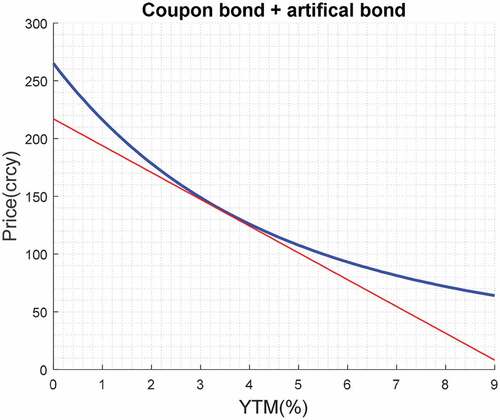
• Portfolio 1 (the blue thick line in Figure 1) is represented by one typical coupon bond with 30 years to maturity; fixed coupon = 5.5; face value = 100.

• Portfolio 2 (the red thin line in Figure 1) is represented by a theoretical (artificial) bond defined by the price formula: P(YTM) = −23.2 YTM+217.

YTM development (Figure 2-left, Figure 2-right) depicts two separate cases described by formula (2) and (3), where t is time.

(2) $YTM\hspace{0.17em}\left(t\right)=-\hspace{0.17em}t+3.5$(2)

(3) $YTM\hspace{0.17em}\left(t\right)=t+3.5$(3)

Figure 2. Possible development of YTM.

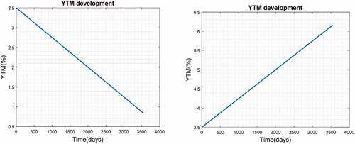
Initially, it moves from YTM = 3.5% downward (Figure 2-left), and then from this point upward (Figure 2-right)

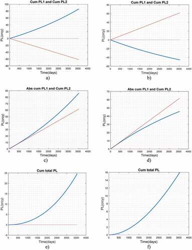
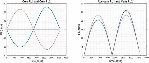
In Figure 3(a,c) we observe that in the case of a downside movement of YTM from 3.5% (according to Figure 2(a)), the profit that arises from portfolio 1 (blue thick line) is always higher than the loss on portfolio 2 (red thin line). In Figure 3(a) we observe the cumulative profit and loss on portfolio 1 and portfolio 2. In Figure 3(c) we see the absolute value of both cumulative profits. We use absolute values for better visual comparison. Finally, Figure 3(e) represents the sum of both cumulative P/L totals, which is of positive value. Analogically, if YTM moves from 3.5% upside (according to Figure 2(b)), the profit arising from portfolio 2 is always higher than the loss on portfolio 1. The subFigure 3(b,d,f) represent the cumulative profit/loss on portfolio 1 and portfolio 2 (3b), the absolute value of P/L (3d) for better comparison, and, finally, the cumulative P/L (3 f) of the whole strategy.

Figure 3. Cumulative P/L for portfolio 1 and for portfolio 2 in subfigures a), b); absolute value of cumulative P/L for portfolio 1 and for portfolio 2 in subfigures c), d); total cumulative P/L of both portfolios in subfigures e), f). Subfigures a), c), e) are for the case that YTM develops according to Figure 2-left, subfigures b), d), f) are for the case in Figure 2-right. “PL(crcy)” means PL in a certain currency.

Let us give another example, this time using the artificial YTM development that is given by formula (4) (Figure 4):

(4) $YTM\left(t\right)=sin\left(t\right)+3.5$(4)

Figure 4. Possible development of YTM.

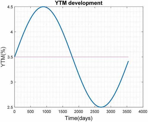
The YTM development starts from 0 on the vertical axis and continues to the right. The resulting cumulative P/L for each portfolio is in Figure 5-left, and the absolute value is in Figure 5-right.

Figure 5. Cumulative P/L on long portfolio 1(blue thick line) and short portfolio 2(red thin line) (left), cumulative P/L in absolute values (right). “PL(crcy)” means PL in a certain currency.

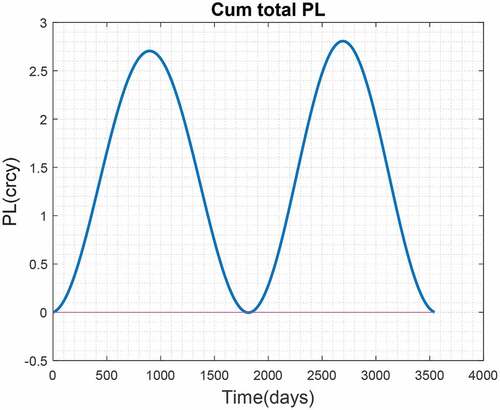
The resulting development of P/L for the whole strategy is in Figure 6.

Figure 6. Total cumulative P/L of a convexity arbitrage strategy. “PL(crcy)” means PL in a certain currency.

We may formulate assumptions necessary for the successful functionality of this strategy:

YTM performs shifts of the same size and direction for both portfolios. In this case, convexity arbitrage could be considered to be a risk-free and profitable strategy from which we may expect a positive pay-off and zero loss.

Then the expected P/L development could be characterized as follows

If the opening of long and short positions is done at the point of contact, and YTM keeps moving downward or upward, the cumulative P/L is always positive, irrespective of the direction. If YTM moves away from the contact point, the P/L increases. Analogically, if YTM moves toward the contact point, the P/L decreases.

The serious limitation of this strategy is that it may expose the investor to losses when there are nonparallel YTM shifts. Non-parallel shifts are quite common, and, in order to obtain a useful assessment, if the assumption of parallel YTM shifts mentioned above is fulfilled sufficiently to ensure that convexity arbitrage is a profitable strategy in practice, we have to perform certain quantitative back-testing.

3.2. Methodological steps

The methodology comprises the following steps:

1. A mathematical definition of convexity arbitrage conditions for realization.

2. Construction of an arbitrage portfolio that consists of two portfolios—portfolio 1 and portfolio 2 (theoretically and practically).

3. Back-testing on USD and EUR zero-coupon curve. Back-testing is implemented in a Matlab programming environment. In the research, we used information on zero-coupon curves in the period 1999–2018 (4900 working days) for USD zero-coupon rates, 2004–2018 (3500 working days) for EUR zero-coupon rates. We assume the bonds in portfolio to be CMT (Constant Maturity Time) bonds.

For both portfolios, we assume the same Macaulay Durations at the point of contact (equation 5(5) $DU{R}_1\left(YT{M}_A\right)=DU{R}_2\left(YT{M}_A\right)$(5) ).

(5) $DU{R}_1\left(YT{M}_A\right)=DU{R}_2\left(YT{M}_A\right)$(5)

where DUR₁(YTM_A) and DUR₂(YTM_A) are Macaulay Durations at point A. We now use the letter A to indicate the point of contact. General equation 6(6) $P_{\left(YTM\right)}^{\prime }=-DUR\left(YTM\right)\frac{P\left(YTM\right)}{1+YTM}$(6) implies that the values of the first derivative must be the same if the same prices are at the point of contact.

(6) $P_{\left(YTM\right)}^{\prime }=-DUR\left(YTM\right)\frac{P\left(YTM\right)}{1+YTM}$(6)

where P´(YTM) is the first derivative with respect to YTM, P(YTM) is the price of portfolio and DUR(YTM) is Macaulay Duration. The general equations describing the situation in the arbitrage portfolio can therefore be written as follows.

(7) $P_1\left(YT{M}_A\right)=P_2\left(YT{M}_A\right)$(7)

(8) ${P_1}^{\prime }\left(YT{M}_A\right)={P_2}^{\prime }\left(YT{M}_A\right)$(8)

(9) $conve{x}_{1\left(YT{M}_A\right)}>conve{x}_{2\left(YT{M}_A\right)}$(9)

where P₁ (YTM_A) is the price of portfolio 1 at point A; P₂ (YTM_A) is the price of portfolio 2 at point A, P´₁ (YTM_A) and P´₂ (YTM_A) are the first derivatives of prices of portfolio 1 and portfolio 2 at point A; convex₁ and convex₂ are values of the convexity of portfolio 1 and portfolio 2 at point A on the YTM axis.

4. Results

4.1. Construction of an arbitrage portfolio

The analytical solution of the set of equations (7-9)(7) $P_1\left(YT{M}_A\right)=P_2\left(YT{M}_A\right)$(7) deals with polynomial equations of order higher than 5 in the case of longer maturities, so we have to deal with numerical solutions. Solving analytically means finding an explicit equation without making approximations. When solving polynomial equations of higher order, analytic solutions can be difficult and sometimes impossible. And that’s why a numerical solution using the Matlab programming environment was used to find bond parameters for the creation of an arbitrage portfolio, while the requirements for bond parameters were such that bonds were commonly available on liquid bond markets. From the solutions, we choose one where the value of the point of contact equals approximately the mean of YTM, which results from the zero–coupon curve evolution in Figure 9 (for USD) and Figure 12 (for EUR), and we expect movements on both sides of this point:

Figure 7. P/YTM charts of two portfolios, the first of which consists of one zero-coupon bond (blue thick line) and the second of two zero-coupon bonds (red thin line). “Price(crcy)” means price in a certain currency.

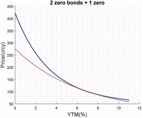
Figure 8. P/YTM charts of two portfolios, both of them consist of one zero-coupon bond. “Price(crcy)” means price in certain currency.

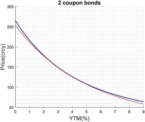
Figure 9. Daily shape changes of USD zero-coupon yield curve, period 1999–2018 (4900 working days), source: Reuters.

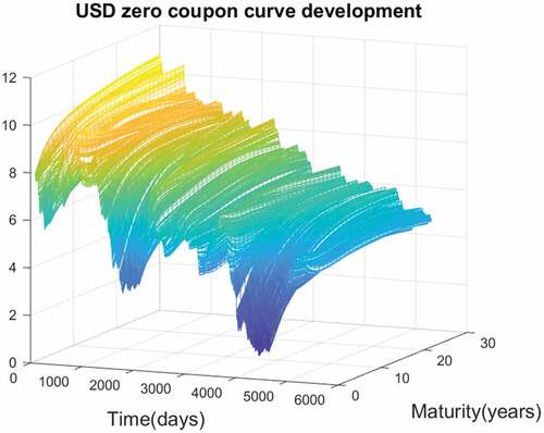
Figure 10. Cumulative P/L on long portfolio 1(blue thick line) and short portfolio 2 (red thin line), (left) and total cumulative P/L (right) during back-testing of convexity arbitrage strategy. “PL(crcy)” means PL in a certain currency.

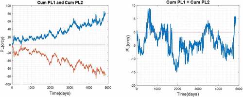
Figure 11. Schematic representation of the expected development of total cumulative P/L of portfolio 1 and portfolio 2 in case that convexity arbitrage works properly during back-testing. “PL(crcy)” means PL in a certain currency.

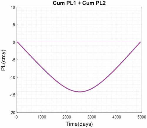
Figure 12. Daily shape changes of EUR zero-coupon yield curve, period 2004–2018 (3500 working days) source: Reuters.

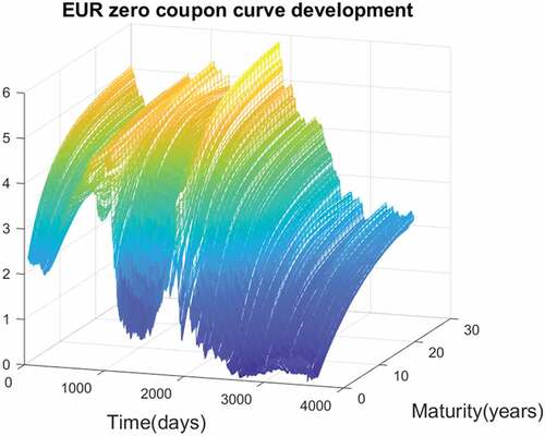
Figure 13. Cumulative P/L on long portfolio 1(blue thick line) and short portfolio 2 (left) and total cumulative P/L (right) during back-testing of convexity arbitrage strategy. “PL(crcy)” means PL in a certain currency.

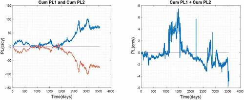
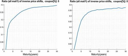
Figure 14. Ratio of number of inverse price shifts for bond with maturity = 1 year with respect to bonds with maturities of 1–30 years (fixed coupon rate bonds) for USD (left) and for EUR (right); the figures demonstrate that the presumption of parallel YTM shifts is empirically only partly fulfilled.

The solution used for back-testing the USD zero–coupon curve:

• Portfolio 1 is basically a portfolio of two zero–coupon bonds:

  • 1-year maturity zero bond, price at 7% = 51.72; face value = 55.34

  • 30-year maturity bond, price at 7% = 48.28; face value = 367.49

• Portfolio 2 is a zero-coupon bond: 15 years to maturity, price at 7% = 100; face value = 275.90.

The point of contact is at YTM = 7%, and the value of both portfolios at this point is 100. As shown in Figure 7, the portfolios are constructed in such a way as to have the same Macaulay Duration but a different convexity. Therefore, as portfolio 1 (the blue thick line in Figure 7) is long, while shorting the 15-year zero (the red thin line in Figure 7), the result should be a profitable strategy under the assumptions mentioned above. To back-test the EUR zero–coupon curve, we again choose a solution where the value of the point of contact) equals approximately the mean of YTM, which results from the zero–coupon curve evolution in Figure 12:

The portfolio consists of:

• Portfolio 1—represented by one typical coupon bond 1:30 years to maturity; fixed coupon = 5.5; face value = 100.

• Portfolio 2—represented by one typical coupon bond: 20 years to maturity; fixed coupon = 2.35; face value = 206.

The point of contact is at YTM = 3.5% and the price is the same for portfolio 1 and portfolio 2.

Analogically to the USD case, as portfolio 1 (the blue thick line in Figure 8) is long, while shorting the 20-year bond (the red thin line in Figure 8), the result should be a profitable strategy under the assumptions mentioned above.

4.2. Back-testing a USD zero–coupon curve

We use USD zero–coupon curve evolution (Figure 9) on a daily basis to calculate the change of price of portfolio 1 and portfolio 2. Figure 9, and also Figure 14, show how the shape of the curve changes from day to day. Depending on the shape of the curve, the price and YTM is calculated for each day, Fabozzi (2010). Using the changes in prices, we evaluate P/L using the strategy.

Based on the results of the back-testing displayed in Figure 10, where we observe the development of P/L using the convexity arbitrage strategy, we may conclude that this arbitrage does not work well because it does not provide expected P/L development for well-functioning strategy. Total cumulative P/L develops according to Figure 10-right during the back-testing. And if the strategy worked well, there would be an initial decrease in the total cumulative P/L below zero, and then a turnover at the contact point at which YTM = 7%, followed by a move upwards towards zero. This is because back-testing process begins at point 0, ends after 4900 days. During back-testing, we first move from higher YTMs to the contact point, and then from the contact point to lower YTM values. A detailed explanation of the expected back-testing results for a well-functioning strategy is described in the penultimate paragraph of chapter 3.1. The expected shape of P/L development during back-testing in this case is shown in Figure 11.

The contact point in our portfolio is 7%, which is the mean value of YTM (calculated on USD zero–coupon curves in Figure 9).

4.3. Back-testing a EUR zero–coupon curve

Analogically to the back-testing of the strategy on UDS zero–coupon curve, we back-tested the strategy on the EUR zero coupon curve. Based on the results in Figure 13, where we observe the development of P/L (portfolio 1-blue thick line, portfolio 2-red thin line in Figure 13-left, total cumulative P/L of the whole strategy in Figure 13-right), we may conclude that this arbitrage does not work on the EUR market either because the expected shape of the total cumulative P/L development in that case is also shown in Figure 11.

The explanation of this conclusion is analogical to the case in chapter 4.2.

4.4. Results of testing parallel YTM shifts of the same size

Arbitrage would work properly in the case of the same maturities of portfolios 1 and 2 in the arbitrage portfolio because in this case the shifts of YTM will be parallel and of the same size (Fabozzi (2010)). However, if the Macaulay Durations must be the same and the convexities must be different, portfolios 1 and 2 must have different term to maturity to set up the arbitrage portfolio. This claim can be proven using equations (7-9(7) $P_1\left(YT{M}_A\right)=P_2\left(YT{M}_A\right)$(7) ). In other words, it is possible to build an arbitrage portfolio that meet equations (7-9)(7) $P_1\left(YT{M}_A\right)=P_2\left(YT{M}_A\right)$(7) only with the help of portfolios 1 and 2 of the different bond maturities. Therefore, in order to generate a positive P/L and an acceptably small loss for different maturities the parallel YTM shifts must be ensured by changes of zero–coupon curve shape. However, based on a large empirical experience with the evolution of zero-coupon yield curves, it is impossible.

In order to confirm the results of the back-testing and to assess in more detail the practical validity of the assumptions for arbitrage functionality that we formulated at the end of chapter 3.1, we carried out tests of parallel YTM shifts and the size of YTM shifts for short and long maturities of bonds.

In approximately 25 % of USD zero–coupon curve shape change and in 35 % of EUR zero–coupon curve shape change we empirically observe inverse bond price shifts (it also means inverse YTM shifts) in the comparison of short-term bonds with long-term bonds (see, Figure 14 where we consider fixed coupon rate bonds). So, we empirically observe that the important assumption about the parallel YTM shifts is only partly fulfilled. But it also means that in approximately 65–75 % of cases the YTM shifts are almost parallel. It seems to be sufficient to ensure a positive payoff on average, but the other important presumption about the same magnitude of the YTM shifts is also only partly fulfilled. It results from the zero-coupon rates behavior in the Figures 9 and 12. The magnitude of the daily YTM shifts differs between long and short-term maturities.

5. Conclusions

In the context of convexity arbitrage strategy, we have to deal with more serious troubles.

The initial problem is to propose theoretically an arbitrage portfolio of liquid assets that fulfills equations (7-9)(7) $P_1\left(YT{M}_A\right)=P_2\left(YT{M}_A\right)$(7) , as we deal with a set of polynomial equalities of higher order. Moreover, its practical realization could be problematic mainly on illiquid markets because of difficulties in identifying the liquid issues. But these troubles can eventually be solved. We can conclude that hypothesis 1 is confirmed.

Convexity arbitrage has theoretical potential to work; however, from the results of back-testing the performance of this arbitrage, we conclude that this strategy did not work in the USD and EUR bond markets because the expected development of the P/L curve was not provided (chapter 4.2 and 4.3). This means that in the case of USD and EUR interest rates evolution, the important assumption of parallel YTM shifts, ideally of the same direction and size, was not sufficiently fulfilled to ensure a positive P/L and an acceptably small potential loss. This fact was also directly confirmed when monitoring the change in the shape of yield curves from day-to-day (chapter 4.4.)

As we find that there are two cases where convexity arbitrage does not work even using a sufficient arbitrage portfolio (on the USD and EUR zero-coupon interest rates market), we must state that hypothesis 2 must be rejected.

This research should help practitioners who are considering implementing this strategy in algorithmic trading.

Disclosure statement

No potential conflict of interest was reported by the author(s).

Additional information

Funding

This research has been supported by the VSE institutional grant IP 100040 and by the Czech Science Foundation GAČR 20-00178S.

Notes on contributors

Bohumil Stádník

Associate Professor Ing. B. Stádník, Ph.D. holds a master’s degree from the Czech Technical University in Prague, in the field of Technical Cybernetics and received his Ph.D. from the University of Economics in Prague in Finance. He teaches courses at international level specializing in quantitative finance and financial engineering. His research interests include financial market modelling, derivatives, and algorithmic trading. He has practical experience in the banking sector, the international financial market and in advanced technology systems that are used for decision-making methods. His recent publications include many articles that are indexed in the scientific databases like Web of Science or SCOPUS.

Notes

1. As it fulfils the definition that: “Financial engineering is a multidisciplinary field involving financial theory, the methods of engineering, the tools of mathematics and the practice of programming”.

References

- Alexander, C., & Dimitriu, A. (2005). Indexing and statistical arbitrage. Journal of Portfolio Management, 31(2), 50–16. https://doi.org/10.3905/jpm.2005.470578
- Alsayed, H., & McGroarty, F. (2014). Ultra-High-Frequency algorithmic arbitrage across international index futures. Journal of Forecasting, 33(6), 391–408. https://doi.org/10.1002/for.2298
- Avellaneda, M., & Lee, J. (2008). Statistical arbitrage in the U.S. equities market. Political Methods: Quantitative Methods eJournal. https://www.researchgate.net/profile/Marco-Avellaneda/publication/265264751_Statistical_Arbitrage_in_the_US_Equity_Market/links/54e732120cf277664ff7ff67/Statistical-Arbitrage-in-the-US-Equity-Market.pdf
- Birke, M., & Pilz, K. F. (2009). Nonparametric option pricing with no-arbitrage constraints. Journal of Financial Econometrics, 7(2), 53–76. https://doi.org/10.1093/jjfinec/nbn016
- Brogaard, J., Hendershott, T., & Riordan, R. (2014). High-frequency trading and price discovery. The Review of Financial Studies, 27(8), 2267–2306. https://doi.org/10.1093/rfs/hhu032
- Burgess, A. N. (2000). Statistical arbitrage models of the FTSE 100. In Abu-Mostafa Y., LeBaron, B., Lo, A. W., &Weigend, A. S. (Eds.), Computational Finance 1999, (pp. 297–312). MIT Press.
- Chaboud, A. P., Chiquoine, B., Hjalmarsson, E., & Vega, C. (2014). Rise of the machines: Algorithmic trading in the foreign exchange market. The Journal of Finance, 69(5), 2045–2084. https://doi.org/10.1111/jofi.12186
- Connor, G., & Lasarte, T. (2003). An overview of hedge fund strategies. Working Paper. https://www.researchgate.net/profile/Gregory-Connor/publication/251337307_An_Overview_of_Hedge_Fund_Strategies/links/543be4440cf204cab1db4667/An-Overview-of-Hedge-Fund-Strategies.pdf
- Cui, Z., Qian, W., Taylor, S., & Zhu, L. (2020). Detecting and identifying arbitrage in the spot foreign exchange market. Quantitative Finance 20(1), 119–132. https://doi.org/10.1080/14697688.2019.1639801
- Fabozzi, F. J. (2010). Bond Markets, Analyses and Strategies. (chapter 5: Factors Affecting Bond Yields and the Term Structure of Interest Rates. seventh). Pearson.
- Fama, E. (1969). Efficient capital markets: A review of theory and empirical work. The Journal of Finance, 25(2), 383–417. https://doi.org/10.2307/2325486
- Focardi, S., Fabozzi, F., & Mitov, I. (2016). A new approach to statistical arbitrage: Strategies based on dynamic factor models of prices and their performance. Journal of Banking and Finance, 65, 134–155. https://doi.org/10.1016/j.jbankfin.2015.10.005
- Gatarek, L., Hoogerheide, L., & van Dijk, H. K. (2014). Return and risk of Pairs trading using a simulation-based bayesian procedure for predicting stable ratios of stock prices. Tinbergen Institute Discussion Papers 14-039/III, Tinbergen Institute.
- Gatev, E., Goetzmann, W. N., & Rouwenhorst, K. G. (2006). Pairs trading: Performance of a relative-value arbitrage rule. The Review of Financial Studies, 19(3), 797–827. https://doi.org/10.1093/rfs/hhj020
- Hendershott, T., Jones, C. M., & Menkveld, A. J. (2011). Does algorithmic trading improve liquidity? The Journal of Finance, 66(1), 1–33. https://doi.org/10.1111/j.1540-6261.2010.01624.x
- Hillier, D., Draper, P., & Faff, R. (2006). Do precious metals shine? An investment perspective. Financial Analysts Journal, 62(2), 98–106. https://doi.org/10.2469/faj.v62.n2.4085
- Hogan, S., Jarrow, R., Theo, M., & Warachka, M. (2004). Testing market efficiency using statistical arbitrage with application to momentum and value strategies. Journal of Financial Economics, 73, 525–565. https://doi.org/10.1016/j.jfineco.2003.10.004
- Janda, K., & Kourilek, J. (2020). Residual shape risk on natural gas market with mixed jump diffusion price dynamics. Energy Economics, 85(104465).
- Lazer, D., Kennedy, R., King, G., & Vespignani, A. (2014). The parable of google flu: Traps in big data analysis. Science, 343(6176), 1203–1205. https://doi.org/10.1126/science.1248506
- Lintilhac, P., & Tourin, A. (2017). Model-based pairs trading in the bitcoin markets. Quantitative Finance 17(5) , 703–716. https://doi.org/10.1080/14697688.2016.1231928
- Maeso, J., & Martellini, L. (2017). Factor investing and risk allocation: From traditional to alternative risk premia harvesting. The Journal of Alternative Investments, 20(1), 27–42. https://doi.org/10.3905/jai.2017.20.1.027
- Mahmoodzadeh, S., Tseng, M., & Gencay, R. (2019). Spot Arbitrage in FX market and algorithmic trading: Speed is not of the essence (Retrived March 25, 2019). SSRN from https://ssrn.com/abstract=3039407
- McAfee, A., Brynjolfsson, E., Davenport, T., Patil, D., & Barton, D. (2012). Big data. the management revolution. Harvard Business Review, 90, 61–67.
- Montana, G. (2009). Flexible least squares for temporal data mining and statistical arbitrage. Expert Systems with Applications, 36(2), 2819–2830. https://doi.org/10.1016/j.eswa.2008.01.062
- Nardo, M., Petracco, M., & Naltsidis, M. (2016). Walking down wall street with a tablet: A survey of stock market predictions using the web. Journal of Economic Surveys, 30(2), 356–369. https://doi.org/10.1111/joes.12102
- Nath, P. (2006). High frequency pairs trading with US treasury securities: Risks and rewards for hedge funds. Working Paper Series. London Business School
- Nuti, G., Mirghaemi, M., Treleaven, P., & Yingsaeree, C. (2011). Algorithmic trading. Computer, 44(11), 61–69. https://doi.org/10.1109/MC.2011.31
- Ortega, L., & Khashanah, K. (2014). A neuro-wavelet model for the short-term forecasting of high-frequency time series of stock returns. Journal of Forecasting, 33(2), 134–146. https://doi.org/10.1002/for.2270
- Ortobelli, S., Cassader, M., Vitali, S., & Tichý, T. (2018). Portfolio selection strategy for the fixed income markets with immunization on average. Annals of Operations Research, 260(1–2), 395–415. https://doi.org/10.1007/s10479-016-2182-8
- Payne, B., & Tresl, J. (2015). Hedge fund replication with a genetic algorithm: Breeding a usable mousetrap. Quantitative Finance, 15(10), 1705–1726. https://doi.org/10.1080/14697688.2014.979222
- Pole, A. (2007). Statistical Arbitrage. John Wiley аnd Sons.
- Questa, G. S. (1999). .Fixed-income analysis for the global financial market: Money market, foreign exchanges, securities, and derivatives. (Vol. 10). Kenneth R. French, NTU Professor of Finance Sloan School of Management, MIT: John Wiley аnd Sons.
- Ross, S. (1976). The arbitrage theory of capital asset pricing. Journal of Economic Theory, 13(3), 341–360. https://doi.org/10.1016/0022-0531(76)90046-6
- Saks, P., & Maringer, D. (2009). Statistical arbitrage with genetic programming. In A. Brabazon, and M. O’Neill (Eds.), Natural computing in computational finance. Studies in computational intelligence (Vol. 185). Berlin: Springer. https://doi.org/10.1007/978-3-540-95974-8_2
- Shleifer, A., & Vishny, R. (1997). The limits of arbitrage. The Journal of Finance, 52(1), 35–55. https://doi.org/10.1111/j.1540-6261.1997.tb03807.x
- Stefanini, F. (2006). Investment strategies of hedge funds. John Wiley аnd Sons.
- Thomaidis, N. S., Kondakis, N., & Dounias, G. D. (2006). An intelligent statistical arbitrage trading system. Hellenic Conference on Artificial Intelligence, pp. 596–599. Berlin, Heidelberg: Springer-Verlag.
- Zapart, C. (2003). Statistical arbitrage trading with wavelets and artificial neural networks. IEEE International Conference on Computational Intelligence for Financial Engineering, Hong Kong, 20–23 March 2003, pp. 429–435.