A scrutiny into fiscal policy in the South African economy: A Bayesian approach with hierarchical priors

Abstract

This study analyses the impact of fiscal policy on the South African economy during the period 1972Q1-2020Q2. The study adopted quarterly time series data to estimate a Bayesian Vector Autoregression (BVAR) model with the selection of hierarchical priors. The variables employed for empirical investigation included GDP, government expenditure, public debt, and gross fixed-capital formation. The results of the study show that an unexpected shock in government expenditure and public debt has a significant negative and persistent impact on economic growth in South Africa, while an unexpected shock in investment has a significant positive effect on economic growth. The findings suggest that escalating public expenditure and public debt lead to economic contraction. This implies that policy-makers ought to be cautious of excessive government expenditure and public debt to achieve fiscal consolidation. Policy-makers ought to focus on addressing structural challenges through the implementation of sound structural reform policies that aim to attract investment consistent with job creation, development and growth in South Africa’s economy.

Keywords:

• BVAR
• economic growth
• government expenditure
• hierarchical priors
• public debts

PUBLIC INTEREST STATEMENT

Similar to the rest of the emerging countries worldwide, the South African democratic government has relied on the theoretical assumption made by John Maynard Keynes, which is well-known as the Keynesian economic paradigm. The Keynesian theory believes that a change by the government in the level of government expenditure and taxation positively influences aggregate demand and then influences economic activities. South Africa has been facing the challenge of sustaining sustainable economic growth. Since 2000, South Africa has been reporting growth rates below 3 percent, implying that the economy has been failing to grow its contribution to the economy towards attaining some of its developmental goals and macroeconomic objectives. In this study, we find that fiscal policy reduces the level of growth in South Africa. While investment was found to be an important driver of growth in South Africa, lastly, our results suggest that a focus on promulgating macroeconomic policies that will attract investment consistent with job creation and economic expansion is needed in South Africa.

1. Introduction

Similar to the rest of the emerging countries worldwide, the South African democratic government has relied on the theoretical assumption made by John Maynard Keynes, which is well-known as the Keynesian economic paradigm. The Keynesian theory believes that a change by the government in the level of government expenditure and taxation positively influences aggregate demand and then influences economic activities. South Africa has been facing the challenge of sustaining sustainable economic growth. Since 2000, South Africa has been reporting growth rates below 3 percent, implying that the economy has been failing to grow its contribution to the economy towards attaining some of its developmental goals and macroeconomic objectives. Observing the data, the mean economic growth from 2000Q1-2020Q2 has been recorded to be 2,5 percent. For a decade, and despite its efforts to contain the economy after financial crises, South Africa’s public debt/GDP ratio has been on the rise but failing to improve the level of growth. Figure 1 graphically demonstrates the mean of economic growth, government expenditure and public debts covering three decades from (1990Q1-2020Q2). The graph demonstrates that the South African government has been using an expansionary fiscal policy in trying to raise the level of growth.

Figure 1. Graphic analysis of the mean of economic growth and fiscal variables, 1990Q1-2020Q2.Source: Author’s illustration based on South African Reserve Bank (2020).

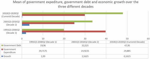
However, the insight gained from (decades 1 and 3). Decade 2 demonstrates that a low level of government expenditure and public the diagram is that the expansionary fiscal policy is failing to meet the objective of the government, since a high level of expenditure and public debt aims to stimulate economic growth, yet it causes the growth to respond negatively debt results in high growth (3,56%). This poses the question whether the Keynesian economic paradigm is valid for South Africa.

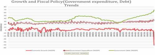
We further analyse the trend of government expenditure, public debt and economic growth covering the period 1972Q1-2021Q2, as is shown in Figure 2. The diagram clearly shows that there is an inverse relationship between government spending, public debt and economic growth, as the graphic analysis demonstrates that, in any instances where the government intervenes through expansionary fiscal policy, it reduces economic growth. Those instances can be observed in; 1973Q2-1979Q4, 1990Q1, 2008Q2- 2010Q4 and 2020Q1- 2020Q2.

Figure 2. Graphic analysis of the trend of economic growth and fiscal variables, 1972Q1-2020Q2.Source: Author’s illustration based on South African Reserve Bank (2020).

When reviewing the literature, we found different views on which variable best captures the fiscal stance between government spending, taxation and deficits. So far no variable among these has been singled out as the most representative of the fiscal policy. Numerous scholars have adopted expenditure as a proxy for fiscal stance. Those scholars include Barro (1990), Zungu et al. (2020), and Zungu and Greyling (2021). Others adopted tax rate (Engen & Skinner, 1996; Rebelo, 1991). Lastly, Easterly and Rebelo (1993) and others used government deficit as a measure of fiscal stance. Moreover, the extant literature on this subject is vast and has capitulated extensive conflicting outcomes, where some authors found a negative relationship between expenditure and growth (Afonso and Sousa, 2011; Karagoz & Keskin, 2015; Makhoba et al., 2019), some found the the relationship to be positive (Babalola, 2015; Bobasu, 2016; Boiciuc, 2014; Masca et al., 2015; Pashourtidou et al., 2014), some found a nonlinearity relationship (Abd-Rahman et al., 2019; Pelin & Taner, 2017; Rana & Hasan, 2016; Zungu & Greyling, 2021; Zungu et al., 2020), and some found the relationship to be inconclusive (Olaoye et al., 2020). The reasons behind these conflicting findings are implausible. Empirically, the feasible explanation for the divergent results in the existing literature lies in the model specifications adopted, and the level of economic development and data sets used in examining the relationship between fiscal policy and economic growth.

This study extends the existing literature on this subject by examining the impact of its fiscal policy on the South African economy. The current study embraces the definition that “fiscal policy refers to the adjustment made by government through government spending, taxation and deficit to achieve certain macroeconomic objectives”, understanding that growth is one of the most important macroeconomic objectives on which the government focuses (Blanchard, 2010). The current study seeks to adopt government spending and public debt to capture fiscal stance, since the government makes use of this component of the fiscal policy to respond to the economic down-turn.

Lin Oo (2019) investigated the impact of fiscal policy on economic growth in Myanmar, using the ordinary least squares (OLS) method with annual data from 1979 to 2016. In their analysis they adopted government expenditure, public deficit and economic growth. Their study reveals a statistically significant relationship between the country’s fiscal deficit and economic growth, which confirms Keynesian assumptions. In their analysis, major macroeconomic variables, such as gross fixed-capital formation, that impact the common-man directly or indirectly, were not captured. In addition, their analysis used annual timeseries data. The current study seeks to contribute to the South African literature by developing a BVAR approach with hierarchical priors using South African quarterly time series data covering the period 1972Q1–2020Q2.

We developed the BVAR with hierarchical priors because of two measured defects, namely when the quality of the data is questionable and when it is typically short. Prior selection in a BVAR is useful in accounting for these weaknesses. Furthermore, the advantage of estimating the current matter with Bayesian techniques is that the impulse response function are more precise. The study by Lin Oo (2019) did not account for these shortfalls. It is on this premise that we seek to fill the gap in the literature by incorporating and examining the effect of these macroeconomic variables on economic growth, which has not been captured in the African studies on the same subject. In addition, the time coverage of our timeseries datasets compares to that in previous studies, making our empirical model robust and useful for policy decision-making. Lastly, the inspiration for this study emanates not only from a lack of studies examining the effects of policy instances on economic growth, but more generally from the fact that this relationship may differ from the one that exists in advanced countries due to the different smoothness in economic development and the macro-economic policies that are being practiced.

2. Review of theoretical and empirical literature

2.1. Theoretical framework

The theoretical model of this study is founded on the analysis carried out by Keynes (1936), which is well-known as the Keynesian theory. The Keynesian theory of development believes that a change by government in the level of government expenditure and taxation positively influences the aggregate demand, which then influences economic activities. The argument made by the Keynesian theory is that fiscal policy through government expenditure (expansionary or contractionary) is the main driver of economic growth through aggregate demand. Expansionary measures occur when the government increases expenditure or reduces taxes to stimulate the aggregate demand. The process behind the expansionary fiscal policy is that its translates into a rise in job creation output, which then stimulates economic growth. However, when the level of the economy is high, the government applies the fiscal policy through contractionary measures by raising tax rates or cutting government expenditure (Blanchard, 2010).

Contrary to Keynes (1936), Wagner (1890) argues that a significant factor that drives fiscal policy is economic growth. This argument was empirically tested by Ismal (2011) in Indonesia, where it was found that both the Keynes and Wagner laws hold. This further intensifies the argument that it is essential to assess both of these theories first, before identifying the main agents of economic development for the purpose of accurate economic policy prescriptions.

The current study adopts the Keynesian theory of economic development as theoretical foundation for the study of variable selection and empirical investigation. Mathematically, the Keynesian function can be expressed as:

(1) $y_t=f\left(X_t\right)+{\epsilon }_t$(1)

The equation above, according to Keynes (1936), is that $y_t=ECON$ (real gross domestic product) and $X_t=GEXPED$ (government expenditure). There are certain aspects of government expenditure that account for a positive impact on economic growth. According to Di-Matteo (2013) an intervention by government to promote economic growth and remedy the market’s failure, is the provision of public goods to stimulate economic growth.

2.2. Empirical literature

After reviewing the literature, we found that the major part of the existing literature dealing with the impact of fiscal policy on economic growth is essentially anchored in two broad strands. However, it is significant to note that there are other variant positions in each broad strand that are fundamentally related, but with some improvements. The Keynesian view posits that consumption is the driver of the economy (Blinder & Solow, 2005), while the classical view posits that “every dollar increase in real government spending is offset by a dollar reduction in private spending”, so crowding out is complete (Dornbusch et al., 1998). The argument of the classical view is that asserts that affect government expenditure are temporary and not effective in the long run when there are adjustments to the prices while employment and output are at their optimum level. Essential to this discussion is the question of the influence of fiscal policy. After scrutinizing the literature, we found that there are three different views onwhich variable best captures the fiscal stance between the three fiscal policy instruments: government spending, taxation and deficits. The literature does not single out which variable among these is most representative of the fiscal policy. Some authors adopted expenditure (Barro, 1990), and others taxation (Stokey & Rebelo, 1995), while still others used deficit (Stokey & Rebelo, 1995) to capture the fiscal stance.

Barro (1990) studied the impact of fiscal policy on economic growth in a panel of 47 countries in the post World War II period, finding fiscal policy to have a positive effect on economic growth. The inconsistency emerged when Engen and Skinner (1992) documented that fiscal policy decreased economic growth in a panel of 107 countries. The findings reported by Barro (1990) and Engen and Skinner (1992) further contradicted the results documented by Ali (2005) in a panel data of 90 countries covering the period 1975–1998, as this author found that the effect of fiscal policy on economic growth is inconclusive.

Afonso and Sousa (2011) studied the impact of fiscal policy on macroeconomic structure in Portugal, using a BSVAR approach over the period 2003Q1-2015Q2. Their findings supported the argument by Engen and Skinner (1992). In the South African context, the study by Charl et al. (2013) used South African data covering the period 1970Q1-2009Q4, employing the calibrated DSGE, SVECM and TVP-VAR models. Their study documented that fiscal policy is positively related to economic growth, supporting the results documented by Barro (1990). A further contradiction emerged in the South African literature when the study carried out by Makhoba et al. (2019) found that there is a negative relationship between fiscal policy and economic growth in the long run, using the VECM approach in examining the short-long run effect of the fiscal policy on economic variables covering the period 1960–2017. The findings documented by Makhoba et al. (2019) supported the findings reported by Boiciuc (2014) in a case study of the Romanian economy, using the SVAR technique and covering the period 2000Q1-2012Q4.

Masca et al. (2015) studied the impact of fiscal policy as a growth engine in the European Union (EU) economies using the GLS and the FGLS, covering the period 1995–2011. Their findings pointed out that the dimension of the public sector improves economic growth by improving investment and government revenue. These findings were further supported by the findings reported by Babalola (2015) in the case of Nigeria, covering the period 1981–2013, and Bobasu (2016) using a BVAR in the Romanian economy, covering the period 2000Q1 to 2014Q2.

Looking at the most recent literature, the study conducted by Olaoye et al. (2020), used the GMM techniques to account for simultaneity and endogeneity problems inherent in the dynamic model, covering the period 1980–2017 in Nigeria. Their findings revealed that there is evidence of asymmetry in the government spending and economic growth relationship in Nigeria over the period of study. Rohimah et al. (2020) studied the impact of fiscal policy on economic growth at a regional level in North Sumateran provinces, covering the period 2011Q1-2017Q4. Their study adopted two components of fiscal policy: government expenditure and tax revenue, to measure the fiscal policy. In their study they documented that the fiscal policy has a negative impact on income inequality in North Sumatera, which then contradicts the arguments made by Barro (1990) and Masca et al. (2015).

3. Methodological framework

3.1. Justification of variables

This study employed quarterly time series covering the period 1972Q1-2020Q2 to estimate a BVAR model. The current study used variables suggested in the literature and also included gross fixed capital formation, which impacted growth in various countries directly or indirectly but was not captured in the Lin Oo (2019) model.Our variables include GDP at a factor cost of the non-agricultural sector (ECON), national government expenditure as % GDP (EXPEN), total debt of government as % of GDP (PDEBT), and gross fixed-capital formation (INVEST), obtained from the South African Reserve Bank. According to the Keynesian theory of public debt, an increase in government expenditure fuels domestic activity and crowds in private invensmest. Therefore, increasing government spending is positively related to national output, which then leads to employment (Makin, 2015). While public debt is thought to be negatively related to economic growth, as the public debt overhang suggests, unsustainable public debt undermines the credibility of state policy, obstructing government commitment to policy actions.Again, the use of public debt to finance public investment will drain the liquidity from the market.

All our variables were selected in line with the theoretical foundations and empirical literature underpinning the relationship under investigation. We adopted the unit root test within the bvar () function.

3.2. Bayesian VAR model: Model specifications

To achieve the objective of the study, we adopted a Bayesian VAR (BVAR) approach, following the example of Bańbura et al. (2010), with all the mathematically detailed technical Bayesian VAR. However, our BVAR model accommodated hierarchical priors for various reasons. Reflect on the following VAR(p) model:

(2) $y_t={\alpha }_0+{\mathrm{A}}_1{y}_{\mathrm{t}-1}+\dots +{\mathrm{A}}_{\mathrm{p}}{\mathrm{y}}_{t-p}+{\in }_{t}with{\in }_t\tilde{N}\left(0,\mathrm{\Sigma }\right)$(2)

where $y_t=ECO{N}_t,EXPE{N}_t,PDEB{T}_t,INVES{T}_t$ is a $4\times 1$ column vector of 4 endogenous variables in the BVAR system, while ${\alpha }_0$ denotes a $4\times 1$ vector of the intercept. ${\mathrm{A}}_{\mathrm{j}}\left(J=1,\dots ,p\right),$ denoting a $4\times 4$ matrix of autoregressive coefficients of regressors, $p$ is the order of the BVAR and, finally, ${\in }_t$ is a $4\times 1$ vector of Gaussian exogenous shocks with a zero mean and variance covariance (VCOV) matrix Σ. The $4+{4^2}_p$ are the number of coefficients to be estimated, rising quadratically with the number of included variables and linearly in the lags order. Such parameterization leads to inaccuracies with regard to structural inference and out-of-sample prediction, especially for higher-dimensional models. This phenomenon is normally referred to as the curse of dimensionality.

The good fit of the VAR estimated through the Bayesian approach, is that it tackles this limitation by means of an impressive extra structure in the model, which includes the priors which have been shown to be effective in militating the curse of dimensionality, and allows for a large model to be estimated (Bańbura et al., 2010; Doan et al., 1984). They push the model parameters towards a parsimonious benchmark, reducing estimation errors and improving out-of-sample projection accuracy (Koop, 2013). This shrinkage is associated with the frequentist regularization approaches (De-Mol et al., 2008; Hoerl & Kennard, 1970). Our approach is flexible and significant in accommodating a varied range of naturally involved prior information, economic issues, and the issuing of data, and it is also powerful in mitigating uncertainty through hierarchical modelling (Gelman et al., 2013).

3.3. Selection of hierarchical priors and specification

Properly informing prior beliefs is critical, and thus the subject of much research. The flat priors come from the multivariate context, which posits that the priors impose a certain belief that aims to yield poor inference (Bańbura et al., 2010; Sims, 1980) and inadmissible estimators. Going as far back as the study by Litterman (1980), he contributed to the argument of the priors set-up by setting their hyperparameters in a way that maximizes the out-of-sample prediction of performance over a pre-sample. While the study by Del-Negro and Schorfheide (2004) chose values that maximize the marginal data density, the study by Bańbura et al. (2010) adopted a slightly different approach, following Litterman (1980) by controlling for overfitting and using in-sample fitting as their choice. Economic theory is an ideal foundation for priors information, but it is lacking in many settings, in particular in high-dimensional models. Villani (2009) rebuilt the model further by placing the priors in the steady state, which was then better understood theoretically by economists. The study by Giannone et al. (2015) suggested the setting of hyperparameters in a data-based fashion by treating them as additional parameters. In their approach, uncertainty surrounding their choice of prior hyperparameters is acknowledged explicitly, which then ─ invoking Bayes’ Law ─ can be expressed as:

(3) $p\left(\gamma |y\right)\propto p\left(y|\theta ,\gamma \right)p\left(\theta |\gamma \right)\mathrm{p}\left(\gamma \right)$(3)

(4) $p\left(Y|\gamma \right)={\int }^p\left(y|\theta ,\gamma \right)p\left(\theta |\gamma \right)\mathrm{d}\theta$(4)

where $y=\left(y_p+1,\dots ,y_T\right)\mathrm{\top },$ the variance and autoregressive parameters of the VAR are indicated by $\theta$, and the set of hyperparameters by $\gamma$. The first part of Equation 2(2) $y_t={\alpha }_0+{\mathrm{A}}_1{y}_{\mathrm{t}-1}+\dots +{\mathrm{A}}_{\mathrm{p}}{\mathrm{y}}_{t-p}+{\in }_{t}with{\in }_t\tilde{N}\left(0,\mathrm{\Sigma }\right)$(2) is marginalized with respect to the parameters $\theta$ in Equation 3(3) $p\left(\gamma |y\right)\propto p\left(y|\theta ,\gamma \right)p\left(\theta |\gamma \right)\mathrm{p}\left(\gamma \right)$(3) . This produces a density of the data as a function of the hyperparameters $p\left(y|\gamma \right),\mathrm{a}\mathrm{n}\mathrm{d}$ also the marginal likelihood (ML). The quantity is conditional to the hyperparameters $\gamma ,$ but marginal with respect to parameters $\theta$. A decision criterion for maximization and hyperparameter choice is derived from the results of the ML test, which constitutes an empirical Bayes method, with clear frequentist interpretation (Giannone et al., 2015). In our approach, the ML is adopted to explore the full posterior hyperparameter space, to acknowledge the uncertainty that surrounds it. Giannone et al. (2015) claim that this produces results that are robust and theoretically grounded, if implemented in an efficient manner. The authors established high accuracy of forecasts and impulse response functions, with the model performing competitively compared to factor models. Since then their approach has been used widely in applied research (Altavilla et al., 2018; Miranda-Agrippino & Rey, 2015). The contribution made by Giannone et al. (2015) emphasizes conjugate prior distributions of the Normal-inverse-Wishart (NIW) family, to be precise. Conjugacy involves that the ML is available in closed form, allowing competent computation, where the NIW family embraces numerous of the most frequently used priors (Koop & Korobilis, 2010), with some notable exceptions. These include the Dirichlet-Laplace prior (Bhattacharya et al., 2015), the steady-state prior (Villani, 2009) and the Normal-Gamma prior (Huber & Feldkircher, 2019). The recent contributors to this argument focus on accounting for heteroskedastic error structures (Clark, 2011; Kastner & Fruhwirth-Schnatter, 2014). This may improve model performance, but is not possible within the conjugate setup and, moreover, would confuse inference. In the selected NIW framework we approach the model in Equation 1(1) $y_t=f\left(X_t\right)+{\epsilon }_t$(1) by letting $A={\left[a0,A1,\dots ,Ap\right]}^{\prime }$ and $\beta =vec\left(A\right).$ Then the conjugate prior setup reads as follows:

(5) $\beta |\mathrm{\Sigma }\sim \hspace{0.17em}\left(b,\mathrm{\Sigma }\otimes \mathrm{\Omega }\right)$(5)

(6) $\mathrm{\Sigma }\sim I\mathcal{W}\left(\mathrm{\Psi },d\right)$(6)

where $b,\mathrm{\Omega },\mathrm{\Psi }$ and $d$ are functions of a lower dimensional vector of hyperparameters $\gamma$. Giannone et al. (2015) considered three priors in their study, which were called the sum-of-coefficients prior, the single unit-root prior, and the Minnesota (Litterman) prior that is used as a baseline. In his study, Litterman (1980) adopted the Minnesota prior and imposed the hypothesis that individual variables all follow random-walk processes. This parsimonious specification typically performs well in forecasts of macroeconomic time series (Kilian & Lütkepohl, 2017) and is often used as a benchmark to evaluate accuracy. The prior is characterized by the following moments:

(7) $\begin{array}{rl}& \mathrm{E}(A_s{)}_{ij}|\mathrm{\Sigma }=\left\{\begin{array}{c}1,andifi=j,s=1\\ 0,andotherwise\end{array}\right.\\ & \end{array}$(7)

(8) $\mathrm{c}\mathrm{o}\mathrm{v}(A_s{)}_{ij}(A_r{)}_{kl}|\mathrm{\Sigma }=\left\{\begin{array}{c}{\lambda }^2\frac{1}{s^{\sigma }}\frac{{\mathrm{\Sigma }}_{jk}}{{\mathrm{\Psi }}_j/\left(d-m-1\right)},andifl=jandr=s\\ 0,andotherwise\end{array}\right.$(8)

where $\lambda$ is the key parameter which controls the tightness of the prior and, therefore, weighs the relative significance of data and prior. When the priors are imposed precisely, that will follow $\lambda \to 0$, while when $\lambda \to \mathrm{\infty },$ the posterior estimates will approach the ordinary least squares (OLS) estimates. Finally,$\psi$ controls the prior’s standard deviation on lags of variables other than the dependent variable. The Minnesota prior is normally applied as an additional prior in the model, trying to “reduce the significance of the deterministic component implied by VAR models’ estimated conditioning on the initial observations” (Giannone et al., 2015). The study by Doan et al. (1984) included the sum-of-coefficients (SOC) prior by imposing the notion that a no-change projection is optimal at the beginning of a time series. It is implemented via the Theil mixed estimation by adding artificial dummy observations to the data matrix, which are constructed as follows:

(9) $\underset{M\times M}{y{ }^{+}}=\mathrm{d}\mathrm{i}\mathrm{a}\mathrm{g}\left(\frac{\bar{y}}{\mu }\right)+\underset{M\times \left(1+MP\right)}{x^{+}}=\left[0,y^{+},\dots ,y^{+}\right]$(9)

in Equ. 9(9) $\underset{M\times M}{y{ }^{+}}=\mathrm{d}\mathrm{i}\mathrm{a}\mathrm{g}\left(\frac{\bar{y}}{\mu }\right)+\underset{M\times \left(1+MP\right)}{x^{+}}=\left[0,y^{+},\dots ,y^{+}\right]$(9) , where $\bar{y}$ is a $4\times 1$ vector of the averages over the first p observations of each variable. The variance is controlled by the key parameter μ and, therefore, due to the tightness of the prior for $\mu \to \mathrm{\infty },$ the prior becomes uninformative. For $\mu \to 0$ the model is pulled towards a form with as many unit-roots as variables and no co-integration. This inspires the single unit-root (SUR) prior (Sims & Zha, 1998), which allows for co-integration relations in the data. The prior pushes the variables either towards them, or towards the presence of at least a one-unit root or unconditional mean. These kinds of priors, associated with dummy observations are:

(10) $\underset{1\times M}{\overset{++}{Y}}=\frac{\bar{y}}{\delta }+\underset{1\times \left(1+MP\right)}{x^{++}}=\left[\frac{\bar{y}}{\delta },y^{++},\dots ,y^{++}\right]$(10)

where $\bar{y}$ is again distinct, as above. Likewise, $\delta$ is the key parameter, governing the tightness of the SUR prior. A number of heuristics, proposed as setting this parameter for these priors, have been discussed in various studies, including Doan et al. (1984) and Bańbura et al. (2010). The study by Giannone et al. (2015) noted that, from a Bayesian standpoint, this choice of parameters is theoretically identical to the implication for any other parameter of the model. “They show that it is possible to treat the model as a hierarchical one, with the marginal likelihood of the data, given the prior parameters, available in closed form for VAR models with conjugate priors” (Giannone et al., 2015). Estimating these hyperparameters via maximization of the ML, is an empirical Bayes method with a clear frequentist interpretation (Giannone et al., 2015).

4. Empirical analysis and interpretation results

This section discusses the empirical results of the entire study with regard to the impact shock of fiscal-policy variables on economic growth in South Africa. The findings of the study will be robust to policy-makers in understanding the impact shock of either the contractual or expansionary fiscal policy on the South African economy. This will also be useful in understanding the sustainability of unexpected shocks in South Africa’s economy. As part of the preliminary analysis we used the fred-transform () function for data transformation and the stationarity test, as it is one of the most important tasks to be performed before estimating the BVAR model.

4.1. Data transformation and stationarity

Developing a BVAR model, using the function bvar (), requires the data to be coercible to a rectangular numeric matrix with no missing data points. We used 4 variables in our BVAR model, these variables being: ECON, EXPEN, PDEBT and INVEST. GDPp is given in billions of 2010 dollars, while other variables are in rates, except for Gini which is an index. We followed the transformation adopted by Kuschnig and Vashold (2019) to transform all the variables to log levels, in order to demonstrate dummy priors. Our transformation was performed through the function fred-transform (). This function supports the transformation that appeared in McCracken and Ng (2016), which can be accessed via their transformation codes, and automatic transformation. We then used the codes argument derived from the direct-transformation codes. Doing this helped us to choose 5 log-differences for investment and 2 for 1^st differences. We then set the number of lags to 4 for yearly differences of our quarterly data.

4.1.1. The prior setup and configuration

The traditional maximum likelihood VARs (TML-VAR) suffer two major defects, using data from middle and low-income countries where the quality of the data is questionable and typically short. The TML-VAR are over-pameterised where too many lags are included in the model, leading to a significant loss in the degree of freedom. Therefore, priors selection in a BVAR is useful in accounting for this weakness of the TML-VAR. After having prepared the data, we then specified priors and configured our model by using the bv_priors () function, which holds arguments for the Minnesota and dummy-observation priors, as well as the hierarchical treatment of their hyperparameters. We began by adjusting the Minnesota prior. The prior hyperparameter $\lambda$ has a Gamma-hyperprior and is handed upper and lower bounds for its Gaussian proposal distribution in the MH step. As a result, we started by not treating $\alpha$ hierarchically. Following Kuschnig and Vashold (2019), we let $\mathrm{\Psi }$ be set automatically to the square root of the innovation variance, after fitting $AR\left(p\right)$ models to each of the variables. We then included a sum-of-coefficients in a single unit-root prior, where we had pre-constructed three dummy observation priors. The hyperpriors of their key parameters are assigned Gamma-distributions, with specifications working similar to those for $\lambda$. In this version of the BVAR, this will be equivalent to providing the character vector $c\left(Lambda,Soc,Sur\right)$, after setting the configuration of the model’s priors and Metropolis-Hastings.

4.2. Estimation of the model

We estimated our model using the function bvar (),also noting that this function needed us to prepare the data and provide the lag order of p as arguments. The study also passed the customization setup with respect to the argument, and we defined the total number of initial iterations to be discarded with n_burn and those with n_draws. The number of burn and draws were set to 15,000 and 5000, respectively. When our model was estimated, where we set the verbose = TREUE in the bvar() function, it enabled a progress bar during the MCMC step. Table 1 sums up the results of the posterior marginal likelihood.

Table 1. Posterior marginal likelihood

Optimisation concluded. Posterior marginal likelihood: −1716.465. Hyperparameters: lambda = 1.49452; soc = 0.246702; sur = 0.35986. ||==================================================| 100%. Finished MCMC after 20.3 secs.

Source: Author’s calculation based on South African Reserve Bank (2020).

The return value of the BVAR function is an object of a class that produces several outputs, including the parameters of interest, which are hierarchically treated hyperparameters, the VCOV matrix and the posterior draws of the VAR coefficients. The object of the BVAR also contains the values of the ML¹ for each draw, the prior settings provided, the starting values of the prior hyperparameters obtained from optima as well as the ones set automatically, and the original call to the bvar() function.

4.2.1. Analysing outputs

The BVAR model contains a range of standard methods for the model. We assessed the overview and convergence of the MCMC algorithm of our estimation, which is significant for its stability. Table 2 provides a summary of the BVAR model, where the coefficients of lambda, soc and sur are 1.513, 0.126, and 0.476, respectively, while the iterations (burnt/thinning): 15,000 (5000/1) and the accepted draws (rate) are found to be 39%. The arguments var_response and var_impulse provide a concise alternative way of retrieving autoregressive coefficients.

Table 2. Summary of the BVAR model

Bayesian VAR consisting of 238 observations, 4 variables and 4 lags. Time spent calculating: 16.89 secs. Hyperparameters: lambda, soc, sur. Hyperparameter values after optimisation: 1.513, 0.126, 0.476. Iterations (burnt/thinning): 25,000 (8000/1). Accepted draws (rate): 3933 (0.393).

Source: Author’s calculation based on South African Reserve Bank (2020).

We then used the type of argument to choose a specific type of plot, as it shown in Figure 3, which provides plots of the density, trace of the ML and hierarchically treated hyperparameters.

Figure 3. Trace and density plots of all hierarchically treated hyperparameters and the ML.Source: Author’s calculation based on South African Reserve Bank (2020).

The graphical inspection of density and trace plots signifies convergence of the key hyperparameters in the estimated BVAR model. The chain appears to be exploring the posterior rather well; no glaring outliers are recognizable.

4.2.2. Impulse responses of the Bayesian VAR

This study aims to identify the impact of government expenditure and public debts shocks on economic growth, and to examine whether the shocks are persistent covering the period 1972Q1-2020Q2, using a BVAR with hierarchical priors selection. Figure 4 reports the impulse responses of economic growth (ECON), government expenditure (% GDP) (DGEXPED), government debt (% GDP) (DPDEBT) and investment (DLGFCF). The shaded areas refer to the 90% and the 68% credible sets. The responses in Figure 4 reflect on the basis of the model with hierarchical priors selection, where the coefficients for the dynamic impact of DGEXPED, DPDEBT, DLGFCF on economic growth have been given a tighter hierarchical priors distribution.

Figure 4. Generated impulse responses of the Bayesian VAR.Source: Author’s calculation based on South African Reserve Bank (2020).

The second graph of the IRF’s plots in the first row shows that economic growth (ECON) responds negatively to an unexpected 1% shock on government spending, and the response is significant and persistent. Government expenditure (DGEXPED) initially has a gradually declining impact on economic growth (ECON) of about 0.25% from period zero to period two. This then converges to positive, but below the steady-state region, after which it reverses back to a steady-state region. The impulse response signifies that the impact of an unexpected shock on government expenditure lasts for a longer period of time, which is estimated to be 10 lags. This further supports what has been observed in Figures 1 and 2 in the first section.

The results are plausible and consistent with the existing literature such as that of Karagoz and Keskin (2015) for Turkey; Babalola (2015) for Nigeria, and Makhoba et al. (2019) for South Africa.

The argument behind the negative impact of government expenditure on the South African economy is twofold: 1) It is due when there is an injection of government spending, which contributes towards an increase in interest rates. These high interest rates lead to a crowding-out effect on private investment. Thus, government expenditure is subject to the law of diminishing returns, which means additional expenditure will result in a decline in the economic growth rate. Consequently, economic fragility would be expected if the country is facing such a process, which will automatically lower investment and then disturb the competent distribution of resources. 2) It could be that a large portion of government expenditure is directed towards social consumption (healthcare systems, public education, and social security) in South Africa rather than productive economic institutions like investing in technological advancement and innovation and infrastructure development, which are more crucial to promoting long-term economic growth in developing countries.

A further decline was reported in economic growth as the result of an unexpected shock to public debt. Following a one percent standard deviation shock to public debt (DPDEBT), has a gradually declining impact on economic growth (ECON) of about 0.6% from period zero to period two, then converges to a positive but below the steady-state region, then reverses back to the steady-state region.The impulse response signifies that the negative impact of an unexpected shock on public debt lasts for a longer period of time but dies after 10 lags, and the shock is significant and persistent. The results further support what had been observed in Figures 1 and 2 in the first section. The results are plausible and consistent with several economic literatures (Sokbae et al., 2017 for advanced countries; Ndoricimpa, 2020 for African economies). The logic behind the negative impact of public debt on the South African economy could be that the accumulation of public debt as a result of fiscal measures taken to stimulate economic activity during the global financial and economic crises of 2008 can be associated with a potential negative effect on future economic growth and stability (Mencinger et al., 2015).

Lastly, a positive response in economic growth was reported as a result of an unexpected shock on investment (DLGFCF). Following a 1% standard deviation shock on DLGFCF initially had a positive impact on economic growth (ECON) of about 0.25% from period zero to period two. This then converged to a negative, but above the steady-state region, after which it reversed back to a steady-state region. This impulse response signifies that a positive impact of an unexpected shock on investment lasts for a longer period, but dies after 8 lags and the shock is significant. The results are plausible and consistent over several studies such as Pelin and Taner (2017) and Zungu et al. (2020). The argument is that the neoclassical theory assumes that the economy grows at a constant rate, implying that more investment is required for labour productivity. This implies that the growth rate of output in the steady state is exogenous and independent of the saving rate (Dornbusch et al., 2014). In addition, the neoclassical theory asserts that technological progress enhances the productivity of labour. Finally, the neoclassical theory believes in convergence, which means that if countries have the same population growth, saving rate and production function, they will attain the same level of output. This means that countries are poor due to lack of capital; however, should they save like richer countries and have technological access they would be on par (Domar, 1946).

4.2.3. Unconditional forecasts of the Bayesian VAR for 2.5 years prior

We further generate unconditional forecasts of the endogenous variables for a 2 years and 6 months period prior to the mean adjusted BVAR, following Kuschnig and Vashold (2019), as demonstrated in Figure 5. The unconditional forecasts are for economic growth, government spending, government debt and investment. The shaded areas refer to the 90% and the 68% credible sets. According to our model, economic growth (ECON) is expected to continuously decrease to about 40% in the next 10 quarters (2 years and 6 months).

Figure 5. Unconditional forecasts for all variables employed in this study.Source: Author’s calculation based on South African Reserve Bank (2020).

This finding signifies the disaster incurred in our economy as a result of the current health crisis (COVID 19). Government expenditure seems to be not clear on how it is going to behave in the next 10 quarters (2 years and 6 months), as its impact is not significant. Over the same period the unconditional forecasts show that government debt is expected to continuously rise to above 15% of GDP for the next 10 quarters (2 years and 6 months). It is not surprising to see that the unconditional forecasts of the investment show that the investment is expected to decrease to approximately 55% in the next 10 quarters (2 years and 6 months). The results illustrate that the South African economy seems to be more exposed to shocks in fiscal policy, affecting both economic growth and investment.

4.3. Conclusion and policy recommendation

The current study provides sufficient evidence of a significant negative relationship between government expenditure and government debt and economic growth in South Africa. The findings of the study yield that economic growth responds negatively to an unexpected shock on fiscal policy (through government expenditure and public debt) and its impact is significant and persistent. The results are plausible and consistent with the existing literature such as Masca et al. (2015) for EU economies, Babalola (2015) for Nigeria, Bobasu (2016) for Romania and Olaoye et al. (2020) for Nigeria. However, the response was felt after 4 period lags and further sustained for a long-term period. The results further validate the importance of investment in uplifting the South African economy, as it shows that investment is an important driver of growth in South Africa, since there is a positive response in economic growth as a result of an unexpected shock on investment.

We also take the BVAR analysis forward by generating a 10 quarters (2 years and 6 months) period of unconditional forecasts for the endogenous variables, using the mean adjusted BVAR, following Kuschnig and Vashold (2019). The unconditional forecasts for the mean adjusted BVAR demonstrate that both economic growth and investment are expected to experience a severe decline in the near future, over a 10 quarters (2 years and 6 months) period, while public debt is expected to experience a sharp increase. The forecast for government expenditure is ambiguous.

The study proposes that policy-makers should focus on promulgating macroeconomic policies that will attract investment consistent with job creation and economic expansion in South Africa’s economy. This further supports the fact that the South African economy does not need more government intervention through expansionary fiscal policy in the form of excessive government expenditure, as that tends to cause economic contraction. Furthermore, a conducive and investment-friendly environment is paramount, which would then be expected to create more jobs, and ultimately promote long-term sustainable economic growth in the South African economy. The current study was limited in its ability to identify the impact shock of fiscal policy variables on economic growth in South Africa. However, there is a growing body of literature that believes that there is nonlinearity between fiscal policy variables and economic growth. Therefore, we suggest that future research should focus on a comparative study where South Africa is compared to emerging economies. The STA model will be appropriate in finding the threshold effect in a time series context.

Disclosure statement

No potential conflict of interest was reported by the author(s).

Additional information

Funding

The authors received no direct funding for this research

Notes on contributors

Lindokuhle T Zungu

Lindokuhle Talent Zungu is a junior lecturer in the Department of Economics at the University of Zululand. In 2021, he was selected as an Associate Member of the Pan-African Scientific Research Council. In the same year, he received an award for being the best master’s candidate in the Economics department (University of Zululand) by Economic Research Southern Africa (ERSA).

In 2019, because of his being an avid researcher, he was elected to participate in the SA-TIED young scholar programme (South Africa) under the United Nations University-World Institute for Development Economics Research (UNU-WIDER). In 2017, he was appointed as a researcher for Professor Greyling. He is an avid researcher, and his work has been published in accredited journals of economics and also as working papers under the ERSA working paper series. He received his education at the University of Zululand (UNIZULU) with a Master’s in commerce (Economics) and is currently registered for a Doctorate Degree in Economics at UNIZULU. His research interest is in macroeconomics.

References

- Abd-Rahman, N. H., Shafinar-Ismail, S., & Ridzuan, A. R. (2019). How does public debt affect economic growth? A systematic review. Cogent Business and Management, 6(1), 1701339. https://doi.org/10.1080/23311975.2019.1701339
- Afonso, A., & Sousa, R. M. (2011). The macroeconomic effects of fiscal Iolicy In Portugal: A BAyesian SVAR analysis. Portuguese Economic Journal, 10(1), 61–16. https://doi.org/10.1007/s10258-011-0071-2
- Ali, A. M. (2005). Fiscal policy and economic growth: The effect of fiscal volatility. Journal of Business & Economics Research, 3(5), 18–25. http://dx.doi.org/10.1108/01443581111161841
- Altavilla, C., Boucinha, M., & Peydro, J. L. (2018). Monetary policy and bank profitability in a low interest rate environment. Economic Policy, 33(96), 531–586. http://dx.doi.org/10.1093/epolic/eiy013
- Babalola, A. (2015). Fiscal policy and economic development in Nigeria. Journal of Economics and Sustainable Development, 6(7), 2015. https://doi.org/10.2307/19-5364
- Bańbura, M., Giannone, D., & Reichlin, L. (2010). Large Bayesian vector auto regressions. Journal of Applied Econometrics, 25(1), 71–92. https://doi.org/10.1002/jae.1137
- Barro, R. J. (1990). Government spending in a simple model of endogenous growth. Journal of Political Economy, 98(1), 103–125. https://doi.org/10.1086/261726
- Begg, D., Vernasca, G., Fischer, S., & Dornbusch, R . (2014). Economics, ondon [etc.]: McGraw-Hill education, cop. 11th edition, 1 (XXII), 708.
- Bhattacharya, A., Pati, D., Pillai, N. S., & Dunson, D. B. (2015). Dirichlet–laplace priors for optimal shrinkage. Journal of the American Statistical Association, 110(512), 1479–1490. https://doi.org/10.1080/01621459.2014.960967
- Blanchard, O . (2010). Macroeconomics. Prentice Hall.
- Blinder, A. S., & Solow, R. M. (2005). Do fiscal policies matter? In A. Bagchi (Ed.), Readings in public finance. Oxford University Press. pp. 283–300.
- Bobasu, A. (2016). Quantifying the impact of fiscal policy on economic growth in the Romanian economy: A Bayesian approach. Journal of Economics, Business and Management, 4(1), 72–75. https://doi.org/10.7763/JOEBM.2016.V4.369
- Boiciuc, I. (2014). The macroeconomic effects of fiscal policy: A BVAR approach, Review of Economic & Business Studies, 7(2), 163–169. http://rebs.feaa.uaic.ro/articles/pdfs/214.pdf
- Charl, J., Liu-Guangling, L., & Ruthira, N. (2013). Analysing the effects of fiscal policy shocks in the South African economy. Economic Modelling, 32(C), 215–224. https://doi.org/10.1016/j.econmod.2013.02.011
- Clark, T. E. (2011). Real-time density forecasts from Bayesian vector autoregressions with stochastic volatility. Journal of Business & Economic Statistics, 29(3), 327–341. https://doi.org/10.1198/jbes.2010.09248
- Del-Negro, M., & Schorfheide, F. (2004). Priors from general equilibrium models for VARs. International Economic Review, 45(2), 643–673. https://doi.org/10.1111/j.1468-2354.2004.00139.x
- De-Mol, C., Giannone, D., & Reichlin, L. (2008). Forecasting using a large number of predictors: Is Bayesian shrinkage a valid alternative to principal components? Journal of Econometrics, 146(2), 318–328. https://doi.org/10.1016/j.jeconom.2008.08.011
- Di-Matteo, L. (2013). Measuring government in the twenty-first century: An international overview of the size and efficiency of public spending. Fraser Institute Retrieved October 3, 2020, from www.fraserinstitute.org
- Doan, T., Litterman, R., & Sims, C. (1984). Forecasting and conditional projection using realistic prior distributions. Econometric Reviews, 3(1), 1–100. https://doi.org/10.1080/07474938408800053
- Domar, E. D. (1946). Capital expansion, rate of growth, and employment. In Econometrica (Vol. 14, pp. 137–147), The Econometric Society. https://doi.org/10.2307/19-5364.
- Dornbusch, R. S., Fischer, R., & Starz, R. (1998). Macroeconomic. USA, McGraw-Hill Companies.
- Easterly, W., & Rebelo, S. (1993). Fiscal policy and economic growth an empirical investigation. Journal of Monetary Economics, 32(3), 417–458. https://doi.org/10.1016/0304-3932(93)90025-B
- Engen, E. M., & Skinner, J. (1996). Taxation and economic growth. National Bureau of economic research working paper, Massachusetts Avenue Cambridge, MA. https://www.nber.org/system/files/working_papers/w4223/w4223.pdf
- Engen, E. M., & Skinner, J. (1996). Taxation and economic growth. National Tax Journal, 49(4), 617-–42. https://doi.org/10.1086/NTJ41789231.
- Gelman, A., Carlin, J. B., Stern, H. S., Dunson, D. B., Vehtari, A., & Rubin, D. B. (2013). Bayesian data analysis. CRC Press. https://doi.org/10.1201/b16018
- Giannone, D., Lenza, M., & Premiere, G. E. (2015). Prior selection for vector autoregressions. Review of Economics and Statistics, 97(2), 436–451. https://doi.org/10.1162/REST_a_00483
- Hoerl, A. E., & Kennard, R. W. (1970). Ridge regression: Biased estimation for nonorthogonal problems. Technometrics, 12(1), 55–67. https://doi.org/10.1080/00401706.1970.10488634
- Huber, F., & Feldkircher, M. (2019). Adaptive Shrinkage in Bayesian vector autoregressive models. Journal of Business & Economic Statistics, 37(1), 27–39. https://doi.org/10.1080/07350015.2016.1256217
- Ismal, R. (2011). Assessing economic growth and fiscal policy in Indonesia. East-West Journal of Economics and Business, 14(1), 53–71. https://www.u-picardie.fr/eastwest/fichiers/art94.pdf
- Karagoz, K., & Keskin, R. (2015). Impact of fiscal policy on the macroeconomic aggregates in Turkey: Evidence from BVAR model. Procedia Economics and Finance, 38(2016), 408–420. https://doi.org/10.1016/S2212-5671(16)30212-X
- Kastner, G., & Fruhwirth-Schnatter, S. (2014). Ancillarity-sufficiency interweaving strategy (ASIS) for boosting MCMC estimation of stochastic volatility models. Computational Statistics & Data Analysis, 76(4), 408–423. https://doi.org/10.1016/j.csda.2013.01.002
- Keynes, J.M. (1936). The General Theory of Employment, Interest, and Money. International Relation and Security Network New York:Harcourt, Brace and Co. https://www.files.ethz.ch/isn/125515/1366_KeynesTheoryofEmployment.pdf
- Kilian, L., & Lütkepohl, H. (2017). Structural vector autoregressive analysis. Cambridge University Press.
- Koop, G. M. (2013). Forecasting with medium and large Bayesian VARS. Journal of Applied Econometrics, 28(2), 177–203. https://doi.org/10.1002/jae.1270
- Koop, G. M., & Korobilis, D. (2010). Bayesian multivariate time series methods for empirical macroeconomics. Foundations and Trends in Econometrics, 3(4), 267–358. https://doi.org/10.1561/0800000013
- Kuschnig, N., & Vashold, L. (2019), Bayesian vector autoregressions with hierarchical prior selection in Rstudio. Department of Economics Working Paper, wirtschafts univesirty, Austria.
- Lin Oo, T. (2019). The effect of fiscal policy on economic growth in Myanmar. East Asian Community Review, 2(1), 101–124. https://doi.org/10.1057/s42215-019-00020-6
- Litterman, R. B. (1980). A Bayesian procedure for forecasting with vector autoregressions. Working Paper, Massachusetts Institute of Technology, Cambridge, USA.
- Makhoba, B. P., Kaseeram, I., & Greyling, L. (2019). Assessing the impact of fiscal policy on economic growth in South Africa. African Journal of Business and Economic Research, 14(1), 7–29. https://doi.org/10.31920/1750-4562/2019/V14n1a1
- Makin, A. J. (2015). Has excessive public debt slowed world growth? World Economics, 16(1), 1–17. https://ideas.repec.org/a/wej/wldecn/629.html
- Masca, S. G., Cuceu, I. C., & Vaidean, V. L. (2015). The fiscal policy as growth engine in EU countries. Procedia Economics and Finance, 32(2015), 1628–1637. https://doi.org/10.1016/S2212-5671(15)01489-6
- McCracken, M. W., & Ng, S. (2016). FRED-MD: A monthly database for macroeconomic research. Journal of Business & Economic Statistics, 34(4), 574–589. https://doi.org/10.1080/07350015.2015.1086655
- Mencinger, J., Aristovnik, A., & Verbic, M. (2015). Revisiting the role of public debt in economic growth: The case of OECD countries. Inzinerine Ekonomika-Engineering Economics, 26(1), 61–66. http://dx.doi.org/10.5755/j01.ee.26.1.4551
- Miranda-Agrippino, S., & Rey, H. (2015). World asset markets and the global financial cycle”, National Bureau of economic research working paper, Centre for economic policy Research. Retrieved February 10, 2020, from cepr.org/active/publications/discussion_papers/dp.php?dpno=10936
- Ndoricimpa, A. (2020). Threshold effects of public debt on economic growth in Africa: A new evidence. Journal of Economics and Development, 22(2), 187–207. https://doi.org/10.1108/JED-01-2020-0001
- Olaoye, O. O., Okorie, U. U., Eluwole, O. O & Fawwad, M.B. (2020). Government spending shocks and economic growth: Additional evidence from cyclical behaviour of fiscal policy. Journal of Economic and Administrative Sciences, 37(4), 419–437. https://doi.org/1026-4116.10.1108/jeas-01-2020-0003.
- Pashourtidou, N., Savva, C. S., & Syrichas, N. (2014). The effects of fiscal consolidation on macroeconomic indicators in Cyprus. Cyprus Economic Policy Review, 8(1), 93–119. https://www.ucy.ac.cy/erc/documents/Pashourtidou_Savva_Syrichas_93-119.pdf
- Pelin, V. I., & Taner, T. (2017). Government size and economic growth in Turkey: A threshold regression analysis. Prague Economic Papers, 26(2), 142–154. https://doi.org/10.18267/j.pep.600
- Rana, A., & Hasan, H. (2016). An investigation of the impact of size of the government on economic Growth: Some new evidence from Oecd-nea countries. Iran Economy, 20(1), 51–67. https://doi.org/10.22059/ier.2016.58278
- Rebelo, S. (1991). Long-run policy analysis and long-run growth. Journal of Political Economy, 99(3), 500–521. https://doi.org/10.1086/261764
- Rohimah, L., Tanjung, A. A., & Pulungan, I. P. S. (2020). The effect of regional fiscal policy on economic growth in North Sumatera. Journal of International Conference Proceedings, 3(2), 15–20. https://doi.org/10.32535/jicp.v0i0.900
- Sims, C. & Zha, T. (1998). Bayesian Methods for Dynamic Multivariate Models. International Economic Review, 39(4), 949–68. https://econpapers.repec.org/article/ieriecrev/v_3a39_3ay_3a1998_3ai_3a4_3ap_3a949-68.htm
- Stokey, N.L., & Rebelo, S. (1995). Growth Effects of Flat-Rate Taxes. Journal of Political Economy, 103(3), 519–50. https://doi.org/10.1086/261993
- Sims, C. (1980). Macroeconomis and Reality. Econometrica 48(1), 1–48. https://doi.org/10.2307/1912017.
- Sokbae, L., Hyunmin, P., Seo, M. H., & Shin, Y. (2017). Testing for a debt-threshold effect on output growth. Fiscal Studies, 38(4), 701–717. https://doi.org/10.1111/1475-5890.12134
- South African Reserve Bank. (2020). Retrieved October 1, 2020, from https://www.resbank.co.za
- Villani, M. (2009). Steady-state priors for vector autoregressions. Journal of Applied Econometrics, 24(4), 630–650. https://doi.org/10.1002/jae.1065
- Wagner, A. (1890). Finanzwissenchaft. Winter, C.F.
- Zungu, L. T., & Greyling, L. (2021). Government size and economic growth in African emerging economies: Does the BARS curve exist? International Journal of Social Economics, ahead-of-print(ahead–of–print). https://doi.org/10.1108/IJSE-01-2021-0016
- Zungu, L. T., Greyling, L., & Sekome, M. S. (2020). Government expenditure and economic growth: Testing for nonlinear effect among SADC countries, 1994-2017. African Journal of Business and Economic Research, 15(3), 35–67. https://doi.org/10.31920/1750-4562/2020/v15n3a2