On the use of intertemporal models to analyse how post-loss and post no-loss insurance demands differ

Abstract

A general problem in insurance economics is to establish how insurance demand is affected by the size of the loss suffered in the previous period. This problem lays out the underlying objective of this study, which examines how insurance demand changes post-catastrophes, and how it can be theoretically modelled. We present a basic theoretic model to examine how post-accident insurance demand differs from post no-accident insurance demand. Our study first explores post-loss insurance demand from a two-period perspective and then examines how utility curvature parameters affect insurance demand across two periods. In our simulation results, it is observed that the optimal insurance demand with or without intertemporal consideration is the same in the absence of consumption smoothing mechanism. In addition, the experience of having an accident increases insurance purchases in the next period compared to when there was no accident in the previous period. In view of our findings, insurance stakeholders can develop strategies designed to improve post-loss outcomes for insurance consumers that include adequate coverage both after a loss and following a no-loss event by better understanding how insurance demand changes post-loss. We note that our proposition is limiting, but this limitation offers an interesting area of exploration. More studies are thus encouraged to model explicitly the utility derived from the wealth in the second period. In addition, further research is needed into the effects of consumption decisions and how to solve the bivariate optimisation problem that results.

Keywords:

• Intertemporal model
• insurance demand
• post-catastrophe
• optimal insurance

Public interest statement

The focus of this study is to examine the effects generated by disaster experience from an insurance demand-side standpoint and deduce a plausible reason why insurance demand may change after a catastrophic event. The paper aims to demonstrate how agents can maintain or modify insurance demand after the occurrence of a loss or no-loss event based on a theoretic model. This is done by an in-depth analysis and discussion of the performance of an insurance model that examines insurance demand changes after a loss event experience. The results show that having an accident increases insurance purchases in the next period compared to when there was no accident in the preceding period. One significant implication of our results is that a better understanding of how insurance demand changes post-loss experience and what kinds of behavioural factors drive these outcomes can help stakeholders (such as insurance companies, agents, governments, and consumers) develop educational programs and strategies to help improve post-loss outcomes for insurance consumers.

1. Introduction

The economic losses from disasters have been growing over time, largely due to the growth of populations and investment in risk-prone locations. According to Holzheu and Turner (2018), underinsurance of property risks is a global challenge, and natural catastrophe risks, which have steadily risen at a rate of $9.1\mathrm{\%}$ from 1990 to 2015, account for a majority of this protection gap. In the last 40 years, an estimated USD 4 trillion has been lost to extreme natural disaster events, of which USD 2.9 trillion was caused by climate-related events, such as windstorms, floods, droughts, hail, and brushfires, and USD 1.1 trillion by other natural catastrophes, such as earthquakes and tsunamis. Examples include the 1994 Northridge earthquake in the United States, the 1995 Kobe earthquake in Japan, the 2004 Indian Ocean earthquake that caused the Asian tsunami, Hurricane Katrina in 2005 in the United States, the 2011 earthquake and tsunami in New Zealand and Japan, and Hurricane Harvey in 2017 in the United States. 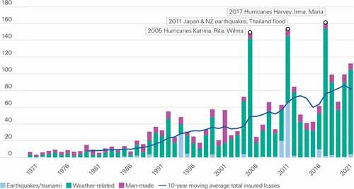Swiss Re Institute (2021) sigma records confirm that insured losses from natural disasters have continued a trend of steady increases of $5-6\mathrm{\%}$ per year over the past few years. Even though insured losses and claims payments have increased significantly over the years, the global property protection gap in disaster risk has steadily widened over the past half century. For instance, the previous 10 years’ economic losses averaged USD 226 billion per year, but only USD 86 billion were covered by insurance, as seen in Figure 1. This illustrates the large gap between the total economic loss and the insurance coverage for disaster risks.

Figure 1. Insured losses since 1970 (USD billion in 2021 prices). Source: .swiss Re Institute (2021)

A better understanding of the factors contributing to underinsurance of risk, particularly in residential property insurance, can narrow the insurance protection gap. Underinsurance can be explained by a variety of factors, such as perceptions of risk, insurance knowledge, affordability, reliance on government post-disaster relief, distrust in insurers, and limited access to insurers (Holzheu & Turner, 2018; Kusuma et al., 2019; Mumo & Watt, 2019). In addition, it is imperative to understand the effects of disasters on insurance demand. These trends also highlight the importance of studies that can help build a better understanding of the effects of exposure to disasters. This will in turn help in designing policies to increase insurance uptake and mitigate the impacts of such disasters on the economy and society in general.

It is globally observed that a unique type of market adjustment occurs in the aftermath of a major disaster event (Auffret, 2003; Born & Viscusi, 2006; Froot & O^!Connell, 1999; Mumo & Watt, 2016). This affects both the demand and supply sides of the insurance market. It is widely acknowledged that post-loss experience influences insurance demand decisions, particularly in the insurance market for catastrophe risks; for example, in California, prior to the 1989 San Francisco earthquake, 34% of people considered earthquake insurance an unimportant undertaking. However, after the earthquake, only 5 percent held this opinion. Similarly, the occurrence of an earthquake increased insurance demand, with 11% of previously uninsured individuals subscribing to an insurance contract (Kunreuther, 1996). Theory and empirical analysis of the insurance markets suggests that riskier and more uncertain markets are typically associated with an increase in insurance demand. According to Ranger and Surminski (2013), this will continue at least until some local threshold is reached where insurance affordability is jeopardized. For instance, Born and Viscusi (2006) explain how premiums for catastrophe risk insurance typically increase dramatically when insurance and reinsurance firms suffer significant loss claims after a natural disaster. The experience with loss events also influences insurance demand behaviour, as numerous other studies have demonstrated. Several studies have shown that higher prior flood damage increases insurance demand (Atreya et al., 2015; Gallagher, 2014; Kousky & Michel-Kerjan, 2017; Turner et al., 2014). A study by Browne and Hoyt (2000) shows that flood insurance purchases are highly correlated with flood losses in the same region previously affected by floods. This insurance demand behaviour is further explained by Cameron and Shah (2012), who find that individuals who have recently experienced a disaster loss report higher probabilities of catastrophic events in the subsequent years. Gallagher (2014) examines the National Flood Insurance Program (NFIP) take-up in communities across the entire United States, grouping many types of flood disasters. In his experiment, he finds an increase in take-up rates after floods, which is consistent with a Bayesian learning model that incorporates forgetting. A study by Kousky and Michel-Kerjan (2017) confirms that insurance purchase is linked to perceptions of disaster likelihood and damage, and that these perceptions are based on a Bayesian process in which individuals update beliefs from past experience. However, disaster experience is only one of many factors that may influence insurance demand following a loss event (Bao et al., 2021; Kousky, 2011; Robinson & Botzen, 2019).

The focus of this paper is to examine the effects generated by disaster experience (post-loss) from an insurance demand-side standpoint and deduce a plausible reason why insurance demand for residential property may change after a catastrophic event. In this study, we hypothesized that regular exposure to disasters would spur measures for prevention and thereby drive up insurance demand. The paper aims to demonstrate how agents can maintain or modify insurance demand after the occurrence of a loss or no-loss event based on a two-period intertemporal setting. This is done by an in-depth analysis and discussion of the performance of the intertemporal insurance model that examines insurance demand changes after a loss event experience. First, we examined the insurance demand post-loss using a two-period intertemporal model, and then we analysed how insurance demand is affected by risk aversion in different periods. In our model, we consider how loss experiences and wealth effects affect risk aversion and insurance demand. We infer, based on only our simulation results, that having an accident increases insurance purchases in the next period compared to when there was no accident in the preceding period. The main results of the present study are in harmony with the existing insurance literature that supports a negative income effect on insurance demand. This is a remarkable characterization of insurance demand, one that fits with both standard insurance economic theory and empirical observations from real-world insurance markets. An important aspect of this study that makes it unique is that it examines both how insurance demand changes post-catastrophe and how it can be theoretically modeled via an intertemporal model. This differs fundamentally from existing studies, which mainly rely on laboratory experiments or empirical analysis.

Catastrophic events have a profound impact on society, and in previous studies (Benali & Feki, 2017; Estrada et al., 2015; McAneney et al., 2016), the total economic and insured losses due to these events has increased substantially. In this light, one significant implication of our results is that a better understanding of how insurance demand changes post-loss experience and what kinds of behavioural factors drive these outcomes can help stakeholders (such as insurance companies, agents, governments, and consumers) develop educational programs and strategies to help improve post-loss outcomes for insurance consumers that include adequate coverage both after a loss and following a no-loss event. The rest of this paper is organized as follows: Section 2 presents a review of the link between the past insurance demand models and the present study. Section 3 presents the methodology, with sub-sections on the theory, the analytical framework, and a numerical illustration of the intertemporal model. Section 4 gives a discussion of several findings that can be drawn from the simulation results, and Section 5 concludes the paper.

2. Link between the past insurance demand models and the present study

Previous theories related to insurance demand focus on insurance in isolation using single-period models. These static models assume that there is only one area of uncertainty in the insurance demand analysis. Several pioneering studies (Arrow (1963), Arrow (1965), Dreze (1981), Mossin (1968), Raviv (1979), and Smith (1968)) are credited for enormous contributions to the analysis of insurance demand in a static setting. With such models, the question of the choice of the level of insurance coverage is not a simple one. Mossin (1968) shows that it is not optimal to purchase full insurance when the price of the insurance is not actuarially fair. These classical models of insurance demand as described in a number of studies (Arrow (1965, 1974); Dreze (1981); Mossin (1968)) have an important deficiency arising from their static features. One clear deficiency is that, in single period models, wealth and consumption are presented by exactly the same variable. A second deficiency lies in the fact that these models do not consider the post-loss implication for insurance demand in a multi-period model with updated wealth. Briys et al. (1988); Dionne and Eeckhoudt (1984); Moffet (1975, 1977) and Mayers and Smith (1983) introduced multiple sources of uncertainty in the analysis of the demand for insurance. More specifically, Dionne and Eeckhoudt (1984); Moffet (1975, 1977) provided joint analyses of the relationship between insurance and saving, and Dionne and Eeckhoudt (1984) further provides two alternative conditions under which a separation theorem holds between insurance and savings. Similarly, Mayers and Smith (1983) examined the interrelationship between insurance holdings and other portfolio decisions and found that the combined analysis leads to different predictions about insurance demand. Extending some of the results obtained by these studies and using the notion of prudence as first introduced in (Eeckhoudt & Kimball, 1992; Kimball, 1991) documents a detailed impact of background risk on the optimal coverage.

Building on this new dynamic approach to insurance analyses, Gollier (2003a) examined a simple consumption lifecycle model where the representative consumer faces a sequence of independent risks over his lifetime. The implicit assumption made in this study is that the policyholders must transform (immediately) the retained loss into a corresponding reduction in demand. This assumption implies that utility for wealth, and the attitude towards risk, are constant over time. However, in the real world, people mostly compensate losses to their wealth by reducing their savings or by borrowing money rather than just reducing their demand over several periods. In (Gollier, 2002) it is shown that a time-consistent cooperative multiplicity strategy provokes consumers to be much more risk susceptible than in the static version of the model. Because of time multiplicity, the attitude towards risk on wealth and towards risk on consumption is not the same. Specifically, the aversion to risk on wealth should be smaller than the aversion to risk on consumption. Meyer and Meyer (2004) suggested that a lower degree of risk aversion for wealth in a multi-period setting translates to depressed demand and welfare gains from insurance. Two reasons are given for these results. First, consumers are keen to consume immediately rather than to perfectly smooth their consumption over time, which implies that they do not adopt a perfect dynamic strategy. Second, they usually face cash constraints, and when funds are needed, policyholders cannot withdraw to compensate for the loss, hence they are obliged to absorb incurred losses immediately. Gollier (2003a) concluded that the ability of consumers to self-insure by accumulating wealth induces them to significantly reduce their demand for insurance relative to what the classical model suggests. However, consumers have a positive insurance demand when they have been unlucky enough to incur a sequence of accidents in the recent past, which reduce their accumulated wealth. This observation is consistent with the literature on insurance demand experiments to test availability heuristic role in the judgment of loss probabilities (see, Kousky (2017); Laury et al. (2009)).

The model proposed in this analysis is in close agreement with the model by Cohen et al. (2008) which examines the implications of a model for multi-period demand decisions on the insurance market. Cohen et al. (2008) looked at the optimal insurance demand strategy of a consumer for a three-year period when the consumer faces a risk of loss in each period. Assuming that the estimated probability of incurring a loss is known and these losses in successive periods are independent, they looked at a perfectly competitive insurance market proposing insurance contracts at actuarially fair premiums corresponding to the estimated expected loss. In this case, insurance contracts are subscribed for one period. Therefore, the consumer has to choose an amount of coverage characterised by the indemnity and premium at each period. Their study revealed that an agent is optimistic in the initial period and modifies risk perception with respect to damages occurring or not.

This analysis takes into cognisant the existing different literature results and builds on this to set up a dynamic intertemporal model. However, this is not the first study to do so. Other studies have already considered and extended the analysis of insurance choices within the context of a multi-period setting (Cohen et al. (2008), Cooper and Hayes (1987), Hofman and Peter (2016), Peter (2017), Peter (2020), Schlesinger (2000), and Volkman-Wise (2015)). We notice that most of these studies do not allow agents to transfer wealth between different periods and only consider situations where consumers only differ in their accident probability. When considering the proposed model, there are new contributions to the insurance dynamic aspects. Since there is no consumption decision, the only effect of the first period decision on the second period decision is through wealth, and all of the standard parameters in the second period like the probability of loss, premium price etc. However, if we allow the free choice of the amount of wealth the agents are allowed to keep and/or transfer, then savings and loans would be essentially the same as consumption. Finally, the model provides a unique way to study the effect of; increase in risk aversion on the insurance demand in different periods by analysing how the local risk aversion changes based on the agent’s wealth effects and loss experience, and increase in the premium on the insurance demand in different periods. In general, it is expected that higher premiums result in lower demand, but a two-period intertemporal model incorporating residual wealth should generate interesting constraints on the demand responses. In the end, this paper presents novel contributions beyond the current dynamic framework which only observes that, risk-averse agents benefit not only from period-by-period events insurance, but also from insurance against a bad risk in a loss event and being reclassified into a higher-risk pool with an associated increased in premiums. This is an important extension to the current literature on dynamic insurance models.

3. Methodology

3.1. The theory of the intertemporal model

The underlying research question in this paper is how the demand for insurance changes post-catastrophe, and how to model it theoretically. To address this question, this paper proposes an intertemporal dynamic model which significantly departs from the popular models in the economic theory of insurance but utilises much of the existing literature findings (see, (Cohen et al. (2008), Cooper and Hayes (1987), Schlesinger (2000), and Volkman-Wise (2015))). The intertemporal dynamic model analyses the insurance consumption decision in an intertemporal setting where an agent is allowed to update insurance demand, initial wealth and a host of other risk and consumption decision parameters in the subsequent periods. In the existing results of income’s effect on insurance demand and intertemporal model, insurance can be sought in two sequential periods of time, and at the second period, it is known whether or not a loss event happened in period one. Thus, it is possible to model the demand for insurance in period two conditional upon the loss event happening or not in period one. The model assumes that for the first period and in successive periods the estimated probability of incurring losses are independent. In essence, then, the intertemporal model of insurance is restricted to only two periods, with an identical insurable risk in each period and identical insurance supply characteristics in each period.

In period one, a decision is made on insurance, and then the period one risk is allowed to play out. Any wealth that is not lost as uninsured losses or premium payments in period one is passed to period two. Then, a decision is made on insurance in period two. It should be noted that the period two decision is made with full information on both the amount of insurance contracted in period one and the outcome of the period one contract, that is, if a loss occurs or not. Since the inherited wealth in period two depends upon the insurance decision in period one, it happens that the insurance decision in period two is expressible as a function of the decision in period one. Therefore, in this model, it is easy to consider the comparison between (i) period two insurance conditional upon a loss in period one and conditional upon no loss in period one, and (ii) period two insurance (either with or without loss event in period one) and the period one insurance demand. It turns out that the model is an interesting extension to the standard model of insurance demand based on a single period and thus provides unique contributions to the theory of insurance demand. Lastly, the results of this model provide a natural theoretical way to establish how the demand for insurance is affected by the size of the loss suffered in the previous period, that is the post-loss insurance demand. The pure theoretical results are derived in the next section.

3.2. Analytical framework

Take an intertemporal perspective, with two consecutive periods as described in the preceding section. In this study, the insurance demand strategy of an agent is examined over the course of two consecutive time periods. In each period, a loss can occur, and insurance coverage can be sought in both periods. Assume there exists an insurer willing to offer insurance contracts that provide positive expected profit.¹ Assume the same loss in each period and that the individual faces a risk of loss of amount $L$ at each period. An insurance contract $C_t$, where $t=1,2$ is proposed for one period. Thus, individuals have to make a decision on the choice of the amount of coverage at each period.

Suppose that for each decision (insurance) period, the estimated probability of incurring a loss is $p$ and that losses in the consecutive periods are independent such that

$P\left(\mathrm{l}\mathrm{o}\mathrm{s}\mathrm{s}\mathrm{a}\mathrm{t}\mathrm{p}\mathrm{e}\mathrm{r}\mathrm{i}\mathrm{o}\mathrm{d}t|\mathrm{l}\mathrm{o}\mathrm{s}\mathrm{s}\mathrm{i}\mathrm{n}\mathrm{p}\mathrm{e}\mathrm{r}\mathrm{i}\mathrm{o}\mathrm{d}t-1\right)=p.$

The outcome of the period one, a situation which is governed by chance, will impact upon the choice to be made in period two. In the same way, the choice made in period one will impact upon the choice made in period two. For instance, in a simple two-dimensional loss situation, in period one a level of insurance coverage $C_1$ is purchased against a loss amount $L$ that happens with probability $p$. If $C_1<L$, that is, partial coverage was purchased, and if the loss happens, then in period two, wealth is lower than it would otherwise have been by the amount of uninsured losses. This will impact upon the decision made in period two. Thus, in period two, the optimal insurance choice, $C_2$, will be a function of (i) the size of loss in period one (at this point, either loss or no loss), (ii) the amount of coverage in period one, and (iii) all the standard parameters in period two. The size of period one’s loss and the level of period one’s coverage will impact upon the level of initial wealth in period two.

It is also assumed that $w_2^i$ denotes the amount of initial wealth in period one, such that; $w_2^1$ is the level of initial period two wealth conditional upon a loss occurring in period one, and $w_2^2$ is the level of initial period two wealth conditional upon no loss occurring in period one. In both periods, wealth is simply the residual wealth from the prior period (net of premium and loss) plus an intertemporal static wage. Insurance is priced linearly, such that an indemnity of $C$ costs $qC$, where $p<q<1$ . The model also introduces an intertemporal preference parameter $\beta$, which is used to measure period two utility in period one utility units.

Now, the consumer’s problem is to choose $C_1$ to maximise the function (1)

$p\left[u\left(w_1-L+C_1(1-q)\right)+\beta \left(pu\left(w_2^1-L+C_2^1(1-q)\right)+(1-p)u\left(w_2^1-q{C}_2^1\right)\right)\right]+$

(1) $(1-p)\left[u\left(w_1-q{C}_1\right)+\beta \left(pu\left(w_2^2-L+C_2^2(1-q)\right)+(1-p)u\left(w_2^2-q{C}_2^2\right)\right)\right],$(1)

where $C_2^i$ maximises

(2) $pu\left(w_2^i-L+C_2^i(1-q)\right)+(1-p)u\left(w_2^i-q{C}_2^i\right).$(2)

Since $w_2^i$ will be a function of $C_1$ for $i=1,2$, this is a problem that needs to be solved recursively using backward induction. Starting then with the two optimisation problems in period two, this gives optimal choice functions $C_2^i(C_2)$. If a loss in period one leads to greater insurance in period two than if no loss happened in period one, then $C_2^1(C_1)>C_2^2(C_1)$. Moreover, if a loss in period one leads to more insurance in period two than what was purchased in period one, then it would see that $C_2^1(C_1)>C_1$.

Observation 1. If the consumer is only partially insured in period one, and a loss event does happen, then initial wealth in period two would be lower by the amount of uninsured loss. So, by under-insuring, the consumer causes a larger decrease in period two wealth when a loss happens in period one, but a higher period two wealth if a loss does not happen in period one (since the period one premium would be lower).

Standard Result: Under decreasing absolute risk aversion (DARA), Observation 1 would also imply a greater demand for coverage in period two. But this is conditional on a loss happening in period one, and partial coverage.

As an example, we use $u(x)=\frac{x^{1-R}-1}{1-R}$, which is constant relative risk aversion (CRRA), and for which $u^{\prime }(x)=x^{-R}$. Starting with the period two choices; we need to choose $C_2^i$ to maximise expression (2).

The first-order condition is expressed in equation (3)(3) $={\left(\frac{w_2^i-q{C}_2^i}{w_2^i-L+C_2^i(1-q)}\right)}^{-R}.$(3)

$\frac{p(1-q)}{q(1-p)}=u(w_2^i-q{C}_2^i)u^{\prime }(w_2^i-L+C_2^i(1-q))$

$=\frac{{(w_2^i-q{C}_2^i)}^{-R}}{{(w_2^i-L+C_2^i(1-q))}^{-R}}$

(3) $={\left(\frac{w_2^i-q{C}_2^i}{w_2^i-L+C_2^i(1-q)}\right)}^{-R}.$(3)

Thus, in this case, we get the expression presented in equation (4)(4) $C_2^i=\frac{w_2^i-{\left(\frac{p(1-q)}{q(1-p)}\right)}^{-\frac{1}{R}}(w_2^i-L)}{{\left(\frac{p(1-q)}{q(1-p)}\right)}^{-\frac{1}{R}}(1-q)+q}.$(4)

${\left(\frac{p(1-q)}{q(1-p)}\right)}^{-\frac{1}{R}}=\frac{w_2^i-q{C}_2^i}{w_2^i-L+C_2^i(1-q)}$

$\left(w_2^i-L+C_2^i(1-q)\right){\left(\frac{p(1-q)}{q(1-p)}\right)}^{-\frac{1}{R}}=w_2^i-q{C}_2^i$

${\left(\frac{p(1-q)}{q(1-p)}\right)}^{-\frac{1}{R}}{C}_2^i(1-q)+q{C}_2^i=w_2^i-{\left(\frac{p(1-q)}{q(1-p)}\right)}^{-\frac{1}{R}}(w_2^i-L)$

$C_2^i\left[{\left(\frac{p(1-q)}{q(1-p)}\right)}^{-\frac{1}{R}}(1-q)+q\right]=w_2^i-{\left(\frac{p(1-q)}{q(1-p)}\right)}^{-\frac{1}{R}}(w_2^i-L)$

(4) $C_2^i=\frac{w_2^i-{\left(\frac{p(1-q)}{q(1-p)}\right)}^{-\frac{1}{R}}(w_2^i-L)}{{\left(\frac{p(1-q)}{q(1-p)}\right)}^{-\frac{1}{R}}(1-q)+q}.$(4)

If we set ${\left(\frac{p(1-q)}{q(1-p)}\right)}^{-\frac{1}{R}}\equiv k$, then the optimal insurance purchase in period two is expressed as shown in equation (5)(5) $C_2^i=\frac{w_2^i-k(w_2^i-L)}{k(1-q)+q}.$(5) ;

(5) $C_2^i=\frac{w_2^i-k(w_2^i-L)}{k(1-q)+q}.$(5)

It can be noted that the only difference between the two options is the size of initial wealth, $w_2^i$. Thus, we now have equation (6)(6) $\frac{\mathrm{\partial }{C}_2^i}{\mathrm{\partial }{w}_2^i}=\frac{1-k}{k(1-q)+q}.$(6) ;

(6) $\frac{\mathrm{\partial }{C}_2^i}{\mathrm{\partial }{w}_2^i}=\frac{1-k}{k(1-q)+q}.$(6)

Since the denominator of equation (6)(6) $\frac{\mathrm{\partial }{C}_2^i}{\mathrm{\partial }{w}_2^i}=\frac{1-k}{k(1-q)+q}.$(6) is positive, the effect of larger initial wealth upon the optimal insurance purchase is positive if $k<1$, and negative if $k>1$. We note that $k>1$ if $p(1-q)<q(1-p)$, in which case $p<q$. This is the condition for positive insurer’s profits, so it should be assumed to be so, in which case the greater $C_2^i$ is, the smaller $w_2^i$ is. Assuming partial insurance in period one, it is expected that $w_2^1<w_2^2$, that is, smaller initial period two wealth if a loss is suffered in period one than if not. In this case, then, the period two insurance purchase is greater after a period one loss has happened than when a period one loss did not happen.

Figure 2 and 3 presents a three dimensional plot of the ratios of premium loading factor to the loss probability. In this case, the loading factor indicates that insurance is priced linearly subject to the condition that $p<q<1$.

Figure 2. Three dimensional plot of the ratios of premium loading factor to the loss probability.

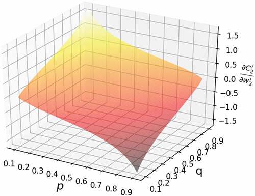
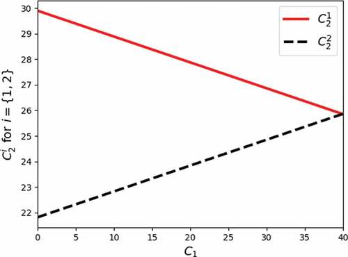
Figure 3. Comparison of loss ($C_2^1$) and no loss ($C_2^2$) against $C_1$.

The indirect utility function for period two can thus be written as in equation (7)(7) $=Eu\left(w_2^i\right)$(7) ;

$pu\left(w_2^i-L+C_2^i(1-q)\right)+(1-p)u\left(w_2^i-q{C}_2^i\right)=p\frac{{\left(w_2^i-L+C_2^i(1-q)\right)}^{1-R}-1}{1-R}$

$+(1-p)\frac{{(w_2^i-q{C}_2^i)}^{1-R}-1}{1-R}$

(7) $=Eu\left(w_2^i\right)$(7)

In order to continue, a proposition is made on how the period one outcome affects period two initial wealth.

Proposition 1. Let $w$ be a constant amount indicating the intertemporal wage. If savings are rewarded with an interest rate of zero and that there is no consumption outside of insurance in period one, then with the assumption that wealth is simply the residual wealth from the prior period plus an intertemporal static wage, the proposition now leads to equations (8)(8) $w_2^1=w_1+C_1(1-q)-L+w,$(8) and (9(9) $w_2^2=w_1-q{C}_1+w.$(9) );

(8) $w_2^1=w_1+C_1(1-q)-L+w,$(8)

(9) $w_2^2=w_1-q{C}_1+w.$(9)

When the period one insurance choice is made, the consumer now maximises the expected utility function as in expression (10);

(10) $V=p\left[u\left(w_1-L+C_1(1-q)+\beta Eu\left(w_2^1\right)\right)\right]+(1-p)\left[u\left(w_1-q{C}_1\right)+\beta Eu\left(w_2^2\right)\right]$(10)

The first-order condition associated with equation (10)(10) $V=p\left[u\left(w_1-L+C_1(1-q)+\beta Eu\left(w_2^1\right)\right)\right]+(1-p)\left[u\left(w_1-q{C}_1\right)+\beta Eu\left(w_2^2\right)\right]$(10) can be simplified as given in equation (11)(11) $+(1-p)\left(u^{\prime }(w_1-q{C}_1)(-q)+\beta \frac{\mathrm{\partial }Eu(w_2^2)}{\mathrm{\partial }{w}_2^2}\frac{\mathrm{\partial }{w}_2^2}{d{C}_1}=0\right)$(11) ;

$p\left(u^{\prime }\left(w_1-L+C_1(1-q)\right)(1-q)+\beta \frac{\mathrm{\partial }Eu(w_2^1)}{\mathrm{\partial }{w}_2^1}\frac{\mathrm{\partial }{w}_2^1}{d{C}_1}\right)$

(11) $+(1-p)\left(u^{\prime }(w_1-q{C}_1)(-q)+\beta \frac{\mathrm{\partial }Eu(w_2^2)}{\mathrm{\partial }{w}_2^2}\frac{\mathrm{\partial }{w}_2^2}{d{C}_1}=0\right)$(11)

Using the specific utility function $u(x)$ and its derivative, the expression $V$ becomes $V_1$ given by,

(12) $0.9!\begin{array}{c}{V}_1=p\left(\frac{{(w_1-L+C_1(1-q))}^{1-R}-1}{1-R}+\beta \left(\frac{{(w_2^1-L+C_2^1(1-q))}^{1-R}-1}{1-R}+(1-p)\frac{{(w_2^1-q{C}_1)}^{1-R}-1}{1-R}\right)\right)\\ +(1-p)\left(\frac{{(w_1-q{C}_1)}^{1-R}-1}{1-R}+\beta \left(p\frac{{(w_2^1-L+C_2^2(1-q))}^{1-R}-1}{1-R}+(1-p)\frac{{(w_2^2-q{C}_2^2)}^{1-R}-1}{1-R}\right)\right)\end{array}$(12)

and the equation for first-order condition for minimisation becomes

(13) $\begin{array}{c}p\left({(w_1-L+C_1(1-q))}^{-R}(1-q)+\beta \left(p{(w_2^1-L+C_2^1(1-q))}^{-R}\left(1+(1-q)\frac{\mathrm{\partial }{C}_2^1}{\mathrm{\partial }{w}_2^1}\right)\right.\right.\\ +\left.\left.(1-p)(w_2^1-q{C}_2^1{)}^{-R}\left(1-q\frac{\mathrm{\partial }{C}_2^1}{\mathrm{\partial }{w}_2^1}\right)\right)(1-q)\right)+(1-p)\left({(w_1-q{C}_1)}^{-R}(-q)\right.\\ +\beta \left(p{(w_2^1-L+C_2^2(1-q))}^{-R}\left(1+(1-q)\frac{\mathrm{\partial }{C}_2^2}{\mathrm{\partial }{w}_2^2}\right)\right.+\left.(1-p)(w_2^2-q{C}_2^2{)}^{-R}\left(1-q\frac{\mathrm{\partial }{C}_2^2}{\mathrm{\partial }{w}_2^2}\right)\right)=0,\end{array}$(13)

with $C_2^i=\frac{w_2^i-k(w_2^i-L)}{k(1-q)+q}$ such that $C_2^1=\frac{w_2^1-k(w_2^1-L)}{k(1-q)+q}$, $C_2^2=\frac{w_2^2-k(w_2^2-L)}{k(1-q)+q}$ and $k={\left(\frac{p(1-q)}{q(1-p)}\right)}^{-\frac{1}{R}}$.

On substituting the terms of $w_2^1$ and $w_2^2$ into expressions for $C_2^i$, we obtain

(14) $\begin{array}{cc}{C}_2^1& =\frac{(w_1+C_1(1-q)-L+w)-{\left(\frac{p(1-q)}{q(1-p)}\right)}^{-\frac{1}{R}}((w_1+C_1(1-q)-L+w)-L)}{{\left(\frac{p(1-q)}{q(1-p)}\right)}^{-\frac{1}{R}}(1-q)+q}\\ C_2^2& =\frac{(w_1-q{C}_1+w)-{\left(\frac{p(1-q)}{q(1-p)}\right)}^{-\frac{1}{R}}(w_1-q{C}_1+w-L)}{{\left(\frac{p(1-q)}{q(1-p)}\right)}^{-\frac{1}{R}}(1-q)+q}.\end{array}$(14)

We observe that, equations (10)(10) $V=p\left[u\left(w_1-L+C_1(1-q)+\beta Eu\left(w_2^1\right)\right)\right]+(1-p)\left[u\left(w_1-q{C}_1\right)+\beta Eu\left(w_2^2\right)\right]$(10) -(14(14) $\begin{array}{cc}{C}_2^1& =\frac{(w_1+C_1(1-q)-L+w)-{\left(\frac{p(1-q)}{q(1-p)}\right)}^{-\frac{1}{R}}((w_1+C_1(1-q)-L+w)-L)}{{\left(\frac{p(1-q)}{q(1-p)}\right)}^{-\frac{1}{R}}(1-q)+q}\\ C_2^2& =\frac{(w_1-q{C}_1+w)-{\left(\frac{p(1-q)}{q(1-p)}\right)}^{-\frac{1}{R}}(w_1-q{C}_1+w-L)}{{\left(\frac{p(1-q)}{q(1-p)}\right)}^{-\frac{1}{R}}(1-q)+q}.\end{array}$(14) ) are as a result of proposition 1 and its defining conditions (8) and (9). In equation (14)(14) $\begin{array}{cc}{C}_2^1& =\frac{(w_1+C_1(1-q)-L+w)-{\left(\frac{p(1-q)}{q(1-p)}\right)}^{-\frac{1}{R}}((w_1+C_1(1-q)-L+w)-L)}{{\left(\frac{p(1-q)}{q(1-p)}\right)}^{-\frac{1}{R}}(1-q)+q}\\ C_2^2& =\frac{(w_1-q{C}_1+w)-{\left(\frac{p(1-q)}{q(1-p)}\right)}^{-\frac{1}{R}}(w_1-q{C}_1+w-L)}{{\left(\frac{p(1-q)}{q(1-p)}\right)}^{-\frac{1}{R}}(1-q)+q}.\end{array}$(14) , we can see that the loss in period one leads to greater insurance in period two than if no loss happened in period one, which means $C_2^1(C_1)>C_2^2(C_1)$. How much larger is $C_2^1$ and $C_2^2$ will depend on the underlying utility curvature parameter $R$. We observe that when $R$ is increased $k$ approaches one for $p<q$: More precisely $R$ grows without bound ($R\to \mathrm{\infty }$) as $k$ approaches $1$ and in this case $C_2^1$ and $C_2^2$ approach $L$ and the difference between $C_2^1$ and $C_2^2$ approaches zero.

3.3. Numerical illustration of the intertemporal model

In this section, we demonstrate how insurance demand varies pre—and post-loss. The insurance scenario described by the intertemporal framework model is simulated for the set of selected hypothetical values and results are shown in the following scenario.

We now consider nominal values for the parameters defined in section 3.2 as presented in Table 1.

Table 1. Nominal values of the parameter

Parameter	$w_1$	$w$	$L$	$p$	$q$	$R$	$\beta$
Nominal value	$100$	$10$	$40$	$0.4$	$0.5$	$2$	$0.9$

Then;

$C_2^1=\frac{\left(100+C_1(1-0.5)-40+10\right)-\left({\left(\frac{0.4(1-0.5)}{0.5(1-0.4)}\right)}^{-\frac{1}{2}}\right)\left((100+C_1(1-0.5)-40+10)-40\right)}{\left({\left(\frac{0.4(1-0.5)}{0.5(1-0.4)}\right)}^{-\frac{1}{2}}\right)(1-0.5)+0.5}$

$=29.898-0.10102C_1.$

$C_2^2=\frac{100-0.5C_1+10-\left({\left(\frac{0.4(1-0.5)}{0.5(1-0.4)}\right)}^{-\frac{1}{2}}\right)(100-0.5C_1+10-40)}{\left({\left(\frac{0.4(1-0.5)}{0.5(1-0.4)}\right)}^{-\frac{1}{2}}\right)(1-0.5)+0.5}$

$=0.10102C_1+\mathrm{21.816.}$

Since $C_2^i$ depends on uncovered loss $C_1$, the illustration shows a comparison of loss ($C_2^1$) and no loss ($C_2^2$) with and without intertemporal consideration respectively.

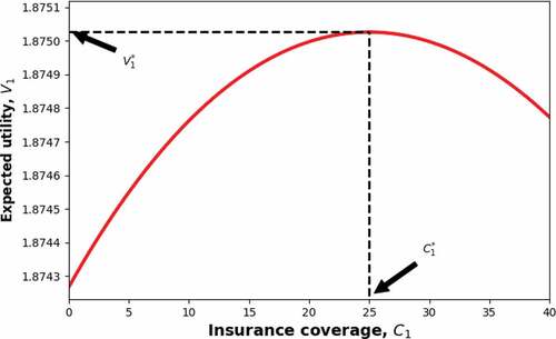
We now solve for the optimal value(s) of $C_1$. Using the parameter values in Table 1, the expression for $V_1$ as a function of insurance coverage with intertemporal consideration is plotted on Figure 4

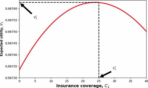
Figure 4. Optimal insurance coverage with intertemporal consideration. The optimal value is at $C_1^{\ast }\approx 24.992$, at which point the greatest expected utility is valued at $V_1^{\ast }\approx 1.8750$. (The interval of $C_1$ over which the plotting is done was subdivided $1,000,000$ times to ensure that an accurate value of the index of $C_1$ is used to obtain the maximum value of $V_1$).

We now compare the optimal values of $V_1$ (the case with intertemporal consideration) to the optimal values of $V_2$ (for the case without intertemporal consideration) where,

(15) $V_2=0.4\left(\frac{{(100-40+C(1-0.5))}^{1-R}-1}{1-R}\right)+(1-0.4)\left(\frac{{(100-0.5C)}^{1-R}-1}{1-R}\right).$(15)

The graph of $V_2$ is indicated in Figure 5 with the greatest utility valued at $V_2^{\ast }\approx 0.98763$ which is obtained at the optimal coverage of $C_1^{\ast }\approx 24.992$.

Figure 5. Optimal insurance coverage with intertemporal consideration. The optimal value is at $C_1^{\ast }\approx 24.992$, at which point the greatest expected utility is valued at $V_2^{\ast }\approx 0.98763$.

4. Results and discussion

The properties of this model have been demonstrated both analytically and numerically that $C_2^1(C_1)>C_2^2(C_1)$ and how $C_2^i$ and relates to $C_i$; this is also supported by the assumption of a CRRA utility function. Results of the numerical simulation are indicated in Figures 4 and 5. It’s observed that the optimal insurance demand with or without intertemporal consideration is at approximately $24.992$. This is partly due to the lack of existence of a consumption smoothing mechanism. Future studies can explore the effects of savings as a consumption smoothing mechanism, and then extend the intertemporal model into more periods to determine what happens in general to the trend of insurance purchases in the provision of coverage for both catastrophe and non-catastrophic losses.

Based on our derived model (for this example), taking into account the intertemporal nature increases insurance demand. This can be illustrated by $C_2^1$ and $C_2^2$

$C_2^1=29.898-0.10102\times 24.992=27.373$

$C_2^2=0.10102\times 24.992+21.816=\mathrm{24.341.}$

Results of the numerical simulation in this analysis indicate that insurance demand increases immediately after the loss event. In fact, it can be seen that the insurance demand after loss increases by $9.5$ percent (that is, from $24.992$ to $27.373$), and the demand if no loss falls by $2.6$ percent (that is, from $24.992$ to $24.341$). Based only upon our simulation results, we infer that the experience of having an accident increasing insurance purchases in the next period relative to insurance purchases when in the immediately prior period there was no accident. This is in line with standard insurance economic theory on insurance demand and empirical observations from real-world insurance markets, and also supported by empirical work by Browne and Hoyt (2000) and Cameron and Shah (2012).

short-legendGraph 1.

short-legendGraph 2.

The present model only looked into the wealth in the second period with no consumption, that is, simply the wealth of the first period minus loss plus income. However, there is still utility derived from this wealth, but this model is restricted to solve insurance demand in an intertemporal setting in absence of consumption choices. In any case, this utility cannot be consumption as that would reduce the transferred wealth, but if we allow the free choice of the amount of wealth the agents are allowed to keep and/or transfer, then savings and loans will be essentially the same as consumption. However, since the wealth is evaluated through two utility functions, it is ambiguous how the results translate to known comparative statics results. The present model acknowledge the assumptions that no consumption and that the wealth in second period is the inherited wealth from the prior period (net of premium and loss) plus an intertemporal static wage are limiting and that there is a need for further theory to model explicitly the utility derived from the wealth in the second period, further research is needed on this question. Additional research is also needed on the effect of consumption decision and corresponding methodology to solve the associated bivariate optimisation problem.

5. Conclusions

The focus of this paper was on the effects of post-loss experience from an insurance demand-side perspective. Our main objective was to develop a theoretical model that helped to explain how insurance demand is affected by the size of the loss suffered in the previous period, that is, the post-loss insurance demand. First, we examined the insurance demand post-loss using a two-period intertemporal model, and then we analysed how insurance demand is affected by risk aversion in different periods. The model shows how loss experiences and wealth effects affect risk aversion and changes in insurance demand. Based on only our simulation result, we infer that having an accident leads to an increase in insurance purchases in the next period relative to insurance purchases when in the immediately prior period there was no accident. The main results of the present study are in harmony with the existing insurance literature that supports a negative income effect on insurance demand. This is a remarkable characterization of insurance demand in line with standard insurance economic theory and empirical observations from real-world insurance markets. One significant implication of our results is that a better understanding of how insurance demand changes post-loss experience and what kinds of behavioural factors drive these outcomes can help stakeholders (such as insurance companies, agents, governments, and consumers) develop educational programs and strategies to help improve post-loss outcomes for insurance consumers that include adequate coverage both after a loss and following a no-loss event.

Finally, note that our proposition of no consumption and that the wealth in the second period is the inherited wealth (net of premium and loss) plus an intertemporal static wage is limiting. This limitation offers an interesting area of exploration. More studies are thus encouraged to model explicitly the utility derived from the wealth in the second period. In addition, further research is needed into the effects of consumption decisions and how to solve the bivariate optimization problem that results.

Disclosure statement

No potential conflict of interest was reported by the author(s).

Additional information

Funding

R. K. Mumo acknowledges the financial support from BIUST under grant number Botswana International University of Science and Technology <#AWARD-ID;>R00132</#AWARD-ID;></#AWARD-ID;>.

Notes on contributors

Richard Mumo

Richard Mumo is a Lecturer in Financial Mathematics at Botswana International University of Technology. His research interests focuses on the economics of natural disaster risk management, insurance product pricing, actuarial science and financial modelling, climate risk and adaptation, and climate finance.

John Boscoh H. Njagaraha

John Boscoh H. Njagaraha is a Lecturer in Mathematical Modelling at Botswana International University of Technology. His research focuses on applied mathematics in general, with particular emphasis on the applications of dynamical systems to infectious disease dynamics, substance abuse, and other biological systems.

Mercy K. Kiremu

Mercy K. Kiremu is a Management Accountant at the Waikato District Health Board. She previously worked as a lecturer in accounts and finance at the Western Institute of Technology at Taranaki. Her research interests and areas of expertise include climate finance, climate risk, financial risk, governance, and assurance.

Richard Watt

Richard Watt is a Professor of Economics at the University of Canterbury. His research focuses on applied microeconomics generally, with particular emphasis on the economic theory of risk bearing and the economics of copyright.

Notes

1. If the contracts were actuarially fair, the insured would only purchase full coverage always. We need, therefore, that the contracts be actuarially unfair, or in other words, that they offer positive expected profit to the insurer.

References

- Arrow, K. J. (1963). Uncertainty and the welfare economics of medical care. The American Economic Review, 53(5), 941–18.
- Arrow, K. J. (1965). Aspects of the theory of risk-bearing. Yrjö Jahnssonin Säätiö, Helsinki.
- Arrow, K. J. (1974). Optimal insurance and generalized deductibles. Scandinavian Actuarial Journal, 1974(1), 1–42. https://doi.org/10.1080/03461238.1974.10408659
- Atreya, A., Ferreira, S., & Michel-Kerjan, E. (2015). What drives households to buy flood insurance? New evidence from Georgia. Ecological Economics, 117, 153–161. https://doi.org/10.1016/j.ecolecon.2015.06.024
- Auffret, P. (2003). High consumption volatility: The impact of natural disasters? World Bank Policy Research Working Paper, No. 2962. https://doi.org/10.1596/1813-9450-2962
- Bao, X., Zhang, F., Deng, X., & Xu, D. (2021). Can trust motivate farmers to purchase natural disaster insurance? Evidence from earthquake-stricken areas of sichuan, China. Agriculture, 11(8), 783. https://doi.org/10.3390/agriculture11080783
- Benali, N., & Feki, R. (2017). The impact of natural disasters on insurers’ profitability: Evidence from property/casualty insurance company in United States. Research in International Business and Finance, 42, 1394–1400. https://doi.org/10.1016/j.ribaf.2017.07.078
- Born, P., & Viscusi, W. K. (2006). The catastrophic effects of natural disasters on insurance markets. Journal of Risk and Uncertainty, 33(1–2), 55–72. https://doi.org/10.1007/s11166-006-0171-z
- Briys, E., Kahane, Y., & Kroll, Y. (1988). Voluntary insurance coverage, compulsory insurance, and risky-riskless portfolio opportunities. Journal of Risk and Insurance, 55(4), 713–722. https://doi.org/10.2307/253147
- Browne, M. J., & Hoyt, R. E. (2000). The demand for flood insurance. Empirical Evidence.Journal of Risk and Uncertainty, 20(3), 291–306. https://doi.org/10.1023/A:1007823631497
- Cameron, L., & Shah, M. (2012). ‘Risk-taking behavior in the wake of natural disasters’. IZA Discussion Papers, No. 6756, Institute for the Study of Labor (IZA).
- Cohen, M., Etner, J., & Jeleva, M. (2008). Dynamic decision making when risk perception depends on past experience. Theory and Decision, 64(2–3), 173–192. https://doi.org/10.1007/s11238-007-9061-3
- Cooper, R., & Hayes, B. (1987). Multi-period insurance contracts. International Journal of Industrial Organization, 5(2), 221–231. https://doi.org/10.1016/S0167-7187(87)80020-6
- Dionne, G., & Eeckhoudt, L. (1984). Insurance and saving: Some further results. Insurance, Mathematics & Economics, 3, 101–110. https://doi.org/10.1016/0167-6687(84)90048-9
- Dreze, J. H. (1981). Inferring risk tolerance from deductibles in insurance contracts. Geneva Papers on Risk and Insurance, 6(20), 48–52. https://doi.org/10.1057/gpp.1981.17
- Eeckhoudt, L., & Kimball, M., (1992). Background risk, prudence, and the demand for insurance, in Contributions to insurance economics, G. Dionne Ed., Springer Netherlands. 239–254.
- Estrada, F., Botzen, W. W., & Tol, R. S. (2015). Economic losses from US hurricanes consistent with an influence from climate change. Nature Geoscience, 8(11), 880–884. https://doi.org/10.1038/ngeo2560
- Froot, K. A., & O’Connell, P. G. (1999). The pricing of US catastrophe reinsurance, in The Financing of Catastrophe Risk Froot, K. A, Ed. University of Chicago Press. 195–227.
- Gallagher, J. (2014). Learning about an infrequent event: Evidence from flood insurance take-up in the United States. American Economic Journal. Applied Economics, 6(3), 206–233.
- Gollier, C. (2002). Time diversification, liquidity constraints, and decreasing aversion to risk on wealth. Journal of Monetary Economics, 49(7), 1439–1459. https://doi.org/10.1016/S0304-3932(02)00173-3
- Gollier, C. (2003a). To insure or not to insure?: An insurance puzzle. The Geneva Papers on Risk and Insurance Theory, 28(1), 5–24. https://doi.org/10.1023/A:1022112430242
- Gollier, C. (2003b). To insure or not to insure?: An insurance puzzle. GENEVA Papers on Risk and Insurance-Theory, 28(1), 5–24. https://doi.org/10.1023/A:1022112430242
- Hofman, A., & Peter, R. (2016). Self-insurance, self-protection, and saving: On consumption smoothing and risk management. Journal of Risk and Insurance, 83(3), 719–734. https://doi.org/10.1111/jori.12060
- Holzheu, T., & Turner, G. (2018). The natural catastrophe protection gap: Measurement, root causes and ways of addressing underinsurance for extreme events. The Geneva Papers on Risk and Insurance-Issues and Practice, 43(1), 37–71. https://doi.org/10.1057/s41288-017-0075-y
- Kimball, M. S. (1991). Precautionary motives for holding assets, NBER Working Paper No. 3586. National Bureau of Economic Research, Cambridge.
- Kousky, C. (2011). Understanding the demand for flood insurance. Natural Hazards Review, 12(2), 96–110. https://doi.org/10.1061/(ASCE)NH.1527-6996.0000025
- Kousky, C. (2017). Disasters as learning experiences or disasters as policy opportunities? Examining flood insurance purchases after hurricanes. Risk Analysis, 37(3), 517–530. https://doi.org/10.1111/risa.12646
- Kousky, C., & Michel-Kerjan, E. (2017). Examining flood insurance claims in the United States: Six key findings. Journal of Risk and Insurance, 84(3), 819–850. https://doi.org/10.1111/jori.12106
- Kunreuther, H. (1996). Mitigating disaster losses through insurance. Journal of Risk and Uncertainty, 12(2–3), 171–187. https://doi.org/10.1007/BF00055792
- Kusuma, A., Nguyen, C., & Noy, I. (2019). Insurance for catastrophes: Why are natural hazards underinsured, and does it matter? In Advances in spatial and economic modeling of disaster impacts (pp. 43–70). Springer.
- Laury, S. K., McInnes, M. M., & Swarthout, J. T. (2009). Insurance decisions for low-probability losses. Journal of Risk and Uncertainty, 39(1), 17–44. https://doi.org/10.1007/s11166-009-9072-2
- Mayers, D., & Smith, C. W., Jr. (1983). The interdependence of individual portfolio decisions and the demand for insurance. Journal of Political Economy, 91(2), 304–311. https://doi.org/10.1086/261145
- McAneney, J., McAneney, D., Musulin, R., Walker, G., & Crompton, R. (2016). Government-sponsored natural disaster insurance pools: A view from down-under. International Journal of Disaster Risk Reduction, 15, 1–9. https://doi.org/10.1016/j.ijdrr.2015.11.004
- Meyer, D., & Meyer, J. (2004). A more reasonable model of insurance demand, in assets, beliefs, and equilibria in economic dynamics. In C. D. Aliprantis, K. J. Arrow, P. Hammond, F. Kubler, H. M. Wu, & N. C. Yannelis (Eds.), Essays in honor of mordecai kurz, studies in economic theory (Vol. 18, pp. 733–742). Springer-Verlag.
- Moffet, D. (1975). Risk Bearing and Consumption Theory. ASTIN Bulletin: The Journal of the IAA, 8(3), 342–358. https://doi.org/10.1017/S0515036100011272
- Moffet, D. (1977). Optimal deductible and consumption theory. Journal of Risk and Insurance, 44(4), 669–683. https://doi.org/10.2307/251727
- Mossin, J. (1968). Aspects of rational insurance purchasing. The Journal of Political Economy, 76(4), 553–568. https://doi.org/10.1086/259427
- Mumo, R., & Watt, R. (2016). The dual insurance model and its implications for insurance demand and supply post-Christchurch earthquakes in New Zealand. Insurance and Risk Management, 83(3–4), 135–167.
- Mumo, R., & Watt, R. (2019). Residential insurance market responses after earthquake: A survey of Christchurch dwellers. International Journal of Disaster Risk Reduction, 40, 101166. https://doi.org/10.1016/j.ijdrr.2019.101166
- Peter, R. (2017). Optimal self-protection in two periods: On the role of endogenous saving. Journal of Economic Behavior & Organization, 137, 19–36. https://doi.org/10.16/j.jebo.2017.01.017
- Peter, R. (2020). Who should exert more effort? risk aversion, downside risk aversion and optimal prevention. Economic Theory, 71(4), 1259–1281. https://doi.org/10.1007/s00199-020-01282-0
- Ranger, N., & Surminski, S. (2013). A preliminary assessment of the impact of climate change on non-life insurance demand in the BRICS economies. International Journal of Disaster Risk Reduction, 3, 14–30. https://doi.org/10.1016/j.ijdrr.2012.11.004
- Raviv, A Dionne, G. (1979). The design of an optimal insurance policy. American Economic Review, 69(1), 84–96.
- Robinson, P. J., & Botzen, W. W. (2019). Determinants of probability neglect and risk attitudes for disaster risk: An online experimental study of flood insurance demand among homeowners. Risk Analysis, 39(11), 2514–2527. https://doi.org/10.1111/risa.13361
- Schlesinger, H. (2000). The theory of insurance demand. In Handbook of insurance (pp. 131–151). Springer Netherlands.
- Smith, V. L. (1968). Optimal insurance coverage. The Journal of Political Economy, 76(1), 68–77. https://doi.org/10.1086/259382
- Swiss Re Institute (2021). sigma No 1/2021: Natural catastrophes in 2020: secondary perils in the spotlight, but don’t forget primary-peril risks. Retrieved December 20, 2021, from https://www.swissre.com/dam/jcr:ebd39a3b-dc55-4b34-9246-6dd8e5715c8b/sigma-1–2021-en.pdf
- Turner, G., Said, F., & Afzal, U. (2014). Microinsurance demand after a rare flood event: Evidence from a field experiment in Pakistan. The Geneva Papers on Risk and Insurance-Issues and Practice, 39(2), 201–223. https://doi.org/10.1057/gpp.2014.8
- Volkman-Wise, J. (2015). Representativeness and managing catastrophe risk. Journal of Risk and Uncertainty, 51(3), 267–290. https://doi.org/10.1007/s11166-015-9230-7