The bilateral J-curve between Ghana and her key trading partners

Abstract

This study examines the J-Curve phenomenon of a developing country for the case of Ghana and its major trade partners: Switzerland (Swiss) and China. Using quarterly bilateral data from Q1-1995 to Q4-2018 to investigate the impact of currency depreciation on the bilateral trade balance in the short and the long run, it was established that the depreciation of Ghana Cedis in recent years could be considered as a successful policy for the trade balance improvement of Ghana. First, the real depreciation of Ghana Cedis improves Ghana’s trade balance with China and the Swiss after worsening the trade balance in the short run. Second, in the long run, the Ghana trade balance is improved from a real depreciation of Cedis, which formed 3.235 percent and 1.594 percent of Ghana’s total trade share with China and Swiss, respectively. Third, the estimates show evidence of the J-Curve phenomenon only in the cases of China, not for the Swiss. Additionally, the real income of trading partners has a positive and significant effect in the long run, indicating that an increase in the real income of partners has an important role in determining imports from Ghana. However, there is no significant effect on Ghana’s real income on the trade balance. Lastly, the results from diagnostic tests show that the estimated relationships have been stable and reliable over the last 24 years. Consequently, in line with the study results, the authors recommend several policy implications to improve the trade balance in Ghana.

Keywords:

• J-Curve phenomenon
• bilateral trade balance
• real exchange rate
• ARDL approach
• Ghana

JEL Codes:

• F13
• F14
• F31
• B27

PUBLIC INTEREST STATEMENT

Local currency movement is of crucial interest to policymakers and stakeholders owing to its ripple effect in all spheres of the economy. A higher-valued currency makes a nation’s imports relatively affordable and its exports relatively expensive in foreign markets, whiles a lower-valued currency makes a country’s imports more expensive and its exports less expensive in foreign markets. Therefore, a higher exchange rate can be expected to worsen a country’s balance of trade, while a lower exchange rate can be expected to improve it, as argued by the J-curve theory. However, this study, among other studies, shows that an initial worsening of a nation’s trade balance following a depreciation of its currency might not always result in a dramatic gain in the trade balance in the long run. Thus, nations especially developing countries such as Ghana, in this case, should strive for a stable and competitive exchange rate policy anchored on the nation’s trade prowess.

1. Introduction

International trade substantially influences a country’s overall economic growth and development (Dogru et al., 2019). Governments worldwide pursue a variety of economic policies meant to improve trade and economic development. The trade balance is a key indicator in evaluating a country’s international trade performance. Improving a country’s balance of trade will boost its current account balance and GDP as a whole, and vice versa. Unfortunately, the majority of Sub-Saharan African (SSA) economies have consistently run a trade deficit. This consistent weakening of the current account balance reflects the region’s overall incessant trade deficit. As a result, these economies’ growth and development may be jeopardized. Therefore, a robust export sector is essential in order to keep the trade balance of the SSA in a better position as it has been the pillar of most of the economies in East Asia. Although a spotlight on investment, technological advancement, and innovation are some of the long-term actions to build a robust export sector to curb the dwindling trade balance situation, the exchange rate has been mentioned as one of the most generally used short term mitigating policies to restrict a falling trade balance (Bahmani-Oskooee & Ratha, 2004; Işik et al., 2019; Ongan et al., 2018b, 2017). Particularly for developing nations, it has been implied that exchange rate depreciation is a suitable macroeconomic fundamental policy strategy to support the export sector (Vitale, 2003).

The exchange rate is considered an essential macroeconomic factor that affects other variables in a nation’s a trade and capital flows. In an attempt to push international competitiveness as well as improve the trade balance, devaluation of the national currency is considered an effective measure (Dogru et al., 2019). In theory, the response of export and import volumes to the real exchange rate affects the trade balance. As a result of currency depreciation, while imports will become more expensive, exports will become cheaper in the short term. Nevertheless, the trade balance would be improved in the long-term after the beginning worsening. The reason is that short-term trade in goods is inelastic because it takes time to change consumption patterns and trade contracts (Bahmani-Oskooee & Ratha, 2004); however, the long-term trade balance is expected to improve as consumers adjust to the new prices. This phenomenon is commonly known as the J-Curve phenomenon. Meanwhile, following the Marshall-Lenner condition, the absolute sum of import and export demand elasticities exceeding one will decide the success of the devaluation. Nonetheless, neither theoretical models nor empirical studies on the J-curve effect have produced a conclusive rejoinder (Baum & Caglayan, 2010).

The recent rate of globalization, which has affected the sensitivity of the trade balance to real exchange rates, has fueled the debate even further. A higher degree of vertical specialization and new global supply chains, on the one hand, tend to reduce the responsiveness of trade balance to the movement of the real exchange rate. On the other hand, increased intra-industry trade makes the trade balance more sensitive to changes in real exchange rates (Akosah & Omane-Adjepong, 2017). The complementarity between imports and exports is enhanced by vertical specialization and a global supply chain. However, the relative importance of these two effects differs from country to country due to differences in the degree of substitutability of imported and exported goods. Countries with low intra-industry trade, for example, are expected to be more sensitive to changes in real exchange rates than those with high intra-industry trade (Kharroubi, 2011). In contrast, imports tend to fall precipitously in a high intra-industry trade country that depreciates its real exchange rate because these countries can more easily provide domestic substitutes for imported goods that have become more expensive (Akosah & Omane-Adjepong, 2017; Kharroubi, 2011). Therefore, the literature suggests that the responsiveness of trade balance to the real exchange rate movement positively relates to intra-industry trade.

Ghana, a developing country with underdeveloped capital markets coupled with supply constraints just like any other SSA country, will need a robust real exchange rate as a viable macroeconomic policy to boost trade balance. Following the financial liberalization initiative powered by the International Monetary Fund (IMF) through the World Bank’s Economic Recovery (ERP) and Structural Adjustment Programs (SAP), Ghana’s exchange rate regime shifted from fixed to floating after 1983. Since then, the exchange rate movement has attracted the great attention of policymakers and researchers as a significant macroeconomic indicator to gauge the entire economy. The Ghanaian economy has been characterized by continual trade imbalances and prevalent currency depreciation over the last three decades. Simultaneously, the domestic currency has remained one of the world’s weakest. In recent years, particularly in 2019, the government committed assiduous efforts such as the introduction of higher denominations of local currency, among other efforts to boost trade, yet the trade balance is still dwindling. These developments have rekindled interest in better understanding the impact of exchange rates on Ghana’s external trade. Despite the growing number of studies on the subject, the actual impact of exchange rates on Ghana’s external trade remains an open and contentious issue.

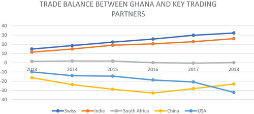
Ghana’s top five export and import partners based on the 2019 data provided by (WITS) World Integrated Trade Solutions (Partner share (%)) are China, 16.75%; Switzerland, 14.71%; India, 14.19%; the USA, 11.75%; and South Africa, 5.76% (see, Figure 1). Figure 1 offers basic statistics on the balance of bilateral trade (US$ Mil) between Ghana and five main partners from 2013 to 2018. It is evident from the graph that the trade balance of Ghana and Swiss as well as Ghana and India grew steadily. The bilateral trade balance between Ghana and these two partners was surplus over the period. However, deficit trade was witnessed in the trade relation between Ghana and the others: China and USA. Noticeably, the trade deficit increased gradually from 2013 to 2015 in the case of China and reached the bottom in 2016, but after that, the trade balance improved moderately. In contrast, with regards to USA, the trade balance trended downward in this period. Nevertheless, the year 2017 witnessed a significant decrease. South Africa is a different case among the others; the bilateral trade balance with Ghana insignificantly fluctuated approximately around zero.

Figure 1. Trade balance between Ghana and key trading partners in the period of 2013 to 2018.Source: Author, computed based on the data from (Wits.worldbank.org, 2021).

Accordingly, the study investigates the degree to which Ghana’s trade balance is sensitive to changes in the real exchange rate. In other words, the paper seeks to use the bilateral trade and real exchange rate data to investigate the short-run and the long-run impacts of real depreciation of the Ghana cedis on Ghana’s trade balance. We specifically seek to address the following fundamental policy issues: What is the strength and significance of the relationship between the real exchange rate and other factors on the bilateral trade balances in Ghana? What are the short-run and long-run comparative elasticities of export and import? Is there evidence of a J-Curve between Ghana and her key trading partners? What are the policy suggestions for Ghana from the study findings? Since the literature in Ghana is woefully insufficient, empirical responses to these issues are considered essential. The two key partners deployed for the study are Switzerland (Swiss) and China. These two economies are the largest exporter and importer with a remarkably combined trade balance of more than 31% out of the 60 percent of the total trade of Ghana’s top five export and import partners (Ghana Trade Summary; WITS, 2019).

This paper makes significant contributions to the literature on the connection between exchange rates and global trade in the context of emerging economies, specifically in the Sub-Saharan economies such as Ghana. Firstly, this paper uses recent bilateral quarterly data from the period of Q1-1995 to Q4-2018 to provide more reliable and significant results which captures better the fluctuation of the exchange rate unlike previous studies in Ghana (Agbola, 2004; Anning et al., 2015; Bhattarai & Armah, 2005) which mainly utilized annual data and also did not mention these major trading partners. In addition, the variable real income of countries used in this study is calculated by the real GDP of each country instead of the industrial production index or real GDP growth in percent. Hence, the data would show exactly the real income of citizens of countries. In addition, the study uses the Autoregressive Distributed Lag (ARDL) model, which is robust in dealing with endogenous concerns woefully neglected, particularly in the studies on Ghana. Lastly, the study provides policymakers with up-to-date empirical conclusions to consider and apply in decision-making processes.

The remaining portion of the paper is organized as follows: Section two provides a brief theoretical and empirical review on the J-Curve Hypothesis; Section 3 describes the research data and methodology; section four provides the empirical results and interpretations, and Section five offers conclusion of the research and makes policy recommendations.

2. Literature review

This section discusses the main theories underlying the study’s intuitions and a review of the relevant prior empirical literature.

2.1. Theoretical framework

Several theories have evolved over the years to explain the mechanism involved in manipulating an economy’s exchange rate as a policy tool for enhancing its balance of payments or trade balance. However, the elasticity approach will be emphasized for this study since it is the most widely used analytical tool in assessing the relationship between the exchange rate and the trade balance.

2.1.1. The elasticities approach

The elasticities approach encompasses the traditional approach to balance-of-payments analysis. In other words, most of the approaches developed to demonstrate the effects of the exchange rate on the trade balance are based on the well-known elasticity approach. This model attempts to explain the balance of trade (exports and imports) using a microeconomic approach that focuses on the choice between domestic and foreign goods. According to this theory, other factors being equal, the comparative price of local and imported goods and services will determine each purchase amount. Therefore, the theory is anchored on the premise that relative prices define exports and imports. The relative price of the home and overseas goods is determined by their absolute prices and the exchange rate (Gowland, 1983).

The elasticity approach is based on the two direct effects of devaluation on the current account balance, named volume and price. With the domestic currency depreciation against the foreign currency, domestic goods get relatively cheaper for both domestic and foreign customers. Additionally, imported goods become relatively more expensive. Thus, this condition will increase the volume of goods exported and decrease the volume of goods imported, defined as the volume effect. Consequently, the trade balance would be improved. Besides, the price effect is the condition in which the depreciation relatively leads the domestic customers to spend more money on purchasing one item of imported goods. Meanwhile, the volume effect is considered a factor in improving the trade balance; the price effect works as a trade balance worsens. In other words, the devaluation is expected to increase the volume of the home country’s exports and lower the imports by the home country, hence improving the trade balance (Jha, 2003).

2.1.2. The Marshall-Lerner condition (MLC)

The Marshall–Lerner condition is another economic concept that explains the relationship between the exchange rate and the trade balance. MLC is at the heart of the elasticity analysis of the impact of currency depreciation on the trade balance. The Marshall-Lerner condition, which is an extension of Alfred Marshall’s price elasticity of demand to foreign trade, was established by Abba Lerner (1944). According to Lerner (1944), a real devaluation (or a depreciation) of the domestic currency would improve the trade balance in case the sum of the elasticities of the demand for imports and exports is larger than unity, which are in absolute values. Therefore, if the sum of the two elasticities is less than one, the trade balance will deteriorate in response to a depreciation, whereas if the sum is greater than one, the trade balance will improve (Lerner, 1944). By implication, if policymakers devalue a local currency in order to enhance the trade balance, the demand for the country’s exports and demand for imports must be sufficiently elastic. Hence, to realize the Marshall-Lerner condition, the growth in imports must be offset by greater growth in exports to improve the trade balance (Chee-Wooi & Tze-Haw, 2008).

2.1.3. The J-curve approach

The J-Curve depicts how a country’s currency depreciation affects its trade balance over time. It explains why the trade balance worsens initially after domestic currency depreciation and then improves later when quantities are fully adjusted to the initial price changes. Theoretically, because of the currency depreciation, in a short time, the price of imported goods in the domestic market would increase more rapidly than the price of exported goods in a foreign market. Meanwhile, it takes time for trade volume to respond (Bahmani-Oskooee & Fariditavana, 2016; Jha, 2003). The main reason in line with the theory why the trade balance decreases temporarily in a short time is that people need time to switch their preferences to domestic substitutes from imported goods. Thus, it is understood that demand is more inelastic in the short term than in the long term (Levi, 2005; (Bahmani-Oskooee & Ratha, 2004). Hence, the Marshall-Lerner condition may not be met (see, Figure 2).

Figure 2. The J curve after depreciation/devaluation source: Levi (2005).

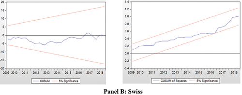
Figure 3. Plots of cumulative sum of recursive residuals (CUSUM) and cumulative sum of squares of recursive residuals (CUSUMSQ).Panel A: China Panel B: Swiss

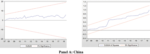
Figure 3. (Continued.)

Figure 2 demonstrates that depreciation occurs at time zero; instead of spending on domestic products, people still choose imported products because exports do not sufficiently increase, the balance of trade worsens immediately after the depreciation. After that, when import and export elasticities increased, the trade balance eventually improved. On the other hand, the supply for domestic substitutes is limited after the domestic currency devaluation. Likewise, the foreign market is similar to adjusting their buying behavior. After a short while, due to the competitive price, the volume of exports may start rising in the foreign market. As a result, the trade balance begins to be improved. This results in a “J-like” pattern in the time route of the trade balance, giving rise to the name “J-curve effect,” as shown in Figure 2.

2.2. Empirical review

Although the economic theories suggest a positive consequence for falling exchange rates on trade balance and economic growth, the results of empirical studies have been inconclusive. The empirical evidence remained mixed, with varying findings within countries and from country to country. Many researchers such as Tihomir (2004), Harvey (2005), Narayan and Narayan (2004), Thom (2017), Ongan et al. (2018a), and Bahmani-Oskooee and Jehanzeb (2009), among others, have found evidence to support the J-curve phenomenon. For instance, Bahmani-Oskooee and Cheema (2009) used disaggregated bilateral data from Pakistan’s 13 largest trading partners, which accounted for roughly 70% of total trade in 2003, to test the short-run and long-run effects of real depreciation of the Pakistani rupee. Using the Bound testing approach and Johansen’s co-integration approach, the study found evidence of the J-curve in almost half of the trading partners in the sample. Also, Tihomir (2004) finds out evidence of the J-curve effect in Croatia using a reduced form model. Hanafiah (2005) indicates evidence supporting the J-curve between Malaysia and Singapore and between Malaysia and France in the bilateral trade between Malaysia and 14 trading partners. A recent study by Ongan et al. (2018a) on the J-curve hypothesis between the United States and her major trading partners found evidence in support of the J-curve for the USA with 8 of her trading partners out of the 12 major partners covered in the study. Similarly, the study of Ahmad et al. (2021) on Pakistan also confirmed the J-curve hypothesis in Pakistan.

In contrast, several other studies also established no evidence supporting the J-curve phenomenon. For instance, Bahmani-Oskooee et al. (2006) tested the bilateral relationship between China and 13 trading partners by ARDL model in the period of 1983Q1 to 2002Q2. The results indicate that the J-curve effect and Yuan devaluation do not improve the trade balance in both the short and long run. Similarly, Ferda (2007) tested the existence of the J-curve phenomenon in the case of Turkey with her thirteen trading partners using aggregate data. This paper was carried out by bound testing approach, error correction model, and stability tests. The study shows that there is no existence of the J-curve effect in any of Turkey’s bilateral trade balance. Also, Ardalani and Bahmani-Oskooee (2007), using industrial level data, found no evidence for a J-curve, although the long-run effect of RER depreciation on the trade balance was established.

Moreover, numerous extant research has put the J-curve phenomenon to the test in a variety of developed and developing nations. African countries, however, have received little attention in this regard. Among the notable studies in Africa are Bahmani-Oskooee and Gelan (2012), Ziramba and Chifamba (2014), and Rawlins (2011), Adeniyi et al. (2011), Chiloane et al. (2014), Musila (2002), and Riti (2012). For example, Bahmani-Oskooee and Gelan (2012) used quarterly trade data of nine African countries. and bounds testing approach to co-integration and error-correction modeling to test the J-curve hypothesis. The study results couldn’t support the J-Curve for nine African countries, namely, Tanzania, Egypt, Mauritius, Kenya, Nigeria, Sierra Leone, Morocco, South Africa, and Burundi. Similarly, using aggregate trade data from 1975 to 2011, Ziramba and Chifamba (2014) examined the behavior of South Africa’s trade balance following a depreciation of the real effective exchange rate. Their empirical findings found no proof for the J-curve phenomenon in the sample.

As per the available information, the existing empirical studies on the J-curve phenomenon in the case of Ghana are very limited. Akosah and Omane-Adjepong (2017), Anning et al. (2015), Agbola (2005), Adeniyi et al. (2011), and Bhattarai and Armah (2005) are among the recent notable studies on Ghana. However, the empirical findings are mixed. For instance, Bhattarai and Armah (2005) and Akosah and Omane-Adjepong (2017) found empirical proof affirming the existence of the J-curve theory in Ghana. In contrast, Adeniyi et al. (2011) found no empirical proof of J-curve for Ghana. Therefore, this current study will throw more light on the nexus by utilizing a more robust model with a relatively large sample size to overcome the small sample size biases, a common problem amidst other issues associated with these studies in Ghana.

3. Research methodology

This section presents the main methodological strategy used in this study. This includes the variables used in the study, how the variables were calculated, the data used, and the sources of the data.

3.1. Data sources and measurement of study variables

The study relies entirely on quarterly time series data for the period of Q1-1995 to Q4-2018. The Trade Balance variable $\left(TBj,t\right)$ is calculated from the ratio of value Ghana’s Imports (IM) from partner j over her value Exports (EM) to partner j (IM/EX). The data of both exports, imports of goods, and services of Ghana with her two trading partners are obtained from International Financial Statistics (IFS). Real gross domestic product is used to measure the real income level of Ghana collected from Ghana Statistical Service $\left(Yt,t\right)$. As such, Real gross domestic product is used to measure the real income level of China and Swiss collected from International Financial Statistics $\left(Yt,t\right)$. According to Ellis (2001), the real exchange rate $\left(RERj,t\right)$ is defined as the product of $NER$ and $\left(CPI\left(j\right)\right)/\left(CPI\left(t\right)\right)$. This is expressed mathematically as $RERj,t=NER.\left(CPI{}_{(j)}\right)/\left(CPI{}_{(t)}\right)$ 1. NER is the nominal exchange rate, average-period nominal exchange rate, Ghana cedis against USD, and consumer price index $\left(CPI\right)\left(2010=100\right)$ collected from IFS.

3.2. The empirical model and approach

The trade balance model used in this study was based on the work of Bahmani-Oskooee and Fariditavana (2016) which is expressed below as;

(2) $lnTBj,t=\alpha 0+\alpha 1lnYt,t+\alpha 2lnYj,t+\alpha 3lnRERj,t+\mu 4$(2)

In the equation above, the ratio of Ghana’s nominal exports from trading partner $j$ over her nominal imports to the same country, which is presented by $T{B}_{j,t}$ (the trade balance). Y_t,t and ln $Y_{j,t}$ is the real income of Ghana and country $j$, respectively. $RE{R}_{j,t}$ is defined as the real bilateral exchange rate between Ghana cedis and country $j$‘s currency. Since an increase in domestic (Ghana) income is due to an increase in the production of import-substitute goods, I expect an estimate of $\alpha 1$ to be negative. By the same token, a positive or negative estimate of $\alpha 2$ is expected if growth in partner’s income boosts Ghana exports due to an increase in the production of import-substitute goods in the other countries. Finally, the real bilateral exchange rate between Ghana cedis and country $j$‘s currency $\left(RER\right)$ is defined in a way that the decline reflects a real devaluation of the Ghana cedis. Hence, an estimate of $\alpha 3$ should be positive if cedis depreciation improves the trade balance with partner $j$.

According to the J-curve phenomenon concept, it is common practice to separate the short-run effects of currency depreciation on trade balance from its long-run effects. Thereby, we must modify equation (2)(2) $lnTBj,t=\alpha 0+\alpha 1lnYt,t+\alpha 2lnYj,t+\alpha 3lnRERj,t+\mu 4$(2) in an error-correction modeling format. On that account, this study followed the empirical modeling of Arthur et al. (2021) and Asiedu et al. (2021) derived from the Pesaran et al.’s (2001) Autoregressive Distributed Lag (ARDL) bounds testing approach formulated as follows:

(3) $\begin{array}{rl}& \mathrm{\Delta }lnTBj,t=b0+\sum _{(i=1)}^m{b}_{1i}\mathrm{\Delta }lnTBj,t-i+\sum _{(i=0)}^m{b}_{2i}\mathrm{\Delta }lnYt,t-i+\sum _{(i=0)}^m{b}_{3i}\mathrm{\Delta }lnYj,t-i+\sum _{(i=0)}^m{b}_{4i}\mathrm{\Delta }lnRERj,t-i\\ & +b_{5}lnTBj,t-1+break{b}_{6}lnYt,t-1+b_{7}lnYj,t-1+b_{8}lnRERj,t-1+\nu t\end{array}$(3)

Where $t=year$, $m=lag$ length (which are selected on the basis of the Akaike Information Criterion), $\mathrm{\Delta }$ refers to the first difference operator, $\nu$ denotes the random disturbance term.

According to Pesaran et al. (2001), there are three outstanding advantages of the ARDL method compared to other single procedures. Firstly, there is no need to pre-testing for unit roots if the variables involved are purely I(0), purely I(1), or fractionally integrated. Secondly, endogenous problems and the inability to test hypotheses in long-term estimated coefficients identified to the Engle and Granger (1987) method were avoided. Thirdly, the short and long-run parameters of the mentioned model are estimated simultaneously. Lastly, the small sample properties belonging to the bounds testing approach are preferred to that of multivariate co-integration.

3.3. Estimation procedure

To begin, the order of integration of the variables in the model is determined using Augmented Dickey-Fuller (ADF). To determine the parameters for the ADF tests, use the equation below.

(4) $Y_t={\beta }_0+{\beta }_{1}t+{\beta }_2{Y}_{(t-1)}+\sum _{(i=1)}^k\phi Y_{(t-1)}+{\epsilon }_t$(4)

Where $\mathrm{\Delta }$ signifies the difference operator; $Y_{\begin{array}{c}t\\ \end{array}}$ implies variable $Y$ at time $t;{\beta }_0{\beta }_1{\beta }_2$ and $\phi$ are parameters to be calculated, $k$ denotes the augmented number of lags and $p_t$ the white noise term. Given equation three above, the consequent hypothesis is then tested for: $H_0$: p = 1 ($Y_{\begin{array}{c}t\\ \end{array}}$ is non- stationary) $H_1$: p < 1 ($Y_{\begin{array}{c}t\\ \end{array}}$ is stationary)

Following the variable stationary tests, the ARDL model is subjected to the bound test in order to begin the long-term relationship between the lagged variables for cutoff significance using the F test in the first stage. This is followed by an examination of the variables’ short- and long-term relationships using the direct ARDL model, as shown in Equation 3(3) $\begin{array}{rl}& \mathrm{\Delta }lnTBj,t=b0+\sum _{(i=1)}^m{b}_{1i}\mathrm{\Delta }lnTBj,t-i+\sum _{(i=0)}^m{b}_{2i}\mathrm{\Delta }lnYt,t-i+\sum _{(i=0)}^m{b}_{3i}\mathrm{\Delta }lnYj,t-i+\sum _{(i=0)}^m{b}_{4i}\mathrm{\Delta }lnRERj,t-i\\ & +b_{5}lnTBj,t-1+break{b}_{6}lnYt,t-1+b_{7}lnYj,t-1+b_{8}lnRERj,t-1+\nu t\end{array}$(3) . The presence of co-integration is then validated by measuring the F-statistic value for the combined lagged levels of the variables and comparing it to the values of the critical bounds. This is accomplished by analyzing the subsequent bound test hypothesis:

$H_0=b_{1i}=b_{2i}=b_{3i}=0$ (No co-integration)$\begin{array}{rl}& H_1=b_{1i}=b_{2i}=b_{3i}\ne 0\\ & \end{array}$ (co-integrated)

The calculated F statistical value is compared to the critical values of Pesaran et al. (2001). If the estimated F statistic number is less than the lower critical limit number, we accept the null hypothesis and conclude that there is no co-integration between the variables. If, on the other hand, the calculated F statistic exceeds the upper critical limit, we reject the null hypothesis and declare that there is a long-term equilibrium relationship between the variables under consideration. However, if the calculated F statistic value is between the lower and upper critical limit values, the co-integration test result is inconclusive. The presence of co-integration indicates that the series has a long-term relationship. If co-integration is discovered between the variables, the long-run series relationship and short-run or error correction model $\left(ECM\right)$ can be estimated separately as follows:

3.3.1. Long-run relationship estimate

(5) $lnTBj,t=\alpha 0+\alpha 1lnYt,t+\alpha 2lnYj,t+\alpha 3lnRERj,t+\mu 4$(5)

3.3.2. Error correction model estimate

(6) $lnTBt=b0+\sum _{(i=1)}^m{b}_{1i}lnTBt-i+\sum _{(i=0)}^m{b}_{2i}lnTBt,t-i+\sum _{(i=0)}^m{b}_{3i}lnTBj,t-i+\sum _{(i=0)}^m{b}_{4i}lnRERt-i+\lambda ECMt-1+\mu t$(6)

Where $\lambda$ is the speed of adjustment parameter; $\left(ECM\right)$ or error term is the residuals that are archived by estimated normalized coefficient in model of equation (5)(5) $lnTBj,t=\alpha 0+\alpha 1lnYt,t+\alpha 2lnYj,t+\alpha 3lnRERj,t+\mu 4$(5) . $\begin{array}{rl}& b_{1i},b_{2i},b_{3i}\\ & \end{array}$ are the short-run dynamic coefficient of the model’s adjustment long-run equilibrium. The expectation for the value of α₁ is negative, the positive value of $\alpha 2$ is anticipated, and the estimate of $\alpha 3$ is expected to be positive. Bahmani-Oskooee and Jehanzeb (2009) stated that a significant negative coefficient, $ECMt-1$, supports co-integration and the size of the coefficient quantifies the speed of convergence towards equilibrium.

Lastly, the validity and reliability of the parameters of the results obtained are proven using a variety of diagnostic tests such as Ramsey RESET, Hetreoscedacity, serial correlation, the cumulative sum of recursive residuals (CUSUM), and cumulative sum of the square of the recursive residuals (CUSUMSQ) statistics.

4. Results and discussion

4.1. Unit root test

The stationary characteristics of the variables were verified with the Augmented Dickey-Fuller (ADF) test to ensure that the precondition for estimating an ARDL model is met. The results in Table 1 indicate the non-existence of the I(2) variable in our study. It is also evident from the results that in the exception of the real exchange rate between Ghana and China (lnRER_GH-CN), which is stationary upon first difference, all the other variables are stationary at level.

Table 1. Test for unit root

Variables	ADF Test		I(n)
	Level	1st-diff
lnTBGH-CN	−0.450		I(0)
lnTBGH-SW	−2.311*		I(0)
lnRERGH-CN	−1.075	−1.688*	I(1)
lnRERGH-SW	−3.154*		I(0)
lnYGH	−1.859		I(0)
LnYCN	−2.848*		I(0)
LnYSW	−2.594		I(0)

Note: The statistical significance is denoted as *, **, and *** for 10%, 5%, and 1% respectively. Additionally, ADF test is Augmented Dickey–Fuller test, Level defines level form, and the first difference form is defined as 1st-diff. GH is Ghana, SW is Switzerland and CN is China.

4.2. Co-integration test

The ARDL bound test or co-integration test was calculated once the precondition for estimating an ARDL model was met. This was done to see if there were any long-term relationships between the core variables. Table 2 contains the results of the ARDL bound test or co-integration.

Table 2. Bounds test

Trading partner	Dependent variables ΔlnTBt	F-statistics	Critical Value Bonds of the F-statistics						Outcome
			95%		97.5%		99%
			I(0)	I(1)	I(0)	I(1)	I(0)	I(1)
China	ARDL (4, 5, 3, 4)	8.039	2.79	3.67	3.15	4.08	3.65	4.66	Co-integration
Swiss	ARDL (1, 1, 3, 3)	9.024							Co-integration

The optimal lag order for the ARDL model is selected by using the Akaike information criterion (AIC). The results indicate that the F-statistic for the joint significance of the parameters of the lagged level variables exceeds the Pesaran et al. (2001) small sample upper bound critical values. Thus, there is evidence of co-integration between the variables at 1 percent for both China and Swiss. Hence, the null hypothesis is rejected, which is found that there is a long-run relationship in bilateral trade balance with domestic income, foreign income, and real effective exchange rate in the case of two countries. Given the existence of co-integration or a long-term relationship between the variables, the study proceeds with the estimation of both the long-term and short-term relationship (Vector Error Correction Model).

4.3. Regression results

The short- and long-run results of the ARDL model are provided in Table 3 with Panel A and Panel B for China and Swiss, respectively. It is worth noting that the lagged error correction term in Table 3, $ECMt-1$, is negative and significant in both cases of China and Swiss. As posited by, Bahmani-Oskooee and Jehanzeb (2009)—have shown that the significant lagged error correction term is a more efficient way of establishing co-integration. Hence, by this criterion, it could be confirmed that all variables in equation (3)(3) $\begin{array}{rl}& \mathrm{\Delta }lnTBj,t=b0+\sum _{(i=1)}^m{b}_{1i}\mathrm{\Delta }lnTBj,t-i+\sum _{(i=0)}^m{b}_{2i}\mathrm{\Delta }lnYt,t-i+\sum _{(i=0)}^m{b}_{3i}\mathrm{\Delta }lnYj,t-i+\sum _{(i=0)}^m{b}_{4i}\mathrm{\Delta }lnRERj,t-i\\ & +b_{5}lnTBj,t-1+break{b}_{6}lnYt,t-1+b_{7}lnYj,t-1+b_{8}lnRERj,t-1+\nu t\end{array}$(3) have long-run relationship for each country. The negative coefficients followed by positive ones in the short-run coefficient estimates will support the J-Curve phenomenon. From Table 3, the results indicate some evidence of a J-Curve for China but not in Swiss

Table 3. ARDL model results

Panel A. China
Variable	Coefficient	Std. Error	t-Statistic	Prob.
Dependent variable: ΔlnTBt
Long-run elasticities
C	−40.282***	7.972	−5.052	0.000
lnRER(−1)	3.235***	0.647	4.999	0.000
lnYGH(−1)	−0.037	0.093	−0.402	0.689
lnYCN(−1)	1.045***	0.267	3.903	0.000
Short-run elasticities
C	0.172***	0.063	2.710	0.010
ΔlnTB(−1)	−0.364***	0.145	−2.497	0.017
ΔlnTB(−2)	0.195*	0.134	1.450	0.155
ΔlnTB(−3)	0.311**	0.166	1.867	0.070
ΔlnTB(−4)	−0.357**	0.160	−2.229	0.032
ΔlnRER	−1.338	1.090	−1.227	0.227
ΔlnRER(−1)	−0.306	1.306	−0.234	0.815
ΔlnRER(−2)	−1.052	1.353	−0.777	0.442
ΔlnRER(−3)	−0.360	1.301	0.276	0.783
ΔlnRER(−4)	0.469	1.348	0.348	0.729
ΔlnRER(−5)	2.762**	1.212	2.277	0.028
ΔlnYGH	0.348***	0.114	3.054	0.004
ΔlnYGH(−1)	0.391***	0.115	3.406	0.001
ΔlnYGH(−2)	0.332***	0.108	3.054	0.004
ΔlnYGH(−3)	0.351***	0.102	3.423	0.001
ΔlnYCN	1.460	1.335	1.092	0.281
ΔlnYCN(−1)	−2.103***	0.785	−2.677	0.011
ΔlnYCN(−2)	−2.573***	0.785	−3.275	0.002
ΔlnYCN(−3)	−2.137***	0.767	−2.783	0.008
ΔlnYCN(−4)	−3.623**	1.770	−2.046	0.048
ECM(−1)	−0.142**	0.079	−1.797	0.080
Panel B. Swiss
Variable	Coefficient	Std. Error	t-Statistic	Prob.
Long-run elasticities
C	−26.574***	7.031	−3.779	0.000
lnRER(−1)	1.594***	0.285	5.589	0.000
lnYGH(−1)	0.014	0.055	0.271	0.787
lnYSW(−1)	1.498***	0.592	2.529	0.014
Dependent variable: ΔlnTBt
Short-run elasticities
C	−0.031*	0.023	−1.363	0.179
ΔlnTB(−1)	−0.065	0.151	−0.434	0.665
ΔlnRER	0.689	0.854	0.806	0.424
ΔlnRER(−1)	−0.674	0.872	−0.773	0.443
ΔlnYGH	0.042	0.086	0.488	0.627
ΔlnYGH(−1)	0.104	0.084	1.234	0.223
ΔlnYGH(−2)	0.025	0.081	0.315	0.753
ΔlnYGH(−3)	0.076	0.080	0.950	0.346
ΔlnYSW	−0.637	0.975	−0.652	0.517
ΔlnYSW(−1)	−3.031	2.442	−1.240	0.221
ΔlnYSW(−2)	5.324**	2.483	2.144	0.037
ΔlnYSW(−3)	3.592*	2.523	1.423	0.161
ECM(−1)	−0.194**	0.086	−2.232	0.030

Note: ***, **, * represents 1%, 5% & 10% significance level, respectively

From the results of China in Panel A of Table 3, there is evidence for the J-curve phenomenon in the bilateral trade between Ghana and China. Following the expectations, the results show that Ghana’s trade balance deteriorates in the short run. Then it improves after four quarters (one year). In the short-run, exchange rate change has an immediate negative effect on Ghana’s exports to imports trade ratio. The short-run results indicate that a 1 percent increase in the real exchange rate of Ghana cedis against the Chinese Yuan (that is, depreciation of the Ghana cedis) is followed by an immediate 0.67 percent increase in Ghana’s trade balance with China. A 1 lagged real exchange rate is found to have a significant negative impact on trade, decreasing Ghana’s trade balance by 0.89 percent. After that, it shows the positive effect on Ghana’s trade balance at 2 and 3 lagged. Generally, the response of Ghana’s exports to imports trade ratio to the change in the real exchange rate is not surprising and may be attributed to the factor that China is the largest importer of Ghana, especially the automobiles or kinds of material for local industries. As a result, along with the Ghana cedis devaluation, the amount of money to buy materials for manufacturing would become more expensive. In contrast, the exported commodities from Ghana would become cheaper at the same time, but foreign customers still need the time to adjust their shopping behavior. That leads to the immediate decrease in the trade balance in the short run, followed by the expectation of an increase in the long run. The long-run results show that a rise in the real exchange rate change (or a real depreciation) of the Ghana cedis has a significantly anticipated positive effect on Ghana’s trade balance with China. In the long-run, 1 percent depreciation of the real Ghana cedis against the Yuan leads to a 3.24 percent increase in trade balance at 1 percent significance. The finding here is contrary to the arguments made by Adeniyi et al. (2011), who found no empirical proof of J-curve for Ghana.

Meanwhile, the short-run impact of China and Ghana’s real GDP also explained the slow adjustment of consumers’ behavior in China and Ghana to the change in prices. In the case of Ghana’s income effect, an increase in its real gross domestic product has the expected effect of lowering its bilateral trade balance with China as Ghanaian output may be switched to meet an increase in its domestic demand.

However, the positive impact occurs immediately and also with the following lags. Besides, in the case of China’s income, an increase in China’s real GDP has a positive impact on Ghana’s export-import trade ratio after one quarter, decreasing it by 2.1 percent for every 1 percent increase in the China real GDP. Following that, the impact of the lagged values of China’s real GDP for up to four periods is also negative. This suggests that the price of goods exported by China in Ghana was more competitive than domestic products. Most Chinese products may generally be categorized as “inferior goods,” though the demand would decrease when Ghana’s real income increased. Besides, Ghana had a lot of policies to push the demand for domestic commodities in the domestic market. Moreover, although the growing share of Gold in oth semi-manufactured forms by Ghana in recent years, most of Ghana’s exports to China may basically face small demand with increased China income level rises.

With respect to the long-run results on real income, Ghana’s income has a significant negative coefficient as expected. Hence, imports from China decline as Ghana’s economy grows. As shown in the setup of this model, this may be because of the substitution effect, import less from these partners as Ghana produces domestic substitutes. As estimated, China’s income is expected to be positively correlated with Ghana’s trade balance since China’s economic growth will promote Ghana’s exports.

Overall, it may be concluded from these findings that, in the long-term, Ghana’s exports to imports ratio is most responsive to a change in China’s income and the real exchange rate than to Ghana’s domestic income change. Following the negative effect in the short term, the positive effect in the long term indicates the J-curve phenomenon in the case of China. The results confirm that the devaluation of the Ghana cedis, in this case, might bring benefit for Ghana trade balance.

Panel B of Table 4, On the other hand, reports the results of Swiss. It is worth noting from the results that the J-curve is not found in the relationship between Ghana and Swiss unlike the inelastic response of trade ratio to a change in the cedis’ exchange rate in the short-run, results for real exchange rate has a positive effect immediately on trade balance between Ghana and Swiss at 0.69 percent, followed by negative effect at 1-quarter lag at −0.67 percent. However, the long-run results indicate that a depreciation of the real exchange rate change of the Ghana cedis has a significant and positive effect on the bilateral trade balance. In the long run, Ghana’s trade balance registers an elastic response measured at a 1.594 percent increase to a 1 percent depreciation of the real Ghana cedis against the Swiss franc. The time lag is an important factor to observe clearly whether there is a sign of a J-curve pattern or not. Himarios (1985) pointed out that the lagged values of exchange rates played a role. It is clearly seen from the results that the negative impact on trade balance just lasted in 1 quarter, so the evidence for J-curve shape, in this case, is not strong enough to conclude that there is the existence of the J-curve effect.

Table 4. Diagnostic tests results

Test	China	Swiss
Serial Correlation LM Test	0.6420	0.9160
Ramsey RESET	0.9621	0.3448
CUSUM	ARDL model is stable	ARDL model is stable
CUSUMSQ	ARDL model is stable	ARDL model is stable

The inelastic response of Ghana’s exports to imports trade ratio to the change in the real exchange rate may be caused by lags in the renegotiation of international trade contracts. Related to the impact of Ghana and the Swiss’ real income, the results are quite the same with the case of China. Ghana’s real income has a positive effect on the trade balance, but a negative effect is found for the Swiss’s real income. The negative impact occurs immediately at −0.64 percent and a 1-year lag at −3.03 percent. However, the impact of the lagged values of Swiss’ real GDP for up to two periods is positive and significant. In the case of Ghana’s income, a rise in Ghana’s real GDP also has an immediate positive impact on China’s export-import trade ratio by 0.04 percent, followed by 0.1 percent in a 1-year lag for every 1 percent increase in the Ghana real GDP.

Despite the J-curve phenomenon not being found in this case, there is evidence for the improvement of the trade balance between Ghana and Swiss by changes in the real exchange rate. This result may be attributed to the increasing Ghanaian output and exports of more cleavage products coupled with higher import content and intra-company trade (particularly by American companies) as well as the ability of Ghana’s exporting firms to deal with exchange rate changes. Also, with respect to the long-run impact of real GDP, a 1 percent increase in Swiss real GDP increased Ghana’s trade balance to rise by 1.5 percent at 1 percent significance. This suggests that most of Ghana’s exports to Swiss, which are cleavage products, may generally be considered as “essential goods” with higher demand when the US income level rises. On the other hand, an increase in Ghana’s real GDP has a small positive effect at 0.01 percent on the trade balance.

In general, it may be concluded from these findings that, in the long-term, Ghana’s exports to imports ratio is most responsive to a change in the trading partner’s income and the real exchange rate change than to Ghana’s domestic income change.

4.4. Post estimation diagnostic results

This study applies a variety of different diagnostic tests to the model to evaluate the reliability of obtained coefficients and the validity of the model. The results are reported in Table 4. The diagnostic test results show the absence of serial correlation as well as heteroscedasticity for both China and Swiss. Moreover, Figure 3 (Panel A and B) also displays CUSUM and CUSUMSQ statistics plots within the critical bounds at a 5 percent significance level. Panel A and Panel B indicate the results for China and Swiss, respectively.

From Table 4, the Breusch‐Godfrey serial correlation LM test with one degree of freedom of distribution shows both countries pass the test, implying autocorrelation‐free residuals in this study’s models, at a 5 percent level of significance. Likewise, no result for failing Ramsey’s RESET test, at a 5 percent level of significance, indicating that models are correctly specified in general. The stability of the coefficient estimates over time is examined by using the cumulative sum of recursive residuals (CUSUM) test and the cumulative sum of squares of recursive residuals (CUSUM of Squares). The CUSUM and CUSUMSQ test results for both the case of China and Swiss stay inside the boundaries. This indicates that the model of bilateral trade between Ghana and these major trading partners is stable over time.

5. Conclusion and policy implications

Various empirical studies investigate the J-Curve phenomenon by employing a trade balance model. However, developing countries have not received much attention in this regard. This paper examines the J-Curve phenomenon of a developing country in the case of Ghana and its major trade partners: Switzerland and China. This study exerts quarterly bilateral data from Q1-1995 to Q4-2018 to investigate the nexus of currency depreciation and bilateral trade balance in short in the short and the long run. Using the ARDL co-integration technique, the following key findings were established:

Firstly, in the short run, the real depreciation of Ghana cedis improves Ghana’s trade balance with China and the Swiss after worsening the trade balance. Secondly, in the long run, the Ghana trade balance is improved from a real depreciation of cedis which formed 3.235 percent and 1.594 percent of Ghana’s total trade share with China and Swiss, respectively. Thirdly, the estimates in this paper demonstrate that there is evidence of the J-Curve phenomenon only in the cases of China, not for Swiss, even though both China and Swiss are the largest and the second-largest trading partners respectively of Ghana. Fourthly, the results suggest that the trade balance between Ghana and China deteriorated for one year before it improved. Moreover, the examination of these issues is appropriate for the real situation in the present. Furthermore, the real income of trading partners had a positive and significant effect in the long run, similar to the expected sign according to the model, meaning that an increase in the real income of partners is found to have an important role in determining imports from Ghana. However, there is no significant effect on Ghana’s real income on the trade balance. Finally, the CUSUM and CUSUMSQ stability tests and other diagnostics tests results for the model show that the estimated relationships have been stable and reliable over the last 24 years.

Consequently, the empirical results reflect the following key policy recommendations. First, the J-curve analysis shows that a devaluation of the cedis would help to improve the trade balance in the long run. The results imply that the exchange rate policy is still a significant tool to manage Ghana’s trade deficit with two main trading partners, China and Swiss. Therefore, it is recommended that the government ensure a competitive exchange rate policy to boost its trade balance. Secondly, the study recommends diversification of the country’s exports to improve the balance of trade. As such, value additions and non-traditional export industries, in particular, should be given special attention. Lastly, it is also vital for the monetary authority to maintain macroeconomic stability (inflation) to foster the private sector’s growth. This necessitates the implementation of suitable and well-coordinated monetary and fiscal policies that result in low and stable inflation and stable foreign exchange rates.

5.1. Limitations and recommendations for future research

Our study, like any other, has some limitations that may open the door for future related lines of research. First, though the current study outcome offers an aggregate insight on the nexus of bilateral exchange rate and trade balance of Ghana, future research should look at the impact of bilateral exchange rates on the trade balances at the industry level. Analyzing the connection between bilateral exchange rates and trade balances at the industry level will also allow for a comprehensive evaluation of the industry’s contribution to the trade balance correction. In addition, identifying the scope and effects of this industry relationship can aid policymakers in developing more effective strategies and policies to boost and manage the trade balance. Lastly, although the study examined the effects of exchange rate movement on the balance of trade, other factors such as policy uncertainty and pandemics may influence the nexus, which the study couldn’t capture. As such, we recommend that future studies consider these variables’ role in the models.

Disclosure statement

No potential conflict of interest was reported by the author(s).

Additional information

Funding

The authors received no direct funding for this research.

Notes on contributors

Benedict Arthur

Benedict Arthur is a Researcher at the School of Finance, Zhongnan University of Economics and Law in China. His current research interests span across International Finance, Monetary Economics, Sustainability, Corporate Governance, and Finance.

Millicent Selase Afenya

Millicent Selase Afenya is a Ph.D. accounting student at Zhongnan University of Economics and Law. Her main research interests lie in the area of Auditing and Corporate Governance.

Michael Asiedu

Michael Asiedu is a Ph.D. student in Finance at Zhongnan University of Economics and Law in Wuhan - China. His research interests include securities analysis, asset valuation and pricing, financial innovation and inclusion, monetary policy, and growth theories.

Rebecca Aduku

Rebecca Aduku is a master’s student at Zhongnan University of Economics and Law in China. She majors in International Business, and her current interest lies in international trade policies and E-commerce.